Dynamic Reconfiguration of Active Distribution Network Based on Improved Equilibrium Optimizer

Abstract

To better address the reconfiguration problem of distribution networks with distributed generation (DG), a dynamic reconfiguration model is developed that accounts for the time-varying characteristics of both load demand and DG output. First, an enhanced fuzzy C-means clustering method is proposed for load period partitioning, which integrates spatiotemporal load features and optimal network structure similarity to improve clustering accuracy. Second, an adaptive ordered loop-based feasibility judgment model is developed to filter infeasible and low-quality solutions based on operational constraints. Third, an improved Equilibrium Optimizer (IEO), integrating Tent chaotic initialization, elite sorting, and mutation-crossover strategies, is proposed for multi-objective optimization. The proposed framework is validated on IEEE 33- and 69-bus systems. In the IEEE 33-bus system, it achieves a 44.8% reduction in power losses and a 35.9% improvement in voltage deviation. In the IEEE 69-bus system, power loss is reduced by 40.1%, and voltage deviation by 40.5%, demonstrating the proposed method’s robustness, adaptability, and effectiveness across systems of varying scales.

1. Introduction

The distribution network comprises a large number of normally closed and open switches. The primary objective of network reconfiguration is to alter the network topology by adjusting the status of line switches, thereby achieving load balancing across feeders, mitigating overloads, reducing power losses, and restoring faults to enhance the system’s power supply capability [1]. In recent years, the increasing integration of distributed generation (DG), such as wind and photovoltaic energy, into power systems—due to their environmental benefits and renewability—has made active distribution network reconfiguration a prominent research focus. However, the inherently intermittent and fluctuating output of DGs can lead to complications such as bidirectional power flow, voltage violations, and line overloading, which pose challenges to grid reliability. Against this backdrop, distribution network reconfiguration has gained attention as a viable solution to improve operational efficiency and system stability.

Reconfiguration approaches are generally classified into static and dynamic methods. Static reconfiguration adjusts the network topology based on the load status at a single time point, often overlooking temporal variations in load, thus failing to meet the requirements of real-time operation. In contrast, dynamic reconfiguration adapts the network structure in response to real-time system changes, offering greater practicality. Currently, a key research challenge lies in how to segment load periods and decompose dynamic reconfiguration into a series of interrelated static reconfiguration tasks under fluctuating loads and DG outputs. Behbahani et al. [2] provided a comprehensive review of static and dynamic distribution network reconfiguration methods, highlighting the potential of dynamic reconfiguration in modern smart grids and classifying existing approaches into five methodological categories: classical methods, heuristic methods, metaheuristic methods, hybrid methods, and methods based on machine learning. Furthermore, Behbahani et al. [2] noted that while machine learning methods are suitable for dynamic reconfiguration due to their real-time adaptability, metaheuristic algorithms remain highly competitive in dynamic reconfiguration problems, owing to their flexibility, objective versatility, and proven optimization accuracy.

The reconfiguration problem in distribution networks is inherently a complex, large-scale, nonlinear, and combinatorial optimization challenge [3]. In recent years, a variety of intelligent optimization algorithms—such as Genetic Algorithms [4,5], Particle Swarm Optimization [4,6,7], Grey Wolf Optimization [8], and Cuckoo Search Algorithm [9]—has been widely adopted for this task. Furthermore, Maurya et al. [10] introduced the Electric Eel Foraging Optimization algorithm for joint DG placement and network reconfiguration, achieving over 90% improvement in power loss and voltage deviation in typical test systems. Musaruddin et al. [11] employed a Selective Particle Swarm Optimization algorithm for practical DN reconfiguration, achieving reductions in power loss and improvements in voltage profile under various load scenarios. Cikan and Cikan [12] applied the Slime Mold Algorithm to reconfigure a 123-bus unbalanced distribution system, effectively reducing power loss and minimizing current and voltage unbalance indices. Anteneh et al. [13] employed a modified shark smell optimization algorithm for DN reconfiguration in a real Ethiopian system, achieving simultaneous improvements in reliability indices, voltage profile, and power loss reduction. Iftikhar and Imran [14] proposed improved hybrid optimization schemes combining GA and TLBO for joint DER integration and network reconfiguration, achieving significant improvements in power loss and voltage performance across standard test systems. Manikanta et al. [15] employed an Adaptive Quantum-inspired Evolutionary Algorithm to optimize network reconfiguration with DG and capacitor allocation, achieving simultaneous power loss reduction and economic benefit maximization. Rahmati and Taherinasab [16] utilized the dragonfly optimization algorithm for distribution network reconfiguration, demonstrating superior energy loss reduction through coordinated control of tap transformers and DG power factors. Tao et al. [17] developed a dynamic simulated annealing particle swarm optimization (DSAPSO) algorithm for distribution network reconfiguration with DGs, effectively improving convergence speed and reducing power losses while enhancing voltage stability. Fathi et al. [18] proposed an improved salp swarm algorithm integrating differential evolution operators for simultaneous DG allocation and network reconfiguration, achieving notable reductions in power loss cost and reliability improvement expenses. Notably, the Equilibrium Optimizer (EO), introduced by Afshin Faramarzi et al. [19] in 2020, is inspired by the principle of mass balance in physics. Cikan and Kekezoglu [20] conducted a comprehensive statistical comparison of metaheuristic algorithms for distribution network reconfiguration and demonstrated that the Equilibrium Optimizer consistently outperformed ten other methods in terms of loss reduction, voltage improvement, and reliability enhancement across multiple test systems. Shaheen et al. [21] developed an improved equilibrium optimization algorithm (IEOA) incorporating a recycling strategy to enhance global search capability for the joint problem of network reconfiguration and distributed generation allocation. The method was validated on IEEE 33-bus, 69-bus, and 137-bus systems under multiple load levels, demonstrating significant reductions in active power losses and improvements in voltage profiles. Comparative analysis with other metaheuristics—including harmony search, genetic algorithm, and firefly algorithm—confirmed the superior robustness and effectiveness of the proposed approach in handling complex multi-objective optimization problems. Despite these successes, several limitations remain. Due to the stochastic nature of intelligent algorithms, they are prone to local optima. Furthermore, their randomness often results in the generation of a large number of infeasible or suboptimal solutions during the search process, expanding the solution space unnecessarily and increasing computational cost [22,23]. A particularly critical requirement is ensuring that generated solutions adhere to the radial topology constraint of distribution networks. Thus, improving algorithm performance and reducing infeasibility remain pressing challenges. Recent studies have attempted to address these issues using advanced strategies such as multi-objective frameworks, scenario-based uncertainty modeling, and hybrid metaheuristics [24,25,26,27,28,29]. However, most still lack dynamic adaptability and robust feasibility assurance mechanisms, particularly under time-varying load and DG outputs—gaps that this study aims to bridge.

Therefore, the main contributions of this study are summarized as follows:

(1)

Improved load period division: A fuzzy C-means clustering method is enhanced by incorporating time-weighted load similarity and optimal network topology similarity, resulting in more accurate and stable time segmentation.

(2)

Feasibility judgment innovation: An adaptive ordered loop-based feasibility model is proposed to rigorously eliminate infeasible and low-quality solutions by enforcing power balance and topological constraints.

(3)

Enhanced optimization algorithm: An improved Equilibrium Optimizer (IEO) is developed by incorporating Tent chaotic initialization, elite non-dominated sorting, stochastic mutation, and binomial crossover, significantly enhancing convergence and global search capabilities.

(4)

Integrated reconfiguration framework: A unified dynamic reconfiguration framework is constructed by coupling the proposed clustering, feasibility evaluation, and optimization methods. The framework is validated on IEEE 33- and 69-bus systems, demonstrating superior performance in reducing power loss and improving voltage stability.

The remainder of this paper is organized as follows: Section 2 presents the proposed load period segmentation method based on the improved fuzzy C-means clustering algorithm, including the incorporation of spatiotemporal similarity and adaptive time weighting. Section 3 describes the formulation of the multi-objective optimization model. Section 4 details the construction of the feasibility judgment model based on the basic ring matrix and discusses the enhancement strategies applied to the standard Equilibrium Optimizer (EO) and presents the design of the Improved Equilibrium Optimizer (IEO). Section 5 reports the results of simulation experiments conducted on IEEE 33- and 69-bus systems, compares the performance of the proposed method with other state-of-the-art algorithms, and validates its effectiveness and robustness. Finally, Section 6 summarizes the main conclusions and outlines future research directions.

2. Load Period Partitioning Method Based on Improved Fuzzy C-Means Clustering

Considering the temporal characteristics of distributed generation and load profiles, this paper proposes an improved fuzzy C-means (FCM) clustering algorithm to effectively capture the dynamic variations in distribution network loads in response to real-time system status changes. The proposed method divides the typical load characteristics of the distribution network into representative time periods.

FCM is a clustering algorithm grounded in fuzzy set theory. In contrast to traditional hard clustering techniques such as K-means, FCM does not rigidly assign each data point to a single cluster. Instead, it employs a membership function that allows each sample to simultaneously belong to multiple clusters with varying degrees of membership. This soft partitioning approach enhances FCM’s flexibility and representational capability, particularly when handling data with ambiguous boundaries or indistinct structures, thereby making it a popular tool in load analysis.

To address the limitations of the traditional FCM algorithm—specifically its deficiencies in clustering accuracy, stability, and feature representation when applied to load period division—this study introduces an improved FCM method. The improvement lies in incorporating a comprehensive similarity measure and a time-weighted similarity matrix, enabling more precise and reliable segmentation of distribution network load curves into distinct time intervals.

2.1. Comprehensive Similarity Calculation Based on Load Characteristics and Optimal Network Structure

The higher the similarity of loads and the optimal network configurations across different time periods, the greater the likelihood that the same network topology can be applied after time periods are merged [30,31,32]. Therefore, this study jointly considers both load similarity and optimal network structure similarity to evaluate the degree of resemblance between any two time periods. By ensuring that periods with similar load patterns or identical optimal structures are assigned higher similarity scores, a clustering process based on comprehensive similarity is employed to determine the final time division scheme.

In this study, distribution network reconfiguration is performed using next-day load forecasts. The day is initially segmented evenly into T time intervals (T = 24 in this case). It is assumed that the load at each node remains constant within a single time period. The load characteristic vectors for time periods a and b are defined by Equations (1) and (2), respectively.

$$X_a=(x_{a1},x_{a2},\dots ,x_{an})$$

(1)

$$X_b=(x_{b1},x_{b2},\dots ,x_{bn})$$

(2)

where n is the number of load characteristics, x_ak represents the kth load characteristic of the time period a, x_bk represents the kth load characteristic of the time period b, and the Euclidean distance $d(X_a,X_b)$ between time periods a and b is shown in Equation (3):

$$d(X_a,X_b)=\sqrt{{\displaystyle \sum _{k=1}^n{(x_{ak}-x_{bk})}^2}}$$

(3)

In order to facilitate the representation of load similarity, the Euclidean distance is converted into a similarity index, in Equation (4):

$$S_{ab}^l={\displaystyle \frac{1}{1+d\left(X_a,X_b\right)}}$$

(4)

where $S_{ab}^l$ represents the load similarity between time periods a and b. The smaller the Euclidean distance d, the closer $S_{ab}^l$ is to one, indicating that the load characteristics are more similar. Conversely, the closer d is to zero, the greater the difference in load characteristics.

To further quantify the similarity between optimal network structures across different time periods, this study introduces a structural similarity index based on the degree of overlap among disconnected switches. Specifically, for each initial time interval, static reconfiguration of the distribution network is performed to determine the optimal topology under the prevailing load conditions. The sets of switches that must be disconnected are recorded as Q_i and Q_j, corresponding to time periods t_i and t_j, respectively.

Given the potential variation in the number of switches required to be disconnected across different time periods, directly evaluating similarity using the ratio of the intersection size to that of a single set may introduce bias. To address this issue, this study adopts the Jaccard coefficient, widely used in set similarity analysis, as the metric for defining the similarity of optimal network structures, as presented in Equation (5).

$$S_{ab}^N={\displaystyle \frac{\left|Q_i\cap Q_j\right|}{\left|Q_i\cup Q_j\right|}}$$

(5)

where $\left|Q_i\cap Q_j\right|$ represents the intersection number of switch numbers that need to be disconnected in two time periods, $\left|Q_i\cup Q_j\right|$ represents the number of its union sets. This indicator can adaptively change between 0 and 1, and when the switches that need to be disconnected in two time periods are exactly the same, $S_{ab}^N=1$; if there is no complete overlap, then $S_{ab}^N=0$. This definition not only eliminates the bias caused by an unequal number of disconnections but also has good normalization characteristics, making it easy to integrate with load similarity to construct a comprehensive similarity index in the future.

To calculate the comprehensive similarity, a weighted fusion method is used based on the comprehensive influence of load characteristics and network structure, as illustrated in Equation (6).

$$S_{ab}^{base}=\alpha S_{ab}^l+(1-\alpha )S_{ab}^N$$

(6)

To balance the influence of temporal similarity and optimal network structure similarity in the comprehensive similarity index, we introduce a weight coefficient α, whose value ranges from 0 to 1. A higher value of α increases the emphasis on temporal features, while a lower value emphasizes structural similarity. In this study, α is empirically set to 0.5 to equally reflect both aspects. This setting was selected based on empirical sensitivity analysis, which showed that it provides a robust trade-off between clustering accuracy and adaptability under varying load patterns. The final comprehensive similarity $S_{ab}^{base}$ reflects the overall similarity between any two time periods a and b, providing a basis for subsequent clustering.

The comprehensive similarity calculation method based on conforming features and optimal network architecture proposed in this article only requires static reconstruction for each initial time period, which significantly reduces the computational complexity compared to the method of partitioning and reconstructing at different time periods to minimize network loss. Compared with the clustering method based solely on load characteristics, the method proposed in this paper also considers the situation where the load differences are large but the optimal network structure is the same, which increases the possibility of applying the same network structure after merging time periods.

2.2. Time-Weighted Similarity Matrix Calculation Method

The comprehensive similarity evaluation approach proposed in this paper—based on both load characteristics and optimal network topology—only requires static reconstruction for each initial time period. This substantially reduces computational complexity compared to traditional methods that perform repeated reconstruction across all time segments to minimize network loss. Furthermore, unlike clustering techniques that rely solely on load profiles, the proposed method also accounts for cases where significant load variation exists but the resulting optimal network structures remain identical. This enhances the feasibility of applying unified network configurations across merged time periods.

Assuming the current time period is t, a time weighting factor is introduced to include the information of the previous and subsequent time periods in the calculation. The specific formula is shown in Equation (7):

$$S_{ab}^{time}=\epsilon S_{ab}^{base}+\lambda S_{a-1,b}^{base}+\gamma S_{a+1,b}^{base}$$

(7)

where $S_{ab}^{base}$ is the comprehensive similarity of the current time period, $S_{a-1,b}^{base}$ and $S_{a+1,b}^{base}$ are the similarity between the previous and subsequent time periods, $\epsilon +\lambda +\gamma =1$ and usually $\epsilon >\lambda \ge \gamma$.

In Equation (7), the temporal weight coefficients $\epsilon ,\lambda ,\gamma$ are designed to reflect the decaying importance of historical data over time. Specifically, we adopt an exponential decay scheme to assign higher weights to more recent load data. These coefficients are normalized such that $\epsilon +\lambda +\gamma =1$, ensuring consistency across different time lengths. This weighting mechanism allows the algorithm to focus more on current trends while still incorporating useful historical information.

By introducing a time-weighted similarity matrix to fuse time-series information, it is possible to smooth out abrupt load features, reduce the impact of outliers, and ensure the continuity of time period division results, thereby making the time period division results more accurate and reliable.

2.3. Improved FCM Algorithm with Adaptive Clustering and Temporal Feature Fusion

Following the computation of both comprehensive similarity between time periods and the time-weighted similarity matrix, this study employs the Fuzzy C-Means (FCM) algorithm to perform time period segmentation. As a distance-based clustering technique, FCM allows each time segment to belong to multiple clusters simultaneously, assigning higher membership values to the most representative cluster. This characteristic makes FCM particularly suitable for handling ambiguous boundaries and transitional patterns in load profiles, thereby more accurately capturing real-world fluctuations in electricity demand.

Nevertheless, the conventional FCM algorithm exhibits limitations in clustering stability and accuracy when applied to time-based load partitioning. To address these issues, this paper introduces the following enhancements to improve its overall performance.

(1)

Introducing Comprehensive Similarity as an Input Feature

The traditional FCM algorithm utilizes Euclidean distance to assess differences between samples, directly computing distances based on physical attributes such as load and voltage. However, this approach often fails to effectively capture the underlying correlations between features—particularly in scenarios with mild load variations or significant feature overlap—leading to suboptimal clustering outcomes.

To overcome these limitations, this paper introduces a comprehensive similarity metric that integrates both load characteristics and optimal network topology. An inter-period similarity matrix is constructed to replace the conventional distance matrix used in FCM. Additionally, the cluster centers are redefined as weighted combinations of all time periods, enabling the formulation of a fused similarity expression between a given time period and a cluster, as detailed in Equation (8):

$$S_{ij}^f={\displaystyle \sum _{k=1}^N{(u_{kj})}^m\times S_{ik}}$$

(8)

where $u_{kj}$ is the membership degree of time period k to cluster j, and $m\ge 1$ is the fuzzy index and is usually 2. Thus, replacing the original distance-based measurement mechanism, the updated membership calculation formula is adjusted, as shown in Equation (9):

$$u_{ij}={\displaystyle \frac{1}{{\displaystyle \sum _{c=1}^C{(\frac{S_{ij}^f}{S_{ic}^f})}^{\frac{1}{m-1}}}}}$$

(9)

where C represents the candidate value for the number of clusters, which is used to support the adaptive selection process and ultimately determine the optimal value through contour coefficient adaptation. This method realizes the membership relationship determination based on the principle of “the greater the similarity, the closer it is”, which is more closely related to the actual physical connotation in the problem of time division in the actual distribution network.

(2)

Adaptive Determination of Cluster Number C

Conventional fuzzy C-means clustering requires the number of clusters C to be specified in advance. However, an inappropriate choice of C can lead to issues such as over-fitting or under-fitting. In the context of distribution network time segmentation, the optimal number of clusters may vary under different conditions, and cannot be predetermined accurately, thus complicating the partitioning process. To address this, the silhouette coefficient evaluation method is introduced in this study to automatically assess the clustering performance across different values of C. This approach enhances the flexibility and accuracy of cluster number selection and mitigates potential biases arising from manual parameter tuning.

(3)

Integration of Temporal Sequence Information

Traditional fuzzy C-means clustering methods typically rely solely on feature data at individual time points, neglecting the inherent temporal correlations. However, in real-world distribution networks, load profiles often exhibit sequential continuity and periodic patterns. Ignoring such temporal dependencies may compromise the interpretability and effectiveness of the clustering outcome. To preserve the time-dependent nature of load characteristics, this paper incorporates time-series information into the clustering framework, thereby improving the consistency, realism, and reliability of the partitioning results.

Overall, the enhancements made to the FCM algorithm address key limitations of traditional methods and enable more accurate and adaptive time period segmentation for dynamic network reconfiguration.

The final objective function of the improved FCM is given as Equation (10):

$$J={\displaystyle \sum _{i=1}^N{\displaystyle \sum _{j=1}^C{u}_{ij}^m\cdot }}{S}_{ij}^f$$

(10)

where $u_{ij}$ is the membership degree of time period I to cluster j, m is the fuzziness coefficient (typically set to 2), and $S_{ij}^f$ represents the time-fused similarity as defined in Equation (8).

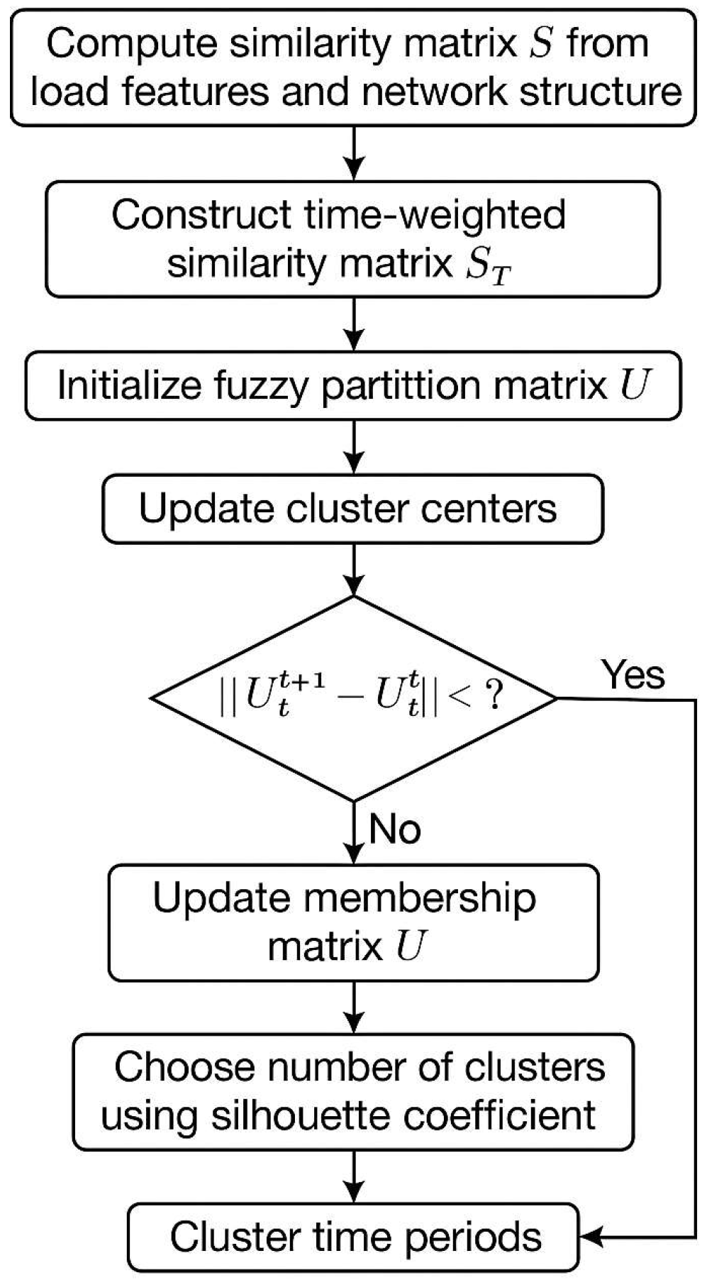
2.4. Solution Process for Load Period Division Method Using Improved Fuzzy C-Means Clustering

The specific steps of the time period partitioning method based on improved fuzzy C-means clustering are as follows, and the flowchart is shown in Figure 1:

Step 1: Comprehensive similarity calculation. Based on the load characteristics of each time period and the optimal network structure for that time period, a feature vector is constructed. According to Equations (1)–(6), the comprehensive similarity $S_{ij}$ between any two time periods i and j is calculated, and a similarity matrix $S\in R^{N\times N}$ is constructed.

Step 2: Introducing time-series smoothing. Based on the original similarity matrix, the information of adjacent time periods is fused according to Equation (7) to construct a time-weighted similarity matrix, which enhances the continuity of similarity in the time dimension and ensures the feasibility and rationality of the partition results in scheduling applications.

Step 3: Initialize clustering parameters. Set initial parameters such as fuzzy index m, maximum iteration times, convergence threshold, etc., and randomly assign initial membership degree $u_{ij}$ to each time period, so that for any time period i, ${\displaystyle {\sum }_{j=1}^C{u}_{ij}=1}$ is satisfied.

Step 4: Similarity weighted center calculation. In each iteration, the similarity matrix is weighted based on the membership degree of the time period, and the fusion similarity $S_{ij}^f$ between time period i and cluster center j is calculated according to Equation (8) as the update basis for each iteration.

Step 5: Update the membership matrix. Update the membership degree $u_{ij}$ based on the fusion similarity, and determine whether the convergence condition is met. Otherwise, continue iterating.

Step 6: Adaptive cluster selection. Evaluate the performance of clustering results under multiple candidate clusters using evaluation indicators such as contour coefficients, and select the optimal cluster number C to improve the quality of partitioning.

Step 7: The final output includes the clustering clusters to which each time period belongs and their corresponding membership degrees, completing the time period partitioning process, which is optimized based on similarity and time information.

3. Power Distribution Network Reconfiguration Mathematical Formulation

This Section describes the tools and methodology that were used to achieve the results presented in this work.

3.1. Objectives Function

The goal of the distribution network reconfiguration problem is to find the optimal configuration. In the present study, the reconfiguration problem is solved taking into consideration active power loss and voltage offset of the distribution network. The objectives of the optimization problem are detailed as follows.

• Active Power Losses Criterion

In the process of transmitting electricity to users, there will inevitably be losses due to factors such as transformers, lines, and the environment. Among them, the network losses of the distribution network account for a large proportion of the losses in the entire transmission system [33,34]. If the loss is too large, not only will the voltage, quality, and stability of the electricity obtained by the user be poor, but it will also bring economic losses to the power supply company. Therefore, in the reconstruction process, the optimization objective is to minimize active power losses, and its mathematical formulation is shown in Equation (11):

$$F_1=\min {\displaystyle \sum _{ij=1}^L{k}_{ij}{R}_{ij}\frac{P_{ij}^2+Q_{ij}^2}{U_{ij}^2}}$$

(11)

where L is the set of all branches in the distribution network, U_ij is the initial voltage of the branch, R_ij is the resistance value of branch ij, K_ij is the opening and closing state variable of the switch on the branch, where one represents the line is closed and zero represents the line is open. P_ij and Q_ij represent the active and reactive power of the incoming branch ij, respectively.

• Voltage Offset Criterion

Voltage offset is a very important indicator for the stable operation of distribution networks. When the load of the distribution network changes, if the voltage offset is too large, it will cause voltage instability in the system, affecting the lifespan of power equipment and the normal operation of the power system [35,36]. Therefore, with the optimization goal of minimizing voltage offset, the voltage of each node in the distribution network can be as close to the rated voltage as possible, thereby improving the stability of the distribution network. The mathematical formulation of this problem can be represented as:

$$F_2=\min {\displaystyle \sum _{i=1}^n\frac{\left|U_i-U_N\right|}{U_N}}$$

(12)

where i is the node number, n is the number of distribution network nodes, U_i represents the voltage of node i, and U_N represents the rated voltage of the system.

The selected multi-objective formulation considers two critical aspects of distribution network performance: active power loss and voltage deviation. Minimizing power losses enhances energy efficiency, while reducing voltage deviation improves power quality and system stability. These two indicators are widely used in existing literature [37,38,39] and are particularly suited for evaluating reconfiguration performance under varying DG and load conditions.

3.2. Constraints

In the study of distribution network reconstruction, in order to achieve reasonable optimization and improvement of the distribution network, a series of constraints needs to be considered.

• Power Flow Constraints

The power flow between loads and power sources in a distribution network is realized through components such as cables, transformers, and switches. The power flow constraint controls the tidal current distribution and power balance of the whole system by considering the electrical parameters of the equipment and components in the power system, which can be expressed as:

$$\left\{\begin{array}{l}{P}_i+P_{DGi}=P_{Li}+U_i{\displaystyle \sum _{i=1}^N{U}_j\left(G_{ij}\cos {\theta }_{ij}+B_{ij}\sin {\theta }_{ij}\right)}\\ Q_i+Q_{DGi}=Q_{Li}+U_i{\displaystyle \sum _{i=1}^N{U}_j\left(G_{ij}\sin {\theta }_{ij}+B_{ij}cos{\theta }_{ij}\right)}\end{array}\right.$$

(13)

where P_i and Q_i represent the active and reactive power flowing to node i. P_DGi and Q_DGi denote the active and reactive output of DG at node i. P_Li and Q_Li denote the active and reactive power of the load at node i. G_ij, B_ij, and θ_ij represent the conductance, susceptance, and voltage phase difference of branch ij, respectively.

• Voltage Constraints

The voltage constraint means that the amplitude of voltage at each node should be limited to a certain range. This constraint can be expressed as:

$$U_{\min }\le U_i\le U_{\max }$$

(14)

where U_i,max and U_i,min are the upper and lower limits of the voltage U_i at node i, respectively.

• Current Constraints

The current carrying capacity of the cable in the system should not exceed the steady-state thresholds as depicted in Equation (15):

$$I_{ij}\le I_{ij}^{\max }$$

(15)

where I_ij is the current transmitted through the branch ij, and I_ij,max represents the maximum current limit in the branch ij.

• DG output constraint

The current carrying capacity of the cable in the system should not exceed the steady-state thresholds as depicted in Equation (16)

$$P_{DG}^{\min }\le P_{DG}\le P_{DG}^{\max }$$

(16)

where $P_{DG}^{\min }$ and $P_{DG}^{\max }$ are the upper and lower limits of DG, respectively.

• Topological constraints

Topological constraints include radial constraint and connectivity constraint:

• Radial constraint: The power supply structure of the distribution network must be radial.
• Connectivity constraint: There must be no islands in the reconfiguration solution, and all nodes must be in a connected state.

4. Optimization Algorithms

Distribution network reconfiguration is a nonlinear integer programming problem, which presents significant challenges in terms of solution complexity and computational cost. Intelligent optimization algorithms are commonly employed to address these challenges, owing to their superior performance in solving optimality-based problems.

The Equilibrium Optimizer (EO) is a novel intelligent optimization algorithm introduced by Afshin Faramarzi et al. [19] in 2020. It is inspired by the control volume of strong hybrid dynamic mass balance in physics and has been successfully applied across various engineering domains, including power systems. EO is particularly suitable for solving the distribution network reconfiguration problem, a complex optimization challenge that requires finding the optimal solution while satisfying multiple constraints. Building on this, the present study proposes an improved version of the Balanced Optimizer algorithm tailored for the distribution network reconfiguration problem.

4.1. Equilibrium Optimizer

EO is inspired by the mass balance equation in physics. In the EO algorithm’s workflow, each particle, along with its concentration, represents an independent individual, with the particles analogous to potential solutions of the optimization problem. Guided by the equilibrium candidate solution, the particles iteratively update their concentrations, converging toward an equilibrium state through the concentration update rule. The parameter design and optimization search process of the algorithm are as follows:

• Initialization and Function Evaluation

EO constructs the initial concentration of the population based on random initialization in the search space and initiates the optimization process. The initial concentration is defined in Equation (17).

$$C_i^{initial}=C_{min}+rand\left(C_{max}-C_{min}\right)\hspace{1em}i=1,2,\dots ,n$$

(17)

where $C_i^{initial}$ denotes the initial concentration vector of the ith particle, C_max and C_min are the upper and lower limit vectors of the optimization variables in the search space, and rand is a random vector between [0, 1], n is the population size.

• Constructing the Equilibrium Pool and Candidates

The equilibrium state represents the algorithm’s final converged solution, which corresponds to the desired global optimum. EO searches for unknown equilibrium states via the Equilibrium Pool. At the start of the iterative process, in the absence of any prior knowledge regarding the equilibrium state, EO selects five particles along with their corresponding concentrations as candidate solutions to guide the search for other particles. The Equilibrium Pool, composed of these candidates, is defined as shown in Equation (18):

$$C_{eq,pool}=\left\{C_{eq(1)},C_{eq(2)},C_{eq(3)},C_{eq(4)},C_{eq(ave)}\right\}$$

(18)

where C_eq(1), C_eq(2), C_eq(3), and C_eq(4) are the four solutions with the best fitness values in the current iteration, and the concentration of the fifth candidate C_eq(ave) is the average of the first four. The probability of these five Candidates being selected is all 0.2.

• Computing Exponential Term (F)

An accurate definition of the exponential term F will assist EO in having a reasonable balance between exploration and exploitation.

$$\mathit{F}=a_1\mathrm{sign}\left(\mathit{r}-0.5\right)\left[e^{-\lambda t-1}\right]$$

(19)

where a₁ is a constant value that controls exploration ability by amplifying the concentration change; λ and r are the random vectors in [0, 1] with the same dimension as the optimization space dimension; and sign(r − 0.5) indicates the control of the direction of exploration and exploitation.

The time parameter t is an iterative function that decreases as the number of iterations increases and is updated as shown in Equation (20):

$$t={\left(1-{\displaystyle \frac{Iter}{Max\_Iter}}\right)}^{\left(a_2{\displaystyle \frac{Iter}{Max\_Iter}}\right)}$$

(20)

where a₂ is a constant value that controls exploitation ability, Iter is the current number of iterations, and Max_Iter is the defined maximum number of iterations.

• Computing Generation Rate (G)

The Generation Rate G is an important parameter to provide the exact solution by improving the exploitation process, which helps EO to accelerate the convergence to the optimal solution in later iterations. The value of G is shown as a first-order exponential decay process, defined as shown in Equations (21)–(23):

$$G=G_0{e}^{-\lambda \left(t-t_0\right)}=G_{0}F$$

(21)

$$G_0=GCP\left(C_{eq}-\lambda C\right)$$

(22)

$$GCP=\left\{\begin{array}{l}0.5r_1\hspace{1em}\hspace{1em}{r}_2\ge GP\\ 0\hspace{1em}\hspace{1em}\hspace{1em} r_2<GP\end{array}\right.$$

(23)

where λ is the decay constant, r₁ and r₂ are both random numbers between [0, 1], and the Generation Rate Control Parameter (GCP) indicates the probability that the generation term contributes to the update process and is determined by the Generation Probability (GP). When GP = 1, no generation rate will be involved in the optimization process, and when GP = 0, the generation rate will always be involved in the process.

• Concentrations Update and Iterative Optimization

Guided by the candidate solutions, each particle iteratively updates its concentration using the update rule of EO, as shown in Equation (24). EO compares the fitness value of each particle in the current iteration with that of the previous generation, retaining the particle with the superior fitness value. The optimization process terminates when the maximum number of iterations is reached.

$$C=C_{eq}+\left(C-C_{eq}\right)F+{\displaystyle \frac{G}{\lambda V}}\left(1-F\right)$$

(24)

4.2. Feasible Solution Determination

In the distribution network reconfiguration problem, the optimal combination of switch action sequences must satisfy the radial and connectivity constraints of the network, ensuring that no islanding or ring network formation occurs. However, during the search process of intelligent optimization algorithms, the randomness in the combination of switch opening and closing states leads to a high number of infeasible solutions and low-quality feasible solutions, thereby increasing the computational cost of reconfiguration. To address this, a feasible solution determination model, JR, based on adaptive ordered loops, is proposed. This model helps to avoid infeasible solutions generated during the reconfiguration process and eliminates inferior solutions with high fitness values, thereby compressing the solution space.

4.2.1. Network Coding Based on Basic Ring Matrix

Power networks typically use two distinct types of switching structures: sectionalizing switches (S.S.s) and tie switches (T.S.s). During the reconfiguration process, T.S.s are normally open, while S.S.s are normally closed. Following the reconfiguration, certain switches may change their positions based on the optimization results.

Distribution network design considers the loop formed by each T.S. and several S.S.s as the basic ring. For instance, in the IEEE 33-bus distribution network, five interconnection switches correspond to five basic loops. In this study, the basic loop matrix is defined as H, based on the decimal encoding of all branches within the distribution network loop.

$$\mathit{H}={\left(H_{lk}\right)}_{L\times K}$$

(25)

where L is the number of basic loops, which is the same as the number of contact switches, K is the maximum value of the number of branches contained in all basic loops, and the rows with the number of segmented switches less than K are completed with zeros. In this paper, we utilize the natural number encoding to represent the branch H_lk; H_lk is a non-zero integer, which represents the number of the branch where the kth switch of the lth basic ring is located; the matrix H₀ represents the initial network topology before reconfiguration.

Taking the IEEE 33-bus distribution network as an example, its basic ring matrix H is presented in Equation (26), and the correspondence between its basic rings and branches is displayed in

Table 1. The correspondence between basic loops and switches.

Basic Ring	Branches	T.S.	Number
1	s2, s3, s4, s5, s6, s7, s20, s19, s18	s33	1~10
2	s9, s10, s11, s12, s13, s14	s34	1~7
3	s2, s3, s4, s5, s6, s7, s8, s9, s10, s11, s21, s20, s19, s18	s35	1~15
4	s6, s7, s8, s9, s10, s11, s12, s13, s14, s15, s16, s17, s32, s31, s30, s29, s28, s27, s26, s25	s36	1~21
5	s3, s4, s5, s25, s26, s27, s28, s24, s23, s22	s37	1~11

. The topology of the IEEE 33-bus distribution system [14] is shown in Figure 2.

$$\mathit{H}=\left(\begin{array}{cccccccccccccccccccc}2& 3& 4& 5& 6& 7& 20& 19& 18& 0& 0& 0& 0& 0& 0& 0& 0& 0& 0& 0\\ 9& 10& 11& 12& 13& 14& 0& 0& 0& 0& 0& 0& 0& 0& 0& 0& 0& 0& 0& 0\\ 2& 3& 4& 5& 6& 7& 8& 9& 10& 11& 21& 20& 19& 18& 0& 0& 0& 0& 0& 0\\ 6& 7& 8& 9& 10& 11& 12& 13& 14& 15& 16& 17& 32& 31& 30& 29& 28& 27& 26& 25\\ 3& 4& 5& 25& 26& 27& 28& 24& 23& 22& 0& 0& 0& 0& 0& 0& 0& 0& 0& 0\end{array}\right)$$

(26)

4.2.2. Feasible Solutions Determination Based on Basic Ring Matrix

During the reconfiguration process, T.S.s are normally open, and S.S.s are normally closed. After reconfiguration, some switches change their positions based on the optimization results [12]. Distribution network reconfiguration essentially involves the opening and closing of switches. When all switches are closed, the distribution network topology can be represented as a connected graph, denoted as G. By specifying that the total number of branches equals the difference between the total number of nodes and the number of root nodes in the distribution network, the occurrence of a large number of infeasible solutions can be avoided, as shown in Equation (27):

$${\displaystyle \sum _{ij\in H}{h}_{ij}=n_b-n_s,h_{ij}\in \left\{0,1\right\}}$$

(27)

where H is the set of branches of the above distribution network, h_ij is the open and closed state of the branch, with zero denoting disconnection and one denoting closure, and n_b and n_s denote the total number of nodes and the number of root nodes in the distribution network, respectively.

In actual distribution networks, common branches exist between loops, which are shared by multiple loops simultaneously. If two switches are disconnected at the same time on a common branch, it may result in the formation of an island, as illustrated in Figure 3. To address this issue, the following three provisions are established: at most, one disconnection is allowed on the common branch L_mn between any loops m and n, as shown in Equation (28); at most, one non-public branch can be disconnected, as shown in Equation (29); and if n branches are connected at node j, then no more than n − 1 branches can be disconnected at this node, as shown in Equation (30).

$${\displaystyle \sum _{\left(i,j\right)\in L_{mn}}1-h_{ij}\le 1,L_{mn}=L_m\cap L_n}$$

(28)

$${\displaystyle \sum _{\left(i,j\right)\in C_{L_m}{L}_{mn}}{h}_{ij}\ge n_{L_m}-1,\forall m\in L,\forall n\in L}$$

(29)

$${\displaystyle \sum _{\left(i,j\right)\in K_j}{h}_{ij}\ge 1,\forall j\in \left\{1,2,\dots ,n_b\right\}}$$

(30)

where L_m denotes the set of branches in the mth loop, $n_{L_m}$ denotes the number of branches in the mth loop, L denotes the total number of loops, and K_j denotes the set of branches connected to the jth node.

The method described above effectively avoids infeasible solutions in the reconfiguration process. However, due to the inherent randomness in the search process of intelligent optimization algorithms, a large number of inferior solutions remain in the solution space, specifically low-quality feasible solutions with high fitness values. The overall lower quality of solutions leads to an increased reconfiguration time. Therefore, this paper calculates the power moment based on the real-time load of each node, removes duplicate branches through branch verification, and generates an adaptive ordered loop feasible solution matrix, denoted as JM. The specific process is as follows:

Step 1: Find the repeated branch S_i in the basic ring matrix H, with its repetition number Nr, where S_i appears in the basic ring matrix, and find all positions H_l1k1, H_l2k2, …, H_lNrkNr. Assuming that the switch corresponding to the repeated branch S_i is disconnected and the other switches are closed, with its end node being Ne_i, the backflow path formed by the set of branches and nodes from node Ne_i to the source point of the loop is denoted as L_i (i = 1, 2, …, Nr).

Step 2: Calculate the impedance distance Z_ni, which is the sum of all branch impedances of the countercurrent path L_i, as shown in Equation (31):

$$Z_{ni}={\displaystyle \sum _{b_j\in L_j}{Z}_{b_j}}$$

(31)

Step 3: Calculate the generalized load W_ni, which is the product of the impedance distance Z_ni from the node to the origin and the conjugate of the node load, as shown in Equation (32):

$$W_{ni}=Z_{ni}\stackrel{\ast }{S_{ni}}$$

(32)

Step 4: Calculate the power moment T_i of node Ne_i and set the minimum value to T_i,min. The power moment T_i is the real part of the sum of the generalized loads W_ni of all nodes on the countercurrent path L_i, as shown in Equation (33):

$$T_i=\mathrm{Re}\left({\displaystyle \sum _{n_i\in L_i}{W}_{n_i}}\right)$$

(33)

Step 5: According to the power moment calculation, perform branch verification without changing the original branch order and remove duplicate branches. Make the following modifications to the basic loop matrix H to generate an ordered loop feasible solution matrix JM: in the basic loop matrix H, only the branch S_i is retained in the loop where the minimum power moment is located, while the other branches are reassigned to zero in the basic loop matrix H, as shown in Equation (34). If there are branches located in different basic loops but with the same loop-breaking effect, only the branches far from the root node are retained, and the other branches are reassigned to zero in the basic loop matrix H.

$$m_{idjd}=\left\{\begin{array}{l}U\hspace{1em}\hspace{1em}{T}_d=T_{d’}\\ 0\hspace{1em}\hspace{1em}{T}_d\ne T_{d’}\end{array}\right.$$

(34)

Step 6: Repeat steps 1 to 4 until all repeated branch verifications are completed, ending the loop and outputting the adaptive ordered loop feasible solution matrix JM.

$$JM=\left(\begin{array}{cccccccccc}2& 3& 4& 5& 6& 7& 33& 20& 19& 18\\ 34& 14& 13& 12& 0& 0& 0& 0& 0& 0\\ 21& 35& 11& 10& 0& 8& 0& 0& 0& 0\\ 15& 16& 17& 36& 32& 31& 30& 29& 0& 0\\ 25& 26& 27& 28& 37& 24& 23& 22& 0& 0\end{array}\right)$$

(35)

Through branch verification, a significant number of inferior solutions that satisfy topological constraints can be filtered out, allowing the optimal solution to be more easily located within the solution space. The feasible solution judgment model JR, based on the adaptive ordered loop, eliminates many inferior solutions through branch verification, thereby narrowing the range of feasible solutions and further enhancing the overall quality of the solution space. This not only improves the efficiency of the reconfiguration process but also facilitates the algorithm’s ability to search for the optimal solution. The detailed steps of the proposed method are presented in Algorithm 1.

Algorithm 1: Pseudo code of Generate Adaptive Ordered Loop Feasible Solution Matrix JM
Input:	Basic loop matrix H, branch impedance Z, node equivalent load $\stackrel{\ast }{S}$
Output:	Adaptive ordered loop feasible solution matrix JM
1:	for each repeated branch Si in H do
2:	Determine the number of repetitions Nr and positions Hl1k1, Hl2k2, ……, HlNrkNr
3:	Construct reverse path Li from end node Nei to source node
4:	Compute total impedance on path Li: Zni = ∑(Zbj), ∀bj∈Li
5:	Compute generalized load: $W_{ni}=Z_{ni}\stackrel{\ast }{S_{ni}}$
6:	Compute power matrix at node Nei: Ti = Re(∑(Wni)), ∀ni∈Li
7:	Identify path wnith minimum power value Tmin
8:	for each position of Si in H do
9:	if Td = Tmin then
10:	midjd = U // Retain branch
11:	else
12:	midjd = 0 // Remove redundant branch
13:	end if
14:	end for
15:	end for
16:	Repeat steps 1–15 until all repeated branches are validated
17:	Output ordered feasible decoding matrix JM

4.3. The Proposed Improved Equilibrium Optimizer Algorithm

To address the limitations of the standard Equilibrium Optimizer (EO), such as slow convergence, tendency to fall into local optima, and Suboptimal Balance between Exploration and Exploitation, this study develops an Improved Equilibrium Optimizer (IEO) by introducing several targeted modifications. First, a Tent chaotic map is applied during the initialization phase to enhance population diversity and avoid premature convergence. Second, an elite non-dominated sorting mechanism is embedded to allow the optimizer to handle multiple objectives without requiring explicit scalarization, thereby preserving the integrity of each objective function. Additionally, a stochastic mutation strategy is adopted to increase the global exploration capability of the algorithm, and a binomial crossover operator is incorporated to promote information exchange and accelerate convergence. These improvements are seamlessly integrated into the EO framework, collectively contributing to enhanced search efficiency, solution diversity, and convergence stability. The following subsections describe the specific design and rationale of each enhancement in detail.

4.3.1. Population Initialization Based on Tent Mapping

The initial population significantly influences the performance of the Intelligent Optimization Algorithm. In EO, the initial population concentration is generated based on the random vector rand in Equation (17). However, this completely random initialization cannot ensure a uniform distribution of the initial population within the search space. Additionally, if the initial population is overly concentrated, it may lead to local optimization, hindering the search for the optimal solution in the distribution network reconfiguration problem.

Chaotic sequences exhibit characteristics such as randomness, orderliness, and transversality. The Tent Chaotic Map is capable of quickly generating uniform random sequences, offering advantages over other mapping algorithms. In this study, the Tent Chaotic Map is employed to improve the initialization of the EO population, ensuring a well-distributed initial population that covers the search space effectively with good uniformity and diversity. This enhancement improves both the performance and efficiency of EO in the early stages of the process. The expression is given in Equation (36), and the population initialized using the Tent Chaotic Map is shown in Equation (37):

$$Y_{t+1}=\left\{\begin{array}{l}2Y_t\hspace{1em}\hspace{1em}\hspace{1em} 0\le Y_t<0.5\\ 2\left(1-Y_t\right)\hspace{1em}0.5\le Y_t\le 1\end{array}\right.$$

(36)

$${\mathit{C}}_i^{initial}={\mathit{C}}_{min}+Y_i\left({\mathit{C}}_{max}-{\mathit{C}}_{min}\right)\hspace{1em}i=1,2,\dots ,n$$

(37)

where C_max and C_min denote the upper and lower bounds of the search space, respectively.

4.3.2. Non-Dominated Sorting with Elite Strategy

To enable EO to address the multi-objective distribution network reconfiguration problem, this study incorporates Non-Dominated Sorting (NDS) with an Elite Strategy.

First, evaluate each solution based on all objective functions in the target space and use the NDS mechanism to identify non-dominated solutions. In each iteration, compare the new and old equilibrium concentrations. If the new equilibrium concentration dominates the old one, replace the old concentration with the new one, and store the non-dominated solutions found in that iteration in an external archive.

An elite strategy is introduced to retain the best individuals from previous generations and incorporate them into the next generation, working alongside the non-dominated sorting. This strategy expands the sampling space, accelerates the algorithm’s execution, and, to some extent, prevents the loss of solutions on the Pareto frontier.

The external archive is updated by comparing the non-dominated solutions with the new candidates. When the number of non-dominated solutions exceeds the archive size, the crowding distance for each objective function is calculated for each individual in the non-dominated layer, as shown in Equation (38). The individual with the smallest crowding distance is then removed iteratively.

$$i_d={\displaystyle {\sum }_{j=1}^m\left(\left|f_j^{i+1}-f_j^{i-1}\right|\right)}$$

(38)

In the proposed IEO framework, the integration of a non-dominated sorting mechanism not only ensures diversity but also effectively guides the search toward the Pareto front. This strategy allows the algorithm to maintain a set of trade-off solutions across multiple objectives.

Unlike conventional approaches that rely on scalarization through weighted summation, the IEO adopts a Pareto-based multi-objective optimization strategy. Instead of combining objectives such as power loss and voltage deviation into a single composite function with predefined weights, the algorithm directly optimizes these criteria in parallel. During the iterative process, elite non-dominated sorting is employed to evaluate solution dominance and maintain a high-quality and diverse Pareto front.

This approach eliminates the need for subjective weight selection and preserves the intrinsic trade-off relationships between conflicting objectives. As a result, the optimization process produces a well-distributed set of solutions, each representing a distinct balance between power loss minimization and voltage profile improvement. This not only enhances the fairness and flexibility of the reconfiguration scheme but also improves its interpretability and practical applicability under varying operational priorities.

4.3.3. Stochastic Differential Mutation Strategy

EO balances global and local search capabilities through a unique Equilibrium Pool mechanism and a concentration update rule. However, these optimization methods introduce limitations in applying EO to the distribution network reconfiguration problem. First, during the Equilibrium Pool stage, candidate selection is based solely on fitness values, which may lead to candidates being in similar positions, reducing population diversity. Additionally, EO relies exclusively on the concentration update rule for individual updates, causing all concentration vectors to converge towards candidates with better fitness values during iterations. This accelerates convergence, increasing the risk of falling into local optima. Moreover, EO lacks an effective strategy to escape local optima, limiting its ability to find the global optimum.

To address the aforementioned issues, this study proposes the Stochastic Differential Mutation Strategy, inspired by the DE/target-to-best/1 mutation strategy in Differential Evolutionary Algorithms. The Stochastic Differential Mutation Strategy combines stochastic selection with a local random wandering mechanism, using the difference vectors and equilibrium candidates of EO as two perturbation terms to generate mutation recombinants. The strategy is defined as shown in Equation (39):

$$V_{ij}=C_{ij}+F1\left(C_{eq(j)}-C_{ij}\right)+F2\left(C_{r1(j)}-C_{r2(j)}\right)$$

(39)

where V_ij denotes the jth component of the variation vector V_i; C_ij denotes the jth component of the current solution vector C_i; C_eq is a randomly selected candidate in the Equilibrium Pool; C_r1 and C_r2 are two solutions randomly selected in the population; and the scale factors F1 and F2 are positive control parameters used to scale the perturbation term in [0.5, 1]. The perturbation term multiplied by F1 is an arithmetic recombination operation, and the perturbation term multiplied by F2 is a differential mutation operation. Therefore, what is generated in the stochastic global mutation strategy is basically a mutational recombinant rather than a pure mutation.

The concentration of particles in an iteration has a certain probability of undergoing mutation. In the distribution network reconfiguration problem, this probability is described in Equation (40):

$$P_m=P_{\min }+\left(P_{\max }-P_{\min }\right)\times {\displaystyle \frac{t}{Max\_Iter}}+P_c$$

(40)

where P_m is the mutation rate of an individual at the tth generation; P_max and P_min are the maximum and minimum mutation rates of an individual, respectively; Max_Iter is the maximum number of iterations of the population; and P_c is a constant to be determined, the value of which is dependent on the period in which the distribution network is reconfigured.

The stage of the distribution network reconfiguration is judged based on the reduction Re of the active power loss in the three consecutive optimal reconfiguration results. When $Re>\alpha \left(\alpha \in \left[3\%,5\%\right]\right)$, it is judged to be the pre-reconfiguration stage. Because of the large difference in particle concentration in the pre-iteration period, the Equilibrium Pool mechanism is utilized as much as possible to its own advantage, so $P_c=0.03$. When $Re\le \alpha$, it is judged as the later reconstruction stage. The particle concentration difference is smaller during the later stage of iteration; thus, the ability of the algorithm to jump out of the local optimum should be improved, so $P_c=0.1$.

This study designs a variation strategy for JR, a feasible solution judgment model based on adaptive ordered loops. First, real number encoding is used to represent the disconnected circuits C_ij within the concentration particle Ci in the EO algorithm. The concentration particle Ci represents a specific solution generated in a given iteration, and its dimensions match the solution space dimensions of the distribution network reconfiguration. Cij represents one dimension of the solution, which is derived from the adaptive ordered loops feasible solution matrix JM, with each dimension corresponding to one of the loops in the matrix (i.e., j is constantly equal to l). Each basic loop is set as a variable, and each variable corresponds to a branch encoding representing the switch number in the loop. The variable takes values within the range of the number of switches in the loop, and when encoded, it indicates whether the corresponding branch’s switch is turned on. For each independent loop, a variation is applied to the intra-ring number i of branch Cij. If the variant number exceeds the maximum number of branches kj in the loop, the result is divided by kj, and the remainder is mapped back to the original loop as the final variant branch, following the property that the first branch is connected to the first branch of the loop.

Introducing the stochastic differential variational strategy into the standard EO algorithm not only facilitates a smooth transition between the pre-intermediate exploration and development phases but also increases perturbation near the extremum during the algorithm’s iterations. This helps prevent stagnation in local optima, contributing to the diversification of the Pareto frontier and enhancing the algorithm’s ability to find optimal solutions, thus avoiding low-quality local optima. The integration of the proposed adaptive ordered loop-based feasible solution judgment model JR with the improved EO algorithm further enhances both the solution efficiency and the optimal solution search capability of the reconfiguration algorithm.

4.3.4. Binomial Crossover and Selection Operation

To further increase the population’s potential diversity of EO, this study adopts the binomial crossover operation, in which the dimensional components of the mutation concentration V_i and the current concentration C_i are randomly reorganized by a crossover operation. The solution individual after the mutation and crossover operation is defined as the trial vector U_i, and the scheme may be outlined as:

$$U_{ij}=\left\{\begin{array}{l}{V}_{ij} \mathrm{if} \left(CR\ge rand or j=j_{rand}\right)\\ C_{ij} \mathrm{otherwise}\end{array}\right.$$

(41)

where CR is the crossover probability between [0, 1], and j_rand is the dimension identity randomly generated within [1, D]. For each dimension j, a random number rand is generated between [0, 1), and if its value is less than CR, then the jth dimension of U_i comes from the jth dimension of Vi; otherwise, from the jth dimension of C_i.

In this case, the number of parameters inherited from the mutation vector will have an approximate binomial distribution. The crossover must occur if the current dimension j is equal to j_rand. This rule ensures that the trial vector U_i obtains at least one component from the mutation vector V_i, thereby preventing them from being identical. The scheme ensures the generation of new individuals and mitigates the risk of evolutionary stagnation within the population.

Finally, the selection operation will apply the principle of “survival of the fittest” to the trial vector U_i and the current vector C_i. The individuals with better fitness values in the current generation G will be saved in the next generation of the population, as shown in Equation (42).

$$C_{i,G+1}=\left\{\begin{array}{l}{U}_{i,G}\hspace{1em}\hspace{1em}if\hspace{1em}f\left(U_{i,G}\right)\le f\left(C_{i,G}\right)\\ C_{i,G}\hspace{1em}\hspace{1em}otherwise\end{array}\right.$$

(42)

4.4. Algorithm Comparison and Complexity

The proposed Improved Equilibrium Optimizer (IEO) introduces several tailored enhancements to address the challenges of dynamic distribution network reconfiguration. Unlike the standard EO algorithm, which employs uniform random initialization and lacks explicit feasibility enforcement, IEO incorporates Tent chaotic mapping to enhance population diversity and utilizes an adaptive ordered loop-based feasibility judgment model to ensure compliance with radial topology and operational constraints. In contrast to widely used multi-objective algorithms like NSGA-II, IEO incorporates a more flexible variation strategy through stochastic mutation and binomial crossover, enabling it to better maintain population diversity and avoid premature convergence. While classical metaheuristics often focus solely on optimization, the IEO is embedded within a broader framework that includes load period clustering and feasibility assessment, making it more suitable for handling the temporal variability and complexity inherent in active distribution networks. These design choices collectively enhance the robustness and applicability of the proposed method.

The computational complexity of the proposed Improved Equilibrium Optimizer (IEO) is influenced by the number of individuals N, the dimension of the decision variable D, and the number of iterations T. For each iteration, all individuals undergo chaotic initialization, feasibility evaluation, non-dominated sorting, mutation, and crossover. Therefore, the overall time complexity of IEO can be approximated as:

$$O\left(N\cdot D\cdot T\right)+O\left(N\cdot \log N\right)$$

(43)

where the first term accounts for the core evolutionary operations, and the second term arises from elite sorting and ranking procedures. Additionally, the complexity of the feasibility judgment model and clustering procedure is kept linear with respect to the number of scenarios and time intervals due to the offline precomputation structure. This ensures that the overall framework remains computationally scalable even for medium-sized distribution networks such as the IEEE 69-bus system.

4.5. The Flow of the Improving Equilibrium Optimizer

The flow of the improved EO algorithm applied to the multi-objective distribution network reconfiguration problem obtained according to the above improvement strategy is shown in Figure 4, and the specific steps are described as follows.

Step 1: Input distribution network nodes, branch data, DG-related parameters and parameters of the improved EO algorithm including population size, upper and lower bound vectors of optimization variables C_max and C_min, maximum iteration number Max_Iter, weight constant coefficient a₁ for global search, weight constant coefficient a₂ for local search, generation probability parameter GP, etc.

Step 2: Introduce the feasible solution judgment model JR based on adaptive ordered loops, and generate the adaptive ordered loop feasible solution matrix JM.

Step 3: Perform stochastic uniform initialization of the population pop according to Equation (37) to construct the initial concentration of the population with iteration number Iter = 1.

Step 4: Perform the trend calculation for all individuals, and find the fitness values F₁(C_i), F₂(C_i) of the individuals in the population according to the objective function, where C_i is the concentration vector of the ith individual in the current population.

Step 5: Evaluate each solution with all the objective functions in the objective space, apply the NDS mechanism to judge the dominance relationship of the concentration particles, and at the same time, introduce the elite strategy, and calculate the crowding distance for the individuals in each non-dominated layer, and select the appropriate individuals to be deposited in the external archive according to Equation (38).

Step 6: Select candidates based on the sorted results and construct the equilibrium pool C_eq,pool.

Step 7: Update the individuals using the Equation (24) concentration update formula under the guidance of the candidates in the balanced pool. The stochastic differential mutation strategy of Equation (39) and the binomial crossover strategy of Equation (41) are introduced to perform the mutation and crossover of particles according to the mutation probabilities in different periods of the distribution network reconfiguration, and the concentration of particles generated is U_i.

Step 8: The selection operator based on Equation (42) will perform a winnowing operation on the test concentration vector U_i and the current concentration vector C_i, and take the individual with the better adaptation value in the current Gth generation to be saved in the next generation population.

Step 9: Judge whether the maximum number of iterations is satisfied, and if not, repeat steps 3 to 7; if satisfied, terminate the iteration and output the optimal reconstruction solution.

5. Case Study and Result

To assess the effectiveness of the proposed algorithm, comprehensive case studies on IEEE test systems are carried out. The IEEE 33-bus system is employed to demonstrate the superiority of the proposed algorithm, while the IEEE 69-bus system is used to validate its scalability.

5.1. Basic Parameter

The topology of the IEEE 33-bus distribution system [14] is shown in Figure 2. The system has a standard load value of 3175 kW, a rated voltage of 12.66 kV, and a reference power of 10 MW. The line length is calculated based on branch impedance conversion. DG units are connected to nodes 9, 18, 19, 21, and 32. Wind turbines with a rated power of 500 kW are connected to nodes 9, 18, and 21. These turbines have a cut-in wind speed of 3 m/s, a rated wind speed of 15 m/s, and a cut-off wind speed of 20 m/s. Nodes 19 and 32 are connected to photovoltaic units with a total array area of 7000 m² and a conversion efficiency of 19.8%. The wind speed v and solar intensity r for each time period are taken from reference [12], with a load forecasting error of ±10%. The fluctuation range caused by forecasting errors in wind speed and light intensity is [0.9, 1.1] p.u. The total number of switch actions during the reconstruction period is limited to no more than 20, with no individual switch action occurring more than 4 times.

The simulation environment is as follows: an Intel^® Core™ i5-7400T processor (Intel Corporation, Santa Clara, CA, USA) with a clock speed of 2.40 GHz and 8 GB of RAM. The relevant algorithms were implemented and validated using MATLAB R2021a. The specific algorithm parameters are as follows: the maximum number of iterations, Max_Iter, is set to 100, and the probability parameter GP is 0.5. To balance global and local search capabilities in the reconstruction process, the weight constant for global search, a₁, is set to 2, and the weight constant for local search, a2, is set to 1. Each algorithm was independently run 100 times in this study.

5.2. Division of Load Periods

Before presenting the clustering results, it is essential to clarify their role in driving the dynamic reconfiguration model. In the proposed framework, the improved fuzzy C-means (FCM) clustering algorithm introduced in Section 2 is not merely used to segment daily load profiles, but also directly informs the reconfiguration decisions of the distribution network. Specifically, the 24 h load data are divided into multiple representative periods, each treated as an independent reconfiguration scenario. The average load of each cluster is used as the input of the optimization model, enabling the generation of time-specific network topologies. This strategy effectively transforms the static reconfiguration problem into a dynamic, time-aware process, allowing the system to adapt to fluctuations in both load demand and DG output throughout the day.

To support this, the enhanced FCM algorithm performs time segmentation based on both temporal characteristics and network structural similarity. The reliability and consistency of the clustering results provide a solid foundation for the subsequent optimization and performance evaluation.

To determine the optimal number of clusters, two commonly used evaluation indicators—the elbow method and the silhouette coefficient—are employed [40,41,42,43]. The elbow method assesses the reduction in the Sum of Squared Errors (SSE) by increasing, identifying the point at which adding more clusters yields diminishing returns. The silhouette coefficient, meanwhile, evaluates the cohesion and separation of clustering results, with values closer to 1 indicating better-defined clusters.

Using these metrics, the improved fuzzy C-means clustering method achieves accurate and interpretable load period segmentation. The corresponding SSE curve is shown in Figure 5, and the clustering results are visualized in Figure 6.

The experimental results indicate that as the number of clusters increases, the SSE value decreases progressively, but the decline significantly slows around k = 5, forming a typical ‘elbow’ shape. This suggests that k = 5 strikes a good balance between maintaining intra-class consistency and inter-class differentiation. Additionally, the silhouette coefficient reaches a local maximum at k = 4, and although it slightly decreases at k = 5, it remains high, indicating that the clustering structure retains good separability.

Considering both the time division accuracy and scheduling feasibility, k = 5 was ultimately chosen as the optimal number of clusters, striking a balance between the rationality of load characteristic division and the practical applicability of distribution network reconfiguration. The time period is divided into five clusters, with the periods in each cluster shown in Figure 7. Clusters 1, 2, 3, 4, and 5 correspond to the time periods 00:00–08:00, 08:00–13:00, 13:00–17:00, 17:00–21:00, and 21:00–24:00, respectively.

5.3. Comparison and Analysis of Dynamic Reconfiguration Results

To assess the feasibility, effectiveness, and superiority of the proposed fuzzy C-means clustering time division method and the improved EO algorithm for active distribution network reconstruction, three schemes are set up for comparative analysis:

Scheme 1: No network reconstruction, disconnect all contact switches at all times. Scheme 2: Static reconstruction using the improved EO algorithm proposed in this study, i.e., performing reconstruction once per day. Scheme 3: Dynamic reconstruction optimization based on the method proposed in this study. The reconstruction results for each scheme are presented in

Table 2. Comparison and Analysis of Dynamic Reconfiguration Results in IEEE33.

Scheme	Time Interval	Disconnected Branches	Loss/kWh	Voltage Deviation/p.u.
Scheme 1	All time	s33-s34-s35-s36-s37	1320.4	25.1
Scheme 2	All time	s7-s14-s9-s36-s37	961.7	18.6
Scheme 3	00:00–08:00	s7-s34-s9-s31-s37	729.3	16.1
	08:00–13:00	s7-s14-s9-s31-s37
	13:00–17:00	s7-s14-s10-s32-s28
	17:00–21:00	s7-s14-s9-s32-s30
	21:00–24:00	s7-s14-s9-s32-s28

.

From the comparison between Scheme 1 and Scheme 2 in Table 2, it is evident that without any reconstruction strategy, the distribution network remains in its initial state, with no section switches in operation. This lack of optimization leads to high energy consumption and significant voltage deviation. However, after applying the improved EO algorithm, system performance improves substantially. Network loss decreases by about 27.2%, from 1320.4 kWh to 961.7 kWh, and voltage deviation reduces by 25.9%, from 25.1 p.u. to 18.6 p.u. This shows that even with a single optimization per cycle, the improved EO algorithm can achieve notable performance gains.

Further comparison of Scheme 2 and Scheme 3 reveals that while Scheme 2 effectively reduces network loss and voltage deviation, its static nature limits the potential for dynamic topology adjustment within the allowed switching range. Scheme 3, however, introduces a load period clustering method, dividing the day into representative periods and optimizing reconstruction for each. As a result, network loss further decreases to 729.3 kWh, a 24% reduction compared to Scheme 2, while voltage deviation drops to 16.1 p.u., a 13% improvement, demonstrating the advantages of dynamic reconstruction.

In summary, the proposed method outperforms Scheme 1 and Scheme 2 in reducing distribution network losses, improving node voltage deviations, and enhancing power quality. This indicates that the dynamic reconstruction strategy not only optimizes power flow distribution but also enhances the consumption capacity of distributed generation, balancing active and switching losses, and improving the system’s economy and reliability. The changes in network loss values for each period in the three schemes are shown in Figure 8.

From Figure 8, it is evident that Scheme 3 significantly reduces network loss compared to Scheme 1 and Scheme 2 in all time periods. The most substantial reduction occurs during the 19–21 h period, which is the peak load period of the day. During this time, residential, commercial, and industrial loads reach their highest levels, while photovoltaic output drops to nearly zero, and wind turbines are unable to fully meet the demand, leading to line overload and increased network losses. The dynamic reconstruction in Scheme 3 effectively mitigates these losses, improving the overall economic efficiency of the system.

Figure 9, Figure 10 and Figure 11 show the voltage distribution at each node across the time periods for the three schemes. These figures illustrate the voltage profiles of all nodes over 24 time periods using a 3D surface plot, where the color gradient reflects the voltage magnitudes. The horizontal axes represent node indices and time periods, while the vertical axis indicates the corresponding voltage values. As illustrated in Figure 11, the dynamic reconstruction method proposed in this study results in an overall increase in node voltage compared to the other two schemes. Voltage fluctuations are smaller, and the voltage levels are higher. Specifically, the lowest voltage has increased from 0.928 p.u. before reconstruction to 0.949 p.u. This demonstrates an overall improvement in network voltage, with a more stable and uniform distribution, enhancing both power quality and grid safety, while maintaining economic operation.

This article introduces a random difference mutation strategy and a binomial crossover strategy into the iteration process of the EO algorithm to enhance the diversity of the candidate set in the entire equilibrium pool. The improved algorithm exhibits fast optimization and ensures population diversity throughout the process. While the standard EO algorithm tends to converge to local optima within the same number of iterations, the improved EO algorithm overcomes these limitations, enabling faster convergence toward the global optimal solution. In conclusion, the enhanced EO algorithm offers significant advantages in terms of optimization efficiency and solution quality.

5.4. Comparative Analysis of Different Algorithms

To comprehensively evaluate the performance of the proposed Improved Equilibrium Optimizer (IEO) in solving the distribution network reconfiguration problem, this study conducts comparative experiments against several widely used metaheuristic algorithms, including Particle Swarm Optimization (PSO), Grey Wolf Optimization (GWO), Harris Hawk Optimization (HHO), the standard Equilibrium Optimizer (EO), and the Non-dominated Sorting Genetic Algorithm II (NSGA-II).

To ensure fair and objective comparisons, all benchmark algorithms (including PSO, GWO, HHO, and NSGA-II) were executed under identical experimental settings. The population size, maximum number of iterations, and evaluation metrics were uniformly set across all methods. Moreover, for each algorithm, parameter settings were either selected based on widely accepted literature defaults or fine-tuned through preliminary experiments to ensure optimal performance without bias. All algorithms were independently run 30 times, and the best, worst values were recorded for performance analysis.

This unified experimental configuration eliminates discrepancies in runtime or resource allocation, thereby validating the reliability and fairness of the comparative results.

In order to provide a comprehensive assessment, this paper compares both the optimal and worst-case results for each algorithm, as shown in

Table 3. Comparison of solution situations of different algorithms.

Algorithm	Best Case			Worst Case
	Disconnected Branches	Loss/kW	Minimum Voltage/p.u	Disconnected Branches	Loss/kW	Minimum Voltage/p.u
PSO	7-9-14-32-37	139.551	0.938	7-13-16-28-35	156.872	0.071
GWO	7-9-14-32-37	139.551	0.938	7-14-21-26-32	143.219	0.067
HHO	7-9-14-32-37	139.551	0.938	13-17-20-21-28	186.955	0.072
NSGA-II	7-9-14-32-37	139.551	0.938	7-10-15-21-26-32	149.328	0.069
EO	7-9-14-32-37	139.551	0.938	7-13-20-28-34	157.276	0.070
Improved EO	7-9-14-32-37	139.551	0.938	7-11-17-28-34	147.643	0.067

. The results reveal that, even in the worst-case scenario, the switch scheme produced by the improved EO algorithm outperforms the other algorithms in terms of network loss and minimum voltage.

This paper also evaluates the performance of different algorithms by comparing their convergence behaviors and the number of iterations required by each algorithm, as shown in Figure 12. The convergence behavior reflects how many times the algorithm is called during the optimization process. As depicted in Figure 12, when using convergence behavior as the evaluation criterion, it is evident that the improved EO algorithm proposed in this study exhibits a shorter convergence time and a higher optimization rate compared to the other algorithms.

To further validate the performance of the proposed Improved Equilibrium Optimizer (IEO), Table 3 provides a comparative analysis against several mainstream metaheuristic algorithms, including PSO, GWO, HHO, NSGA-II, and the standard EO. While all algorithms achieved identical results in the best-case scenario (minimum power loss of 139.551 kW and voltage of 0.938 p.u.), differences became apparent under worst-case conditions. Among them, GWO recorded the lowest worst-case power loss (143.219 kW), while IEO demonstrated the best voltage stability (0.067 p.u.) and maintained consistently competitive loss values (147.643 kW). In addition, compared with GWO, which exhibits lower worst-case losses, IEO demonstrates superior performance on average. These results confirm that the IEO exhibits strong robustness and voltage control capability, especially under less favorable optimization runs.

To further evaluate the robustness and adaptability of the proposed method under varying operating and algorithmic conditions, a set of sensitivity analyses was conducted at the end of this Section. These tests aim to assess how the model performs under different load fluctuation intensities, and variations in optimization parameters.

(1)

Load Fluctuation Intensity: A ±10% perturbation was introduced to base load profiles across all nodes. The resulting topologies remained feasible, and the overall network performance degradation was under 3%, showing the method’s adaptability to short-term demand uncertainty.

(2)

IEO Parameter Variation: Key parameters in the IEO algorithm, such as mutation factor and crossover rate, were varied within standard ranges. Convergence behavior remained stable, with less than 5% deviation in final objective values, confirming that the proposed algorithm is not overly sensitive to parameter tuning. This insensitivity to parameter variations indicates that the proposed method can be deployed with minimal calibration effort. It enhances the algorithm’s usability across different scenarios and ensures stable performance under reasonable configuration changes.

These results confirm the robustness and generalizability of the proposed framework under a variety of system- and algorithm-level uncertainties.

5.5. Generality Verification Based on the IEEE 69-Node System

In the IEEE 33-node system, the lines are relatively short, and the topology is simple, meaning the fluctuations of photovoltaics and wind turbines may have a relatively small impact on local voltage. However, in the IEEE 69-node system, due to longer lines and more branches, the fluctuation of distributed power sources may have a more significant effect on voltage and power flow. To demonstrate the generality and effectiveness of the proposed method, this Section presents simulations based on the IEEE 69-node system. The power grid topology and node numbering are shown in Figure 13, with a reference power of 10 MVA and a reference voltage of 12.47 kV. The partial line impedance and load data for the nodes are provided in reference [13]. Wind turbines are connected to nodes 5, 33, and 64, while photovoltaics are connected to nodes 14 and 50. The parameters for photovoltaics and wind turbines are consistent with those used in Section 5.1.

The distribution network reconstruction based on the IEEE 69-bus system is similar to the IEEE 33-bus system reconstruction. This paper uses the proposed improved fuzzy C-means clustering algorithm to divide the reconstruction period of 24 h into five time periods: 00:00–08:00, 08:00–14:00, 14:00–17:00, and 17:00–24:00.

The time division results of different node systems vary due to differences in network topology, voltage and power constraints, and load response characteristics [44,45]. First, in terms of network topology, the IEEE 69-node system has longer lines and more branches, meaning the fluctuation of distributed power sources has a more significant impact on voltage and power flow. Second, regarding voltage and power constraints, the IEEE 33-node system may experience a small voltage deviation during certain periods, which does not require frequent reconstruction. In contrast, the IEEE 69-node system may experience voltage violations during the same period, necessitating the division into independent periods for optimization. Lastly, differences in load response characteristics among different node systems affect how loads and distributed power sources interact. Consequently, even with the same output from photovoltaic and wind turbines, the impact on system operation varies, leading to different time division results between the IEEE 33-bus and IEEE 69-bus systems. This difference reflects the network characteristics and demonstrates the adaptability of the proposed time division method in various scenarios.

This Section adopts the same setting method as the previous Section. The simulation results of the reconstruction scheme are summarized in

Table 4. Comparison and Analysis of Dynamic Reconfiguration Results in IEEE64.

Scheme	Time Interval	Disconnected Branches	Loss/kWh	Voltage Deviation/p.u.
Scheme 1	All time	s69-s70-s71-s72-s73	1412.4	44.2
Scheme 2	All time	s12-s18-s58-s61-s69	1127.5	35.9
Scheme 3	00:00–08:00	s14-s47-s50-s69-s70	846.7	26.3
	08:00–14:00	s10-s19-s26-s71-s73
	14:00–17:00	s8-s19-s26-s36-s66
	17:00–21:00	s17-s25-s59-s67-s73
	21:00–24:00	s17-s25-s58-s67-s73

. Figure 14 shows the trend of network loss changes for the three schemes at different time periods, and Figure 15, Figure 16 and Figure 17 depict the dynamic fluctuation of voltage at each node of the system.

From the data in Table 4, it is evident that Scheme 3 outperforms Scheme 1 and Scheme 2 in terms of optimization. The total active power loss decreased from 1412.4 kWh before reconstruction to 846.7 kWh, representing a reduction of approximately 40.0%. Simultaneously, the node voltage deviation reduced from 44.2 p.u. to 26.3 p.u., a decrease of about 40.2%, significantly improving overall voltage stability. From the trends in network loss changes and the dynamic fluctuations in voltage at various nodes, it is clear that Scheme 3 demonstrates superior network loss control across most periods. In terms of voltage, the node voltages are more balanced, with a significantly reduced fluctuation range compared to the previous two schemes, indicating improved system operating characteristics.

Based on a comprehensive analysis of the experimental results, we found the following.

In the IEEE 33-bus system, the proposed method reduced total active power loss from 1320.4 kWh to 729.3 kWh (a 44.8% improvement), and voltage deviation from 25.1 p.u. to 16.1 p.u. (a 35.9% improvement).

In the IEEE 69-bus system, power loss decreased from 1412.4 kWh to 846.7 kWh (a 40.1% reduction), while voltage deviation was reduced from 44.2 p.u. to 26.3 p.u. (a 40.5% improvement).

These results show that the proposed method achieves consistent improvements in both systems, and that its advantage becomes even more significant in larger and more complex networks.

It can be concluded that the proposed dynamic reconstruction method for active distribution networks, based on the improved EO algorithm, demonstrates strong adaptability and optimization performance in both the IEEE 33-node and IEEE 69-node examples. This validates the applicability and superiority of the proposed method across distribution networks of different scales and highlights its significant potential for broader implementation.

Although formal statistical significance tests were not explicitly performed, the robustness and stability of the proposed method were assessed through multiple experimental runs with varied initializations and parameter perturbations (e.g., load profiles and algorithm settings). The method consistently exhibited stable convergence and performance, which indirectly confirms its reliability under a variety of practical conditions.

6. Conclusions

This article is based on an improved balance optimizer algorithm to study the dynamic reconfiguration problem of active distribution networks. The main tasks completed are as follows:

(1)

In the context of a large number of wind and photovoltaic power generators connected to the distribution network, a multi-objective reconstruction mathematical model combining constraints such as power balance, network topology, node voltage, and branch current was constructed, providing a theoretical basis for solving optimization algorithms.

(2)

An improved fuzzy C-means clustering algorithm was proposed for load period partitioning. In response to the problems of insufficient utilization of time information and unstable partitioning performance in traditional FCM for processing time-series data, this paper introduces a comprehensive similarity index between load characteristics and optimal network structure to improve the accuracy of similarity evaluation between load curves. At the same time, a time-weighted similarity matrix was constructed to achieve temporal feature fusion, making the clustering process more focused on the temporal evolution law of the load. The proposed method not only improves the rationality of time period division but also provides a theoretical basis for subsequent optimization.

(3)

Propose a feasible solution judgment model based on adaptive ordered loops, which improves the solution space quality of the reconstruction algorithm. In response to the interference problem of a large number of infeasible and inferior solutions in the optimization process, this paper establishes a set of judgment criteria based on the dual constraints of power verification and topology structure. By calculating power and branch verification to generate an adaptive ordered loop feasible solution matrix, combined with the directionality of branch power flow and the electrical connection relationship of nodes, infeasible solutions that do not meet topological constraints can be quickly eliminated. This mechanism effectively compresses the solution space, improves the effective sample ratio of the algorithm in the search process, and fundamentally enhances the running efficiency of the algorithm and the physical feasibility of the solution.

(4)

Propose an improved balance optimizer algorithm for active distribution network reconstruction, which enhances the optimization performance. Based on the EO algorithm, this article introduces Tent chaotic mapping to generate an initial population, improving the uniformity and diversity of the population in the search space, and integrating elite non-dominated sorting strategies during the iteration process to achieve simultaneous balancing and evolution of multiple objectives. By integrating random differential mutation and binomial crossover operation, the algorithm’s ability to escape from local optima is improved. Finally, by combining the above improved algorithm with the adaptive ordered loop feasible solution judgment mechanism, an efficient and stable dynamic reconstruction optimization framework for active distribution networks is constructed.

(5)

The effectiveness, feasibility, and superiority of each method were verified through standard examples. This article selects IEEE 33-node and IEEE 69-node systems as examples, and analyzes them from multiple dimensions, such as time division effect, reconstruction performance, and comparative algorithm performance through multiple sets of experiments. In the IEEE 33-bus system, the proposed method reduced network losses from 1320.4 kWh to 729.3 kWh, achieving a 44.8% reduction, while voltage deviation decreased from 25.1 p.u. to 16.1 p.u., showing a 35.9% improvement. Similarly, in the IEEE 69-bus system, power losses were reduced from 1412.4 kWh to 846.7 kWh, achieving a 40.1% reduction, and voltage deviation was improved from 44.2 p.u. to 26.3 p.u., representing a 40.5% improvement. These results confirm the robustness and effectiveness of the proposed dynamic reconfiguration framework across different distribution system sizes and operating conditions. The results show that the improved EO algorithm and the proposed feasible solution judgment model have significantly better multi-objective optimization performance than traditional methods, and effectively improve the feasibility rate of the solution. The time division method improves the adaptability and accuracy of reconstruction scheduling while maintaining the integrity of load temporal characteristics. Overall, the proposed method demonstrates good comprehensive performance in saving system active power losses, improving power supply reliability, and ensuring DG consumption.

The proposed method demonstrates strong adaptability, fast convergence, and superior performance across multiple test systems. However, several limitations remain. First, the effectiveness of the method relies on the accuracy of load and DG forecasting, which can be affected by measurement errors or sudden fluctuations. Second, only technical indicators such as power loss and voltage deviation are considered in the optimization objectives, while economic cost and environmental impacts (e.g., CO₂ emissions) are not yet included. Furthermore, while this study considers time-varying DG output in a segmented manner, it does not yet explicitly model fast fluctuations, such as those induced by cloud transients in PV-rich areas. To improve robustness in such scenarios, future extensions of the model may incorporate high-resolution uncertainty modeling and stochastic scenario generation techniques [46,47,48,49], enabling adaptive reconfiguration under rapidly changing operating conditions.

Nevertheless, the reduction in power losses and the enhanced integration of distributed generation suggest that the proposed method may contribute to lowering operational energy costs and carbon emissions. Although these benefits are not explicitly modeled in this study, they highlight the practical value of the framework in promoting energy efficiency and environmental sustainability.

In future work, we plan to extend the proposed framework to larger and more complex distribution networks, then address these limitations by incorporating more realistic system constraints and uncertainties into the modeling process. Furthermore, we aim to extend the proposed framework by introducing multi-objective optimization that balances technical, economic, and environmental performance, and to validate its applicability on real-world distribution networks.

References

1. Lotfi, H.; Hajiabadi, M.E.; Parsadust, H. Power distribution network reconfiguration techniques: A thorough review. Sustainability 2024, 16, 10307. [Google Scholar] [CrossRef]
2. Behbahani, M.R.; Jalilian, A.; Bahmanyar, A.; Ernst, D. Comprehensive review on static and dynamic distribution network reconfiguration methodologies. IEEE Access 2024, 12, 9510–9525. [Google Scholar] [CrossRef]
3. Mishra, A.; Tripathy, M.; Ray, P. A survey on different techniques for distribution network reconfiguration. J. Eng. Res. 2024, 12, 173–181. [Google Scholar] [CrossRef]
4. Kahouli, O.; Alsaif, H.; Bouteraa, Y.; Ben Ali, N.; Chaabene, M. Power System Reconfiguration in Distribution Network for Improving Reliability Using Genetic Algorithm and Particle Swarm Optimization. Appl. Sci. 2021, 11, 3092. [Google Scholar] [CrossRef]
5. Das, D. Optimal placement of capacitors in radial distribution system using a Fuzzy-GA method. Int. J. Electr. Power Energy Syst. 2008, 30, 361–367. [Google Scholar] [CrossRef]
6. Yao, J.; Luo, X.; Li, F.; Li, J.; Dou, J.; Luo, H. Research on hybrid strategy particle swarm optimization algorithm and its applications. Sci. Rep. 2024, 14, 24928. [Google Scholar] [CrossRef]
7. Napis, N.F.; Abd. Kadir, A.F.; Khatib, T.; Hassan, E.E.; Sulaima, M.F. An Improved Method for Reconfiguring and Optimizing Electrical Active Distribution Network Using Evolutionary Particle Swarm Optimization. Appl. Sci. 2018, 8, 804. [Google Scholar] [CrossRef]
8. Selvaraj, G.; Rajangam, K. Multi-objective grey wolf optimizer algorithm for combination of network reconfiguration and D-STATCOM allocation in distribution system. Int. Trans. Electr. Energy Syst. 2019, 29, 1–21. [Google Scholar] [CrossRef]
9. Nguyen, T.T.; Nguyen, T.T.; Le, B. Optimization of electric distribution network configuration for power loss reduction based on enhanced binary cuckoo search algorithm. Comput. Electr. Eng. 2021, 90, 106893. [Google Scholar] [CrossRef]
10. Maurya, P.; Tiwari, P.; Pratap, A. Electric eel foraging optimization algorithm for distribution network reconfiguration with distributed generation for power system performance enhancement considerations different load models. Comput. Electr. Eng. 2024, 119 Pt B, 109531. [Google Scholar] [CrossRef]
11. Musaruddin, M.; Tambi, T.; Zulkaidah, W.; Masikki, G.A.N.; Lolok, A.; Djohar, A.; Marwan, M. Optimizing network reconfiguration to reduce power loss and improve the voltage profile in the distribution system: A practical case study. e-Prime Adv. Electr. Eng. Electron. Energy 2024, 8, 100599. [Google Scholar] [CrossRef]
12. Cikan, N.N.; Cikan, M. Reconfiguration of 123-bus unbalanced power distribution network analysis by considering minimization of current & voltage unbalanced indexes and power loss. Int. J. Electr. Power Energy Syst. 2024, 157, 109796. [Google Scholar] [CrossRef]
13. Anteneh, D.; Khan, B.; Mahela, O.P.; Alhelou, H.H.; Guerrero, J.M. Distribution network reliability enhancement and power loss reduction by optimal network reconfiguration. Comput. Electr. Eng. 2021, 96 Pt A, 107518. [Google Scholar] [CrossRef]
14. Iftikhar, M.Z.; Imran, K. Network reconfiguration and integration of distributed energy resources in distribution network by novel optimization techniques. Energy Rep. 2024, 12, 3155–3179. [Google Scholar] [CrossRef]
15. Manikanta, G.; Mani, A.; Jain, A.; Kuppusamy, R.; Teekaraman, Y. Implementation of distributed energy resources along with network reconfiguration for cost-benefit analysis. Sustain. Comput. Inform. Syst. 2025, 45, 101078. [Google Scholar] [CrossRef]
16. Rahmati, K.; Taherinasab, S. The importance of reconfiguration of the distribution network to achieve minimization of energy losses using the dragonfly algorithm. e-Prime Adv. Electr. Eng. Electron. Energy 2023, 5, 100270. [Google Scholar] [CrossRef]
17. Tao, C.; Yang, S.; Li, T. Application of DSAPSO algorithm in distribution network reconfiguration with distributed generation. Energy Eng. 2023, 121, 187–201. [Google Scholar] [CrossRef]
18. Fathi, R.; Tousi, B.; Galvani, S. Allocation of renewable resources with radial distribution network reconfiguration using improved salp swarm algorithm. Appl. Soft Comput. 2023, 132, 109828. [Google Scholar] [CrossRef]
19. Faramarzi, A.; Heidarinejad, M.; Stephens, B.; Mirjalili, S. Equilibrium optimizer: A novel optimization algorithm. Knowl.-Based Syst. 2020, 191, 105190. [Google Scholar] [CrossRef]
20. Cikan, M.; Kekezoglu, B. Comparison of metaheuristic optimization techniques including equilibrium optimizer algorithm in power distribution network reconfiguration. Alex. Eng. J. 2022, 61, 991–1031. [Google Scholar] [CrossRef]
21. Shaheen, A.M.; Elsayed, A.M.; El-Sehiemy, R.A.; Abdelaziz, A.Y. Equilibrium optimization algorithm for network reconfiguration and distributed generation allocation in power systems. Appl. Soft Comput. 2021, 98, 106867. [Google Scholar] [CrossRef]
22. Yi, H.; Zhang, B.; Wang, H.; Wu, Y.; Yuan, G.; Lv, R. Dynamic reconstruction method of distribution network to improve the reception capacity of DG. Power Syst. Technol. 2016, 40, 1431–1436. [Google Scholar]
23. Damgacioglu, H.; Celik, N. A two-stage decomposition method for integrated optimization of islanded AC grid operation scheduling and network reconfiguration. Int. J. Electr. Power Energy Syst. 2022, 136, 107647. [Google Scholar] [CrossRef]
24. Li, Q.; Huang, S.; Zhang, X.; Li, W.; Wang, R.; Zhang, T. Multifactorial evolutionary algorithm for optimal reconfiguration capability of distribution networks. Swarm Evol. Comput. 2024, 88, 101592. [Google Scholar] [CrossRef]
25. Jia, H.; Zhu, X.; Cao, W. Distribution network reconfiguration based on an improved arithmetic optimization algorithm. Energies 2024, 17, 1969. [Google Scholar] [CrossRef]
26. Arulprakasam, S.; Muthusamy, S. Reconfiguration of distribution networks using rain-fall optimization with non-dominated sorting. Appl. Soft Comput. 2022, 115, 108200. [Google Scholar] [CrossRef]
27. Shaheen, A.; Elsayed, A.; Ginidi, A.; El-Sehiemy, R.; Elattar, E. Reconfiguration of electrical distribution network-based DG and capacitors allocations using artificial ecosystem optimizer: Practical case study. Alex. Eng. J. 2022, 61, 6105–6118. [Google Scholar] [CrossRef]
28. Wu, T.; Wang, J.; Lu, X.; Du, Y. AC/DC hybrid distribution network reconfiguration with microgrid formation using multi-agent soft actor-critic. Appl. Energy 2022, 307, 118189. [Google Scholar] [CrossRef]
29. Naderipour, A.; Abdullah, A.; Hedayati Marzbali, M.; Nowdeh, S.A. An improved corona-virus herd immunity optimizer algorithm for network reconfiguration based on fuzzy multi-criteria approach. Expert Syst. Appl. 2022, 187, 115914. [Google Scholar] [CrossRef]
30. Mejia, M.A.; Macedo, L.H.; Muñoz-Delgado, G.; Contreras, J.; Padilha-Feltrin, A. Medium-term planning of active distribution systems considering voltage-dependent loads, network reconfiguration, and CO2 emissions. Int. J. Electr. Power Energy Syst. 2022, 135, 107541. [Google Scholar] [CrossRef]
31. Shi, Q.; Li, F.; Olama, M.; Dong, J.; Xue, Y.; Starke, M.; Winstead, C.; Kuruganti, T. Network reconfiguration and distributed energy resource scheduling for improved distribution system resilience. Int. J. Electr. Power Energy Syst. 2021, 124, 106355. [Google Scholar] [CrossRef]
32. Agrawal, P.; Kanwar, N.; Gupta, N.; Niazi, K.R.; Swarnkar, A. Resiliency in active distribution systems via network reconfiguration. Sustain. Energy Grids Netw. 2021, 26, 100434. [Google Scholar] [CrossRef]
33. Qu, Y.; Liu, C.C.; Xu, J.; Sun, Y.; Liao, S.; Ke, D. A global optimum flow pattern for feeder reconfiguration to minimize power losses of unbalanced distribution systems. Int. J. Electr. Power Energy Syst. 2021, 131, 107071. [Google Scholar] [CrossRef]
34. Wang, X.; Liu, X.; Jian, S.; Peng, X.; Yuan, H. A distribution network reconfiguration method based on comprehensive analysis of operation scenarios in the long-term time period. Energy Rep. 2021, 7 (Suppl. S1), 369–379. [Google Scholar] [CrossRef]
35. Ibarra, L.; Avilés, J.; Guillen, D.; Mayo-Maldonado, J.C.; Valdez-Resendiz, J.E.; Ponce, P. Optimal micro-PMU placement and virtualization for distribution network changing topologies. Sustain. Energy Grids Netw. 2021, 27, 100510. [Google Scholar] [CrossRef]
36. Ahmed, M.; Hamdy, S.; Salah, K. Extracting model parameters of proton exchange membrane fuel cell using equilibrium optimizer algorithm. In Proceedings of the 2020 IEEE International Youth Conference on Radio Electronics, Electrical and Power Engineering, Moscow, Russia, 12–14 March 2020; pp. 1–7. [Google Scholar]
37. Raut, U.; Mishra, S. An improved sine–cosine algorithm for simultaneous network reconfiguration and DG allocation in power distribution systems. Appl. Soft Comput. 2020, 92, 106293. [Google Scholar] [CrossRef]
38. Diaaeldin, I.M.; Aleem, S.H.E.A.; El-Rafei, A.; Abdelaziz, A.Y.; Calasan, M. Optimal network reconfiguration and distributed generation allocation using Harris hawks optimization. In Proceedings of the 2020 24th International Conference on Information Technology, Zabljak, Montenegro, 18–22 February 2020. [Google Scholar]
39. Fathy, A.; El-Arini, M.; El-Baksawy, O. An efficient methodology for optimal reconfiguration of electric distribution network considering reliability indices via binary particle swarm gravity search algorithm. Neural Comput. Appl. 2018, 30, 2843–2858. [Google Scholar] [CrossRef]
40. Song, S.; Jia, Z.; Shi, F.; Wang, J.; Ni, D. Adaptive fuzzy weighted C-mean image segmentation algorithm combining a new distance metric and prior entropy. Eng. Appl. Artif. Intell. 2024, 131, 107776. [Google Scholar] [CrossRef]
41. Eftekhari, S.H.; Memariani, M.; Maleki, Z.; Aleali, M.; Kianoush, P. Hydraulic flow unit and rock types of the Asmari Formation: An application of flow zone index and fuzzy C-means clustering methods. Sci. Rep. 2024, 14, 5003. [Google Scholar] [CrossRef]
42. Al-Zaidi, W.K.M.; Inan, A. Optimal planning of battery swapping stations incorporating dynamic network reconfiguration considering technical aspects of the power grid. Appl. Sci. 2024, 14, 3795. [Google Scholar] [CrossRef]
43. Yan, X. Application of image segmenting technology based on fuzzy C-means algorithm in competition video referee. IEEE Access 2024, 12, 34378–34389. [Google Scholar] [CrossRef]
44. Gholizadeh, N.; Musilek, P. Explainable reinforcement learning for distribution network reconfiguration. Energy Rep. 2024, 11, 5703–5715. [Google Scholar] [CrossRef]
45. Kazeminejad, M.; Karamifard, M.; Sheibani, A. Reconfiguration of distribution network-based wind energy resource allocation considering time-varying load using hybrid optimization method. Wind Eng. 2024, 48, 938–953. [Google Scholar] [CrossRef]
46. Zhou, X.; Shi, G.; Zhang, J. Improved grey wolf algorithm: A method for UAV path planning. Drones 2024, 8, 675. [Google Scholar] [CrossRef]
47. You, G.; Hu, Y.; Lian, C.; Yang, Z. Mixed-strategy Harris hawk optimization algorithm for UAV path planning and engineering applications. Appl. Sci. 2024, 14, 10581. [Google Scholar] [CrossRef]
48. Akopov, A.S.; Beklaryan, L.A. Traffic improvement in Manhattan road networks with the use of parallel hybrid bi-objective genetic algorithm. IEEE Access 2024, 12, 19532–19552. [Google Scholar] [CrossRef]
49. Tang, C.; Li, W.; Han, T.; Yu, L.; Cui, T. Multi-strategy improved Harris hawk optimization algorithm and its application in path planning. Biomimetics 2024, 9, 552. [Google Scholar] [CrossRef]
Figure 1. Solution process for the proposed load period division method.
Applsci 15 06423 g001
Figure 2. The topology of the IEEE 33-bus distribution system.
Applsci 15 06423 g002
Figure 3. Situations that do not comply with topological constraints. (a) Configuration with multiple isolated nodes; (b) Configuration with a single isolated node.
Applsci 15 06423 g003
Figure 4. Improved EO algorithm solving flowchart.
Applsci 15 06423 g004
Figure 5. Elbow method and Silhouette Coefficient.
Applsci 15 06423 g005
Figure 6. Clustering segmentation results.
Applsci 15 06423 g006
Figure 7. Period division result.
Applsci 15 06423 g007
Figure 8. Network power loss at each time period under different schemes.
Applsci 15 06423 g008
Figure 9. Voltage levels of each node in scheme 1 based on the IEEE 33-bus system.
Applsci 15 06423 g009
Figure 10. Voltage levels of each node in scheme 2 based on the IEEE 33-bus system.
Applsci 15 06423 g010
Figure 11. Voltage levels of each node in scheme 3 based on the IEEE 33-bus system.
Applsci 15 06423 g011
Figure 12. Comparison of convergence curves of different algorithms.
Applsci 15 06423 g012
Figure 13. The topology of the IEEE 69-bus distribution system.
Applsci 15 06423 g013
Figure 14. Network loss at each time period under different schemes.
Applsci 15 06423 g014
Figure 15. Voltage levels of each node in scheme 1 based on the IEEE 69-bus system.
Applsci 15 06423 g015
Figure 16. Voltage levels of each node in scheme 2 based on the IEEE 69-bus system.
Applsci 15 06423 g016
Figure 17. Voltage levels of each node in scheme 3 based on the IEEE 69-bus system.
Applsci 15 06423 g017