Enhanced Prediction of the Remaining Useful Life of Rolling Bearings Under Cross-Working Conditions via an Initial Degradation Detection-Enabled Joint Transfer Metric Network

Abstract

Remaining useful life (RUL) prediction of rolling bearings is of significance for improving the reliability and durability of rotating machinery. Aiming at the problem of suboptimal RUL prediction precision under cross-working conditions due to distribution discrepancies between training and testing data, enhanced cross-working condition RUL prediction for rolling bearings via an initial degradation detection-enabled joint transfer metric network is proposed. Specifically, the health indicator, called reconstruction along projection pathway (RAPP), is calculated for initial degradation detection (IDD), in which RAPP is obtained from a novel deep adversarial convolution autoencoder network (DACAEN) and compares discrepancies between the input and the reconstruction by DACAEN, not only in the input space, but also in the hidden spaces, and then RUL prediction is triggered after IDD via RAPP. After that, a joint transfer metric network is proposed for cross-working condition RUL prediction. Joint domain adaptation loss, which combines representation subspace distance and variance discrepancy representation, is designed to act on the final layer of the mapping regression network to decrease data distribution discrepancies and ultimately obtain cross-domain invariant features. The experimental results from the PHM2012 dataset show that the proposed method has higher prediction accuracy and better generalization ability than typical and advanced transfer RUL prediction methods under cross-working conditions, with improvements of 0.047, 0.053, and 0.058 in the MSE, RMSE, and Score.

1. Introduction

Rolling bearings are a core component of rotating machinery in actual working environments. They play a very critical role in overall equipment operation [1,2]. However, due to sustained loads under complex conditions, bearings are prone to a variety of failures, and the traditional scheduled maintenance model cannot effectively prevent economic losses caused by unforeseen failures. Prognostic and health management (PHM) delivers a transformative solution for bearing maintenance strategies through real-time monitoring and degradation analysis [3]. RUL prediction serves as a critical technology within PHM [4], which enables quantification of the time span from the current state to bearing functional failure. Accurate RUL prediction facilitates a paradigm shift from ‘post-failure management’ to ‘pre-failure intervention’, providing critical engineering value for normal operation and periodic maintenance programs for industrial equipment.

Currently, RUL prediction methods for rolling bearings are internationally categorized into three well-defined parts: physically based models, statistically based models, and artificial intelligence-based models. Among them, RUL prediction methods based on statistical and artificial intelligence models are categorized as data-driven methods. Another approach, which we call the physics-based approach (such as the Paris law theory), requires an understanding of the failure mechanism of the bearing itself before modeling. However, the causes of bearing degradation are usually not homogeneous (such as load, lubrication, and material defects). These factors seriously affect the generalizability of the model [5]. Data-driven approaches directly model degradation trends using sensor data (such as vibration, temperature, etc.), avoiding the need for complex physical assumptions, making them more suitable for real-world industrial environments. Shallow machine learning techniques rely on manual feature engineering and are limited in handling nonlinear degradation patterns [6]. Zhang et al. [7] utilized optimized support vector regression for the prediction of bearing degradation, which concludes with a novel multi-population fruit fly optimization algorithm by introducing multi-population mechanism to choose the parameters of SVR. Hou et al. [8] proposed an adaptive time-varying ensemble Gaussian process regression-driven method for degradation prediction of rolling bearings. These shallow machine learning techniques are unable to autonomously extract features of the signal and generally depend on manually crafted features to perform RUL prediction.

Deep learning methods can automatically extract temporal and spatial features, which significantly enhances prediction accuracy, and are increasingly adopted with the advancement of artificial intelligence technologies. For example, Li et al. [9] proposed a multi-scale deep convolutional neural network (MS-DCNN) with robust feature extraction capabilities for integrating vibration signals, enabling more accurate degradation stage identification. Wan et al. [10] designed a convolutional long short-term memory fusion network. This network combines data from multiple sensors for modeling and prediction. Zhang et al. [11] utilized BiTCN, which subsequently isolates bidirectional features and feeds them into a bidirectional gated recurrent unit (BiGRU) to predict the RUL of rolling bearings. Ding et al. [12] proposed a novel convolutional transformer. This network incorporates an attention mechanism to fully discover and capture important feature information. Local dependency modeling capability is used to predict bearings more accurately during convolution operation. Wei et al. [13] proposed a spectral graph convolutional method. By simultaneously considering time correlation and feature correlation in the condition monitoring data, the method can effectively deal with the time-feature dual correlation graph structure, so as to more accurately and stably predict the amount of time for which the bearings can work safely. However, deep learning performance depends on large amounts of high-quality training data, whereas full-life bearing data is scarce in practical industrial applications, and the model’s performance drastically decreases across different operating conditions (load, speed) [14]. This is because RUL prediction methods based on deep learning commonly assume that the training data (source domain) and the test data (target domain) obey the same distribution. Unfortunately, rolling bearings usually work under various working conditions, which leads to differences in data distribution.

Domain adaptation in transfer learning has emerged as a promising approach to address data distribution differences in RUL prediction [15]. It is usually categorized into two approaches: metric-based learning and adversarial-based learning [16]. For example, Xu et al. [17] constructed a number of different models for life prediction of different bearings using the maximum mean difference approach and incorporating bi-directional long short-term memory networks. Cheng et al. [18] combined two models, multi kernel MMD (MK-MMD) and CNN, to innovate a bearing residual life prediction model with migratability. Cao et al. [19] embedded the MMD metric into the constructed bi-directional gated recurrent unit (BiGRU) model. The model is then trained for the phenomenon of differences in data distributions using the ideological approach of transfer learning. Shi et al. [20] devised a multi-scale adversarial domain adaptation framework by integrating deep neural networks with transfer learning paradigms, wherein the Wasserstein distance metric was leveraged to mitigate domain shift challenges in cross-condition remaining useful life prognostics for complex mechanical systems. Costa et al. [21] combined a long short-term memory (LSTM) network with the framework of a domain adversarial neural network (DANN) to propose a LSTM-DANN model. Excellent prediction results have been achieved under different operating conditions and different bearing failure scenarios. Compared to adversarial learning-based approaches, metric learning-based approaches minimize the difference in distribution between source and target domain features as much as possible. However, under harsh and diverse operating conditions, they suffer from a limited ability to learn domain-invariant features, leading to negative transfer due to the risk of poor distribution alignment caused by the inadequate discrepancy representation of MMD’s mean statistic in the reproducing kernel Hilbert space (RKHS). Furthermore, normal data lacks degradation information, which significantly increases adaptation difficulty in domain adaptation.

To solve the above problems, an enhanced cross-working condition RUL prediction method for rolling bearings, based on an initial degradation detection-enabled joint transfer metric network, is proposed. First, first prediction time (FPT) is applied to identify the change points between the normal and degradation stages, with degradation stage information used as the training target to enhance domain adaptation efficiency and training performance. Secondly, a joint domain adaptation loss is proposed to enable strong domain adaptation by combining distribution discrepancy and adversarial training mechanisms, where representation subspace distance and variance discrepancy representation are applied to the final layer of the mapping regression network to mitigate data distribution discrepancies and ultimately acquire cross-domain invariant features. Specifically, a novel deep adversarial convolution autoencoder network (DACAEN) is built for constructing a RAPP health indicator to realize initial degradation detection (IDD). The proposed joint domain adaptation loss is embedded into the final layer of the mapping regression network to build joint transfer metric network for cross-working condition RUL prediction. The contributions of this paper are summarized as follows:

(1) A health indicator called RAPP is proposed for initial degradation detection (IDD), which is calculated from the discrepancy between input and reconstruction of a novel deep adversarial convolution autoencoder network (DACAEN), not only in the input space but also in the hidden spaces.

(2) A joint transfer metric network is proposed for cross-working condition RUL prediction, in which the joint domain adaptation loss combining representation subspace distance and variance discrepancy representation is designed to weaken data distribution discrepancies and ultimately obtain cross-domain invariant features.

(3) An enhanced cross-working condition RUL prediction framework is proposed, which realizes an initial degradation detection-enabled joint transfer metric network to obtain more satisfactory predictive performance.

The rest of this study is organized as follows. Section 2 mainly expounds related theories. In Section 3, the proposed cross-working condition RUL prediction method is introduced in detail. Experimental studies are carried out in Section 4. Finally, Section 5 summarizes the conclusions.

2. Introduction to Related Theories

2.1. Convolutional Autoencoder Network

A convolutional autoencoder network (CAEN) is a reconstructed network that can be regarded as an improvement to and combination of an autoencoder model and a convolutional neural network [22]. Compared with the fully connected structure used in traditional autoencoders, CAEN can better complete unsupervised learning feature extraction with robustness. CAEN’s constituent units belong to the encoding of one-dimensional convolution and the decoding of one-dimensional deconvolution. Suppose that the input data is $X={\left[x_1,x_2,\cdots ,x_n\right]}^T$. For the encoding process, first initialize $k$ convolution kernels, each of which consists of weight parameter $w_k$ and bias $b_k$ of the convolution layer, and generate $k$ convolution maps $h$. The calculation is

$$h^k=f\left(x{w}^k+b^k\right)$$

(1)

where $f\left(·\right)$ is the activation function. For the decoding process, a one-dimensional deconvolution layer is used to reconstruct this intermediate layer and finally generate the reconstructed output, which can be described by Equation (2):

$$\tilde{x}=f\left(h^k{\tilde{w}}^k+{\tilde{b}}^k\right)$$

(2)

where $\tilde{w}$ is the weight from the middle layer to the deconvolution layer and $b$ is the bias of the deconvolution layer.

2.2. Domain Adaptation Technology

Researchers have applied domain adaptation (DA) during RUL prediction to address the domain shift. DA usually uses specific knowledge learned from existing (source) domains to build deep learning models for the task (target) domain by exploiting similarities among data, tasks, or models. Typical DA approaches are mainly categorized as metric-based methods and adversarial-based methods.

Metric-based distribution discrepancy methods employ different metrics to alleviate domain discrepancies, such as maximum mean discrepancy (MMD) [23]. MMD, as the most popular and used distribution differences metric for transfer learning, minimizes distribution differences between the source and target domains to predict RUL. MMD focuses on measuring the difference between two distributions of source and target domains by comparing their mean values in the feature space. Let $\mathcal{H}$ be a Hilbert space. Given $m$ data samples $X:{\left\{x_k\right\}}_{k=1}^m$ in source domain ${\psi }_s$ and $n$ data samples $Y:{\left\{y_k\right\}}_{k=1}^n$ in target domain ${\psi }_t$, the mathematical expression of the MMD is shown below:

$$\begin{array}{ll}MMD\left(\mathcal{H},{\psi }_s,{\psi }_t\right)& ={\displaystyle \frac{1}{m^2}}{\displaystyle \sum _{i=1}^m}{\displaystyle \sum _{j=1}^m}\sigma \left(x_i,x_j\right)+{\displaystyle \frac{1}{n^2}}{\displaystyle \sum _{i=1}^m}{\displaystyle \sum _{j=1}^m}\sigma \left(y_i,y_j\right)\\ & -{\displaystyle \frac{2}{mn}}{\displaystyle \sum _{i=1}^m}{\displaystyle \sum _{j=1}^m}\sigma \left(x_i,y_j\right)\end{array}$$

(3)

where $\sigma$ is the Gaussian kernel function. By minimizing this difference, knowledge transfer and sharing are realized to improve the generalization ability and performance of the model under cross-working condition scenarios.

Adversarial mechanism-based methods draw inspiration from generative adversarial networks (GANs) [24]. GANs comprise a generator G and a discriminator D. Taking $x^s$ as input, the generated samples obtained from generator G need to confuse the discriminator D to make a wrong judgment. Therefore, the loss function $L_G$ of the generator G is given as follows:

$$L_G=E_{x^{s}P{x}^s}\left[\mathrm{l}\mathrm{o}\mathrm{g}\left(1-D\left(G\left(x^s\right)\right)\right)\right]$$

(4)

where $n$ is the sample number. In addition, the discriminator D needs to judge the real samples $x^r$ from the generated samples $x^g$, so a fully connected layer is added to output the probability that the generated samples $x^g$ are derived from the actual space. The loss function $L_D$ of the discriminator D is given as

$$L_D=-\left(E_{x^{r}P{x}^r}\left[\mathrm{l}\mathrm{o}\mathrm{g}\left(D\left(x^r\right)\right)\right]\right)+E_{x^{s}P{x}^s}\left[\mathrm{l}\mathrm{o}\mathrm{g}\left(1-D\left(G\left(x^s\right)\right)\right)\right]$$

(5)

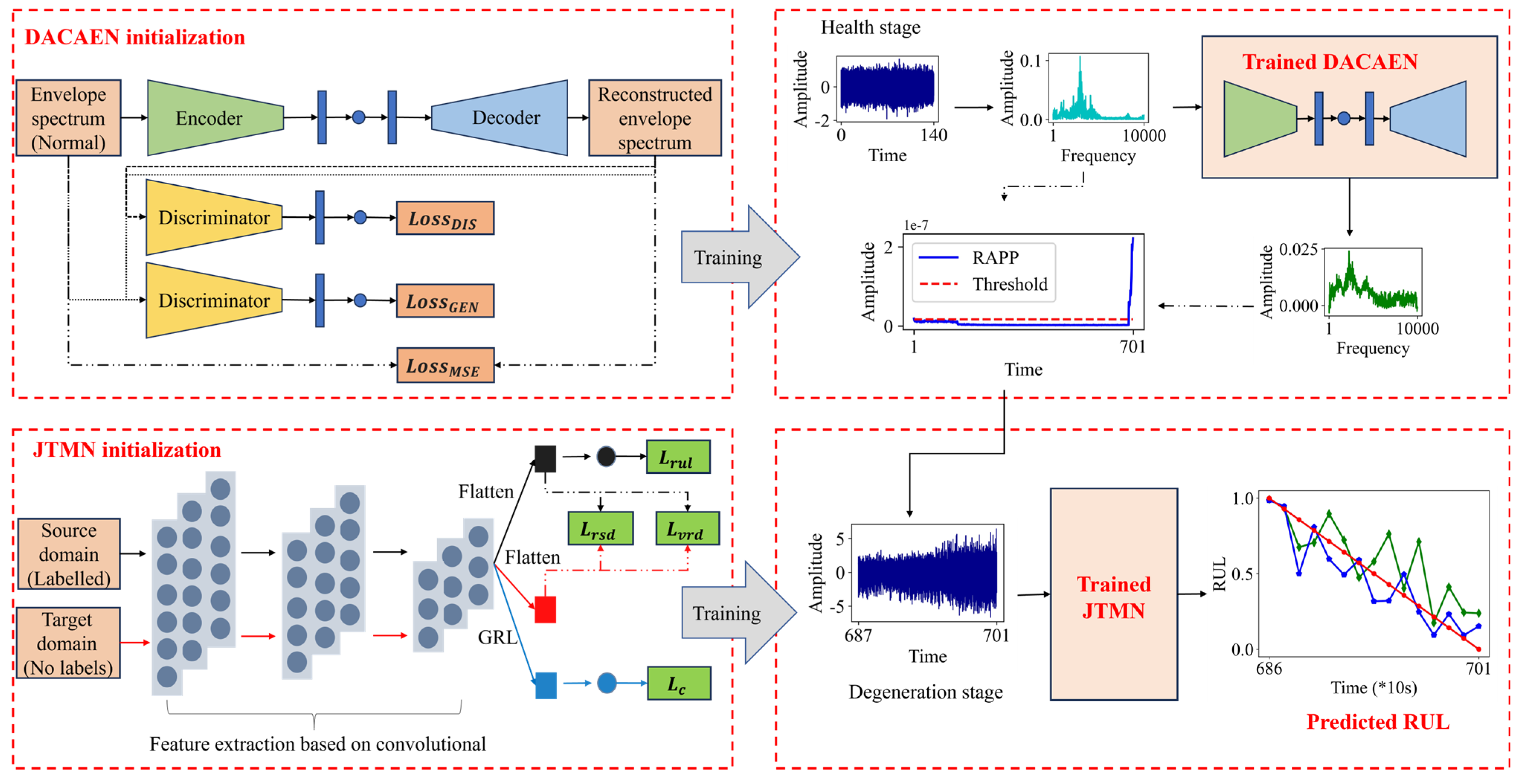
3. Proposed Cross-Working Condition RUL Prediction Method

Since the distribution discrepancies between training and testing data under cross-working conditions caused suboptimal prediction precision of rolling bearing RUL, aiming at this problem, an enhanced cross-working condition RUL prediction method via initial degradation detection-enabled joint transfer metric network is proposed and shown in Figure 1. The method includes an initial degradation detection module and a joint transfer RUL prediction module. Initial degradation detection is an essential action before RUL prediction, which is realized based on a novel RAPP health indicator created by DACAEN. Different from the reconstruction error of DCAE, RAPP compares the discrepancy between input and reconstruction of DACAEN not only in the input space, but also in the hidden spaces. The proposed joint transfer metric network focuses on feature learning of cross-working conditions, which is optimized along with regression loss and proposed joint domain adaptation loss. The former loss guarantees mapping ability from the training domain, and joint domain adaptation loss is designed for learning data distribution discrepancy reduction via VRD and the cross-domain invariant features via RSD. The proposed method can achieve higher prediction accuracy and better generalization ability than typical and advanced transfer RUL prediction methods under cross-working conditions.

3.1. RAPP-Based Initial Degradation Detection

To determine the starting point of RUL, a novel initial degradation detection method based on an RAPP health indicator is proposed. The RAPP is obtained from a novel deep adversarial convolution autoencoder network (DACAEN) and compares the discrepancy between input and reconstruction by DACAEN not only in the input space, but also in the hidden spaces, which can characterize the degradation state of rolling bearings. Combine RAPP and $3\sigma$ criteria, IDD will be completed. The details of RAPP-based initial degradation detection are described in Figure 2.

3.1.1. DACAEN Model

DACAEN is an improvement structure based on a deep convolution autoencoder network, which has been introduced as the adversarial mechanism strategy. As shown in Figure 2, DACAEN uses the vibration signal of bearings in normal stages for unsupervised model training. Then, DACAEN with high strength reconstruction ability is used for bearing condition monitoring and determine the starting point of RUL. Unlike traditional DCAE, which takes sample reconstruction loss as the optimization objective, the DACAEN model also combines the discriminant loss of the discriminator. Specifically, a fast Fourier transform (FFT) is first performed, and then the raw vibration signal obtained is fed into DACAEN to reconstruct the sample signal. At the same time, both reconstructed and original samples are input into the discriminator, so that the discriminator can distinguish the real sample and generate the sample, respectively. The structure of the encoder and discriminator in the proposed method is the same, the settings of the hyperparameters are the same, and the corresponding structure of the encoder and decoder is the same, but the corresponding convolution operation is replaced by a deconvolution operation. The specific network structure and model parameters are described in detail in the experimental section.

The amplitude of the vibration signal becomes progressively larger during the whole process of bearing operation from health to damage. When samples from the normal stage are used as training samples, it is necessary to improve identification between the degraded samples and the normal stage to realize early degradation monitoring and determine the starting point of RUL [25]. Therefore, a convolutional autoencoder network called DACAEN based on an adversarial mechanism strategy was designed in order to improve the ability of normal sample reconstruction and make the health index of the normal stage as small as possible. The input sample is denoted as $x^{in}$, and the reconstructed sample is denoted as $x^{gen}$, both of which are generated by $G\left(x^{in}\right)$. The objective function of DACAEN consists of the following three parts.

(1) Reconstruction loss ${Loss}_{MSE}$: The Euclidean distance between the real sample and the reconstructed sample, since minimizing this loss ensures that the generator produces reconstructed samples that are similar to the real sample.

$${Loss}_{MSE}={\displaystyle \frac{1}{n}}\sum _{i=1}^n\left|x_i^{gen}-x_i^{in}\right|$$

(6)

(2) Generator loss ${Loss}_{GEN}$: In order to enhance the ability of G generation and learn domain-invariant representations, the minimal-maximal game between domain discriminator and generator is leveraged. The generated samples obtained from G need to confuse D to make a wrong judgment.

$${Loss}_{GEN}={\displaystyle \frac{1}{n}}\sum _{i=1}^n\left|x_i^{gen}-x_i^{in}\right|+E_{x^{in}P{x}^{in}}\left[\mathrm{l}\mathrm{o}\mathrm{g}\left(1-D\left(G\left(x^{in}\right)\right)\right)\right]$$

(7)

where $n$ is the sample number.

(3) Discriminator loss ${Loss}_D$: Since D needs to judge the real samples $x^{in}$ from the generated samples $x^{gen}$, a fully connected layer is added to output the probability that the generated samples $x^{gen}$ are derived from the actual space.

$${Loss}_{DIS}=-\left(E_{x^{in}P{x}^{in}}\left[\mathrm{l}\mathrm{o}\mathrm{g}\left(D\left(x^{in}\right)\right)\right]+E_{x^{in}P{x}^{in}}\left[\mathrm{l}\mathrm{o}\mathrm{g}\left(1-D\left(G\left(x^{in}\right)\right)\right)\right]\right)$$

(8)

3.1.2. Construction of RAPP via DACAEN

After the training of DACAEN according to samples in the normal running stage, the reconstruction error of the normal samples has been reduced to a minimum value as far as possible, and the model lacks the reconstruction ability of the degraded samples. Therefore, the reconstruction error output by DACAEN can be used for early degradation monitoring of bearings. In the process of training the model, reconstruction loss is concerned with the Euclidean distance between the input sample and the generated sample. However, during the testing phase, differences between hidden layers were ignored. They cannot utilize the information available from the depth autoencoder projection path [26]. To address this problem, RAPP was introduced as a method for detecting novel samples using hidden space information, which provides an indirect method for calculating hidden reconstruction error by comparing the difference between the inputs and the DACAEN reconstruction, not only in the input space, but also in the hidden space [27]. Therefore, this paper combines DACAEN’s powerful sample reconstruction capability and the comprehensive information representation of RAPP based on the projection pathway of deep autoencoders. RAPP based on DACAEN is proposed to realize early degradation monitoring of bearings, as shown in Figure 2.

Given a training set $X$, let $x$ denotes the input vector from $X$ and $\widehat{x}$ represent the reconstruction of $x$. $h\left(x\right)$ denotes the hidden representations from $x,$ and $\widehat{h}\left(x\right)$ is the hidden representations from $\widehat{x}$. Let $d\left(x\right)=h\left(x\right)-\widehat{h}\left(x\right)$ and $D$ be a matrix whose $i$th row corresponds to $d\left(x_i\right)$, and let $\overline{D}$ be the column-wise centered matrix of $D$. ${\mu }_X$ denotes the column-wise mean of $D$. Then, singular value decomposition is conducted for normalization to obtain the singular values $\lambda$ and right singular vectors $V$. The traditional calculation method of the reconstruction error of Euclidean distance representation is replaced by $RAPP$, and the formula of $RAPP$ is as follows [26].

$$\overline{D}=U\lambda V^T$$

(9)

$$RAPP={‖{\left(d\left(x\right)-{\mu }_X\right)}^{T}V{\lambda }^{-1}‖}_2^2$$

(10)

3.2. JTMN-Based RUL Prediction

Traditional intelligent prediction models require that the target and training data obey independent and identical distribution. But cross-working condition situations frequently occur in real industrial environments, so the distribution discrepancies of data for training and testing often hinder promotion. While DA techniques are widely used in RUL forecasting to address this issue, RUL prediction performance needs to continue to improve to meet production needs. The performance of discrepancy metric criteria depends on the RUL prediction results using DA technology. Therefore, to build a more satisfactory intelligent prediction model aimed at cross-working condition situations, a joint domain adaptation loss is proposed to embed into a mapping regression network to build a joint transfer metric network (JTMN). The joint loss is designed to acted on the final layer of the mapping regression network combining RSD and VDR, which can weaken data distribution discrepancies and ultimately obtain cross-domain invariant features. Based on the proposed JTMN-based RUL prediction model, the RUL of rolling bearings under cross-working conditions can be predicted more precisely.

3.2.1. Joint Domain Adaptation Loss

The results demonstrated by the MMD in simulating the bearing degradation process are poor. Therefore, researchers have combined MMD with mutual information-based clustering to mitigate distribution discrepancies. Quan et al. [27] investigated the working mechanism of MMD, aiming at the risk of poor distribution alignment due to the poor discrepancy representation of the mean statistic in reproducing kernel Hilbert space (RKHS) space. A new distribution alignment metric with a new Student kernel function called variance discrepancy representation (VDR) is explored to guarantee the robustness and generalization ability of VDR [28]. Let $\mathcal{R}$ be an RKHS space. Given two data samples $X:{\left\{x_k\right\}}_{k=1}^m$ and $Y:{\left\{y_k\right\}}_{k=1}^n$ from source domain and target domain, the biased VDR statistic is the sum of two V-statistics and a sample average.

$${\mathrm{V}\mathrm{D}\mathrm{R}}_b^2\left[{\mathcal{R}}_s⨂{\mathcal{R}}_t,X,Y\right]={\displaystyle \frac{1}{m^2}}\sum _{i=1}^m\sum _{j=1}^m\tau \left(x_i,x_j\right)+{\displaystyle \frac{1}{n^2}}\sum _{i=1}^m\sum _{j=1}^m\tau \left(y_i,y_j\right)-{\displaystyle \frac{2}{mn}}\sum _{i=1}^m\sum _{j=1}^m\tau \left(x_i,y_j\right)$$

(11)

where ${\mathcal{R}}_s$ is the RKHS space from source domain and ${\mathcal{R}}_t$ is the RKHS space from target domain. $x_k$ is the $k$th sample from source domain, and $y_k$ is the $k$th sample from target domain. $m$ is the number of $X,$ and $n$ is the number of $Y$. According to ${\mu }_x={\displaystyle \frac{1}{m}}\sum _{k=1}^m\kappa \left(x_k,·\right)$,

$$\begin{gathered} \tau \left(x_i,x_j\right)={〈{\left(\kappa \left(x_i,·\right)-{\mu }_x\right)}^{⨂2},{\left(\kappa \left(x_j,·\right)-{\mu }_x\right)}^{⨂2}〉}_{{\psi }_1⨂{\psi }_2}={〈\kappa \left(x_i,·\right)-{\mu }_x,\kappa \left(x_j,·\right)-{\mu }_x〉}_{{\psi }_1⨂{\psi }_2}^2= \\ {\left\{\kappa \left(x_i,x_j\right)-{\displaystyle \frac{1}{m}}\sum _{l=1}^m\kappa \left(x_i,x_l\right)-{\displaystyle \frac{1}{m}}\sum _{k=1}^m\kappa \left(x_j,x_k\right)-{\displaystyle \frac{1}{m^2}}\sum _{l=1}^m\sum _{k=1}^m\kappa \left(x_l,x_k\right)\right\}}^2 \end{gathered}$$

(12)

Similar to $\tau \left(x_i,x_j\right)$, $\tau \left(y_i,y_j\right)$, and $\tau \left(x_i,y_j\right)$ can be respectively represented with ${\mu }_y={\displaystyle \frac{1}{n}}\sum _{l=1}^n\kappa \left(y_k,·\right)$:

$$\tau \left(y_i,y_j\right)={\left\{\kappa \left(y_i,y_j\right)-{\displaystyle \frac{1}{n}}\sum _{l=1}^n\kappa \left(y_i,y_l\right)-{\displaystyle \frac{1}{n}}\sum _{k=1}^m\kappa \left(x_j,x_k\right)-{\displaystyle \frac{1}{n^2}}\sum _{l=1}^n\sum _{k=1}^n\kappa \left(y_l,y_k\right)\right\}}^2$$

(13)

$$\tau \left(x_i,y_j\right)={\left\{\kappa \left(x_i,y_j\right)-{\displaystyle \frac{1}{n}}\sum _{l=1}^n\kappa \left(x_i,y_l\right)-{\displaystyle \frac{1}{m}}\sum _{k=1}^m\kappa \left(x_k,y_j\right)-{\displaystyle \frac{1}{nm}}\sum _{l=1}^n\sum _{k=1}^n\kappa \left(x_k,y_l\right)\right\}}^2$$

(14)

It can be seen that the kernel function $\kappa \left(x,y\right)$ is crucial for the discrepancy representation of VDR. A student kernel function $\kappa \left(x,y\right)$ is designed and introduced to solve the poor robustness for the abnormal samples and longtail distribution.

$$\kappa \left(x,y\right)={\displaystyle \frac{\Gamma \left(\frac{d+1}{2}\right)}{\sqrt{d}\Gamma \left(\frac{d}{2}\right)}}{\left(1+{\displaystyle \frac{{‖x-y‖}^2}{d}}\right)}^{-{\displaystyle \frac{d+1}{2}}}$$

(15)

where $d>0$ is the degree of freedom and $\Gamma \left(·\right)$ is the gamma function.

$$\Gamma \left(x\right)={\int }_0^{+\infty }{t}^{x-1}{e}^{-t}\mathrm{d}t,x>0$$

(16)

Although VDR is a novel distributional alignment metric that expresses variance information to enhance difference representation, it is still a metric-based approach to distributional differences. Conventional DA metrics, while effective in extracting domain-invariant representations, encounter scale misalignment issues in deep feature distributions that deteriorate regression robustness during cross-domain adaptation. Aiming at the essential characteristics of the RUL regression prediction problem, an adaptive method of the unsupervised transferable domain called representation subspace distance (RSD) is introduced to build joint domain adaptation loss for realizing accurate RUL prediction [29]. RSD belongs to a similarity measurement criterion to measure the two domains. For source domain ${\mathbf{F}}_{\mathit{s}}$ and target domain ${\mathbf{F}}_{\mathit{t}}$, the orthogonal bases of intrinsic feature subspaces are firstly calculated using the SVD algorithm:

$${\mathbf{F}}_{\mathit{s}}={\mathbf{U}}_{\mathit{s}}\mathbf{S}{{\mathbf{V}}_{\mathit{s}}}^T$$

(17)

$${\mathbf{F}}_{\mathit{t}}={\mathbf{U}}_{\mathit{t}}\mathbf{S}{{\mathbf{V}}_{\mathit{t}}}^T$$

(18)

where $\mathbf{U}$ and $\mathbf{V}$ are the left and right singular matrix, respectively; $\mathbf{U}$ and $\mathbf{V}$ are also orthogonal matrices. $\mathbf{S}=diag({\sigma }_1,{\sigma }_2,{\sigma }_3\dots )$ is a rectangular diagonal matrix with non-negative singular values decreasing in order along the diagonal.

$${{\mathbf{U}}_{\mathit{s}}}^T{\mathbf{U}}_{\mathit{t}}={\mathbf{R}}_{\mathit{s}}{\mathbf{L}}_{{\mathbf{U}}_{\mathit{s}}\leftrightarrow {\mathbf{U}}_{\mathit{t}}}{{\mathbf{R}}_{\mathit{t}}}^T$$

(19)

$${\mathbf{V}}_{\mathit{s}}{{\mathbf{V}}_{\mathit{t}}}^T={\mathbf{R}}_{\mathit{s}}{\mathbf{L}}_{{\mathit{V}}_{\mathit{s}}\leftrightarrow {\mathbf{V}}_{\mathit{t}}}{{\mathbf{R}}_{\mathit{t}}}^T$$

(20)

where ${\mathbf{L}}_{{\mathbf{U}}_{\mathit{s}}\leftrightarrow {\mathbf{U}}_{\mathit{t}}}$ denotes $diag\left(\mathrm{c}\mathrm{o}\mathrm{s}{\Theta }_{{\mathbf{U}}_{\mathit{s}}\leftrightarrow {\mathbf{U}}_{\mathit{t}}}\right)$ and ${\mathbf{L}}_{{\mathit{V}}_{\mathit{s}}\leftrightarrow {\mathbf{V}}_{\mathit{t}}}$ denotes $diag\left(\mathrm{c}\mathrm{o}\mathrm{s}{\Theta }_{{\mathit{V}}_{\mathit{s}}\leftrightarrow {\mathbf{V}}_{\mathit{t}}}\right)$. ${\Theta }_{{\mathbf{U}}_{\mathit{s}}\leftrightarrow {\mathbf{U}}_{\mathit{t}}}$ and ${\Theta }_{{\mathit{V}}_{\mathit{s}}\leftrightarrow {\mathbf{V}}_{\mathit{t}}}$ are the principal angles. The criteria for assessing similarity between the source and target domains are defined as follows:

$${Sim}_{\mathit{s},\mathit{t}}=tr({\mathbf{L}}_{{\mathbf{U}}_{\mathit{s}}\leftrightarrow {\mathbf{U}}_{\mathit{t}}}+{\mathbf{L}}_{{\mathit{V}}_{\mathit{s}}\leftrightarrow {\mathbf{V}}_{\mathit{t}}})$$

(21)

The joint domain adaptation loss, called VDR-RSD, combines the representation ability of the distribution discrepancy of VDR and the representation ability of feature manifold distribution of RSD to effectively improve the model’s ability to learn features in different domains, further enhancing cross-working condition RUL prediction performance.

3.2.2. Joint Transfer Metric Network for RUL Prediction

Traditional RUL prediction methods adopt various advanced feature extraction techniques to mine RUL-related features; however, the domain drift problem has not been solved under cross-working conditions. Fortunately, based on proposed joint domain adaptation loss, a cross-working condition RUL prediction method via a joint transfer metric network (JTMN) consisting of RUL prediction loss and joint domain adaptation loss is built. The mean square error (MSE) is used in RUL prediction loss. This will reflect the relationship between actual and predicted values. The commonly used loss function is $L_{rul}$. The joint domain adaptation loss $L_{jda}$ is a combination of $L_{vdr}$ VDR and RSD $L_{rsd}$, which operate in the high-dimensional feature layer to calculate the distribution discrepancy of representation ability and feature manifold distribution between the training domain and the testing domain. In addition, maximizing the domain classification error $L_c$ between source and target domains can further promote distribution difference alignment between the source and target domains.

In order to make JTMN have better generalization performance under a variety of working conditions, the objectives of this model improvement include loss function $L_{rul}$ from the source domain, condition generalization loss $L_{jda}$, and domain classification error $L_c$. The final loss function can be expressed as Equation (22):

$$L_{total}=L_{rul}+\mathsf{\alpha }{L}_{vdr}+\beta L_{rsd}+\gamma L_c$$

(22)

$$\gamma ={\displaystyle \frac{2}{1+\mathrm{e}\mathrm{x}\mathrm{p}(-i·e)}}-1$$

(23)

where $i$ is number of current iteration steps, $e$ is number of stop iteration steps, and $\mathsf{\alpha }$ and $\beta$ are the compromise parameters trained by back propagation. In this way, the model not only learns RUL mapping information, but also lessens distribution discrepancy. $\gamma$ is the adaptive parameters [15]. The prediction accuracy is ultimately improved under different operating conditions.

3.3. Implementation Procedures

In this paper, the frequency domain representation of the vibration signal is used as the input for DACAEN and JTMN. Combining the above two models, an enhanced RUL prediction method for rolling bearings across operating conditions is proposed. The method makes full use of historical operating conditions data in the source domain as a way to improve the generalization performance of the model in the target domain. The specific processes are as follows.

3.3.1. Data Acquisition and Signal Processing

Full-life vibration signals of rolling bearings under various operating conditions are selected, and the vibration signals are converted into a frequency domain expression by FFT to prepare for model input.

3.3.2. IDD

• The former 20% data of each bearing’s life cycle is selected to construct the training set of the input for DACAEN.
• Build the DACAEN model and initialize its parameters. The model hyperparameters are determined by grid search and cross-validation.
• Train the DACAEN model until it converges, so as to minimize the reconstruction error between the input data and the reconstructed data.
• Send the bearing life cycle data to the trained DACAEN model to build the RAPP health indicator, and combine the health threshold to realize the whole process of IDD.

3.3.3. RUL Prediction

• Set cross-domain prediction tasks according to operating conditions, build the source domain with the labeled training set and the target domain with the unlabeled training set and the target domain test set, and carry out RUL labeling processing on the source domain with the labeled training set.
• Build the JTMN model and initialize its parameters. The model hyperparameters were determined by grid search and cross-validation.
• Use the labeled source domain and unlabeled target domain as training sets to train the JTMN model until it converges, so as to minimize regression errors and distribution differences in the source domain.
• The trained JTMN is directly used for RUL prediction of the test set. The testing process can simulate an online scenario where samples taken chronologically are predicted using JTMN.
• The superior performance of the proposed method is demonstrated using evaluation indicators and analysis of the execution results.

4. Experiment Study

To demonstrate the effectiveness of the proposed RUL prediction method, several RUL prediction experiments are carried out on the bearing vibration signals. Through comparative analysis with different methods and ablation experiments, the superiority of the proposed method is verified.

4.1. Dataset Introduction

The IEEE prognostics and health management (IEEE PHM) bearing life dataset, provided by the FEMTO-ST Institute experiments, is selected as research data to carry out RUL prediction [30]. The PRONOSTIA experimental platform is shown in Figure 3.

The platform data consists of vibration data and temperature data. This experiment selects vibration data. The sampling frequency of the accelerometer is 25.6 kHz. The dataset contains three different working conditions. For example, the load is 4000 N, and the speed is 1800 rpm, under the first condition. Under the second condition, the load is 4200 N, and the speed is 1650 rpm; and the load is 5000 N and the speed is 1500 rpm under the third working condition. The specific information about the bearings is shown in

Table 1. PHM2012 dataset.

Operating Conditions	Condition_1	Condition_2	Condition_3
Datasets	Bearing1-1\Bearing1-2\Bearing1-3\Bearing1-4\Bearing1-5\Bearing1-6\Bearing1-7	Bearing2-1\Bearing2-2\Bearing2-3\Bearing2-4\Bearing2-5\Bearing2-6\Bearing2-7	Bearing3-1\Bearing3-2\Bearing3-3

, and each sample in the dataset contains data points with a length of 2560.

4.2. Model Building

The proposed method predicts RUL by two steps, as both DACAEN and JTMN need to be built. In order to adapt to the input of vibration feature representation, a 1D-convolutional feature extractor is used to construct the backbone of two networks. For the DACAEN model, the generator, made up of the encoder and the decoder, consist of three convolutional layers and three deconvolutional layers. The first convolutional layer and third deconvolutional layer use a wide convolutional kernel of size 1 × 64 with a stride of 16, while the second and third convolutional layers use small convolutional kernels of size 1 × 4 with a stride of 4. The output average pooling layer, hidden layer, and FC layer are 16, 32, and 64, respectively. The discriminator is similar to the encoder of the generator. For the JTMN model, the feature extractor is commonly used to obtained detailed degradation information about RUL. The goal of the regressor layer is to build a mapping relationship between the generated degradation information and RUL labels from the source domains. The classifier is added for division of the target domain and the training domain. The domain adaptation layer serves for joint domain adaptation loss to calculate the distribution discrepancy of representation ability and feature manifold distribution between the target domain and the training domain, which is the most important structure for the transfer ability to realize enhancement of cross-working condition RUL prediction performance. After a grid search, the parameters of $\mathsf{\alpha }$ and $\beta$ are both set as 0.1, which remain unchanged in all cross-condition prediction tasks. The Adam optimization algorithm is used in this paper, and the detailed parameters are shown in

Table 2. Detailed experimental parameters of the proposed DACAEN.

Model Name	Module Name	Network Layer	Activation Function	Stride	Size	Number	Output Size
DACAEN	Generator	Convolution layer1 + BN	Leaky relu	1 × 16	1 × 64	16	16 × 80
		Convolution layer2 + BN	Leaky relu	1 × 4	1 × 4	32	32 × 20
		Convolution layer3 + BN	Leaky relu	1 × 4	1 × 4	64	64 × 5
		Average Pooling layer	-	-	-	-	1 × 64
		Hidden layer	-	-	-	-	1 × 1
		FC layer	-	-	-	-	1 × 320
		Translation layer	-	-	-	-	64 × 5
		Deconvolution layer3 + BN	Leaky relu	1 × 4	1 × 4	32	32 × 20
		Deconvolution layer3 + BN	Leaky relu	1 × 4	1 × 4	16	16 × 80
		Reconstruction Layer3 + BN	Leaky relu	1 × 16	1 × 4	1	1 × 1280
	Discriminator	Convolution layer1 + BN	Leaky relu	1 × 16	1 × 64	16	16 × 80
		Convolution layer2 + BN	Leaky relu	1 × 4	1 × 4	32	32 × 20
		Convolution layer3 + BN	Leaky relu	1 × 4	1 × 4	64	64 × 5
		Average Pooling Layer	-				1 × 64
		FC layer	Softmax	-	1 × 1	1	1 × 1
JTMN	Feature extractor	Convolution layer1 + BN	Leaky relu	1 × 10	1 × 64	16	16 × 128
		Pooling layer	-	1 × 4	1 × 4	16	16 × 32
		Convolution layer2 + BN	Leaky relu	1 × 1	1 × 4	32	32 × 32
		Pooling layer	-	1 × 4	1 × 4	32	32 × 8
		Convolution layer3 + BN	Leaky relu	1 × 1	1 × 4	64	64 × 8
		Pooling layer	-	1 × 4	1 × 4	64	64 × 2
	Domain adaptation and regressor	Flatten layer	-		-	-	1 × 128
		FC layer 1	Sigmoid	-	-	64	1 × 64
		FC layer 2	Sigmoid	-	-	1	1 × 1
	Classifier	Gradient reversal layer	-	-	-	-	-
		FC layer 1	Softmax	-	-	2	1 × 2

.

4.3. Results and Discussion for RUL Prediction

Before implementation of RUL prediction, the bearings are first constructed for initial degradation detection, because the effect of the RUL estimation can be significantly improved with the help of initial degradation detection rather than from the start of the experiment.

4.3.1. Results and Discussion for Initial Degradation Detection

(1)

Results and Discussion

During initial degradation detection, we set the former 20% of the target bearing life data for the training of DACAEN, and the whole-life data is input into the trained model for calculating the RAPP health indicator. The results of RAPP aiming at all bearings are listed in Figure 4.

After construction of the RAPP, according to the former 20% of the target bearing life data, the health threshold of the tested bearing is obtained based on $3\sigma$ criteria. Once the RAPP exceeds the health threshold, IDD will be determined. In this paper, five consecutive RAPP values exceeding the health threshold are recorded as early degradation points. The results of IDD are listed in

Table 3. The results of IDD for IEEE PHM bearings.

Bearings	Results of IDD	Total Number of Samples	Number of Degraded Samples
Bearing 1-1	1451	2803	1352
Bearing 1-2	828	871	43
Bearing 1-3	1267	2375	1108
Bearing 1-4	1087	1428	341
Bearing 1-5	2443	2463	20
Bearing 1-6	-	2448	-
Bearing 1-7	2206	2259	53
Bearing 2-1	877	911	34
Bearing 2-2	388	797	409
Bearing 2-3	1946	1955	9
Bearing 2-4	-	751	--
Bearing 2-5	-	2311	-
Bearing 2-6	687	701	14
Bearing 2-7	225	230	5
Bearing 3-1	493	515	22
Bearing 3-2	1610	1637	27
Bearing 3-3	420	434	14

.

(2)

Ablation Study

Compared to traditional reconstruction error methods, the advantage of RAPP is attributed to the adversarial mechanism strategy of DACAEN. To demonstrate this advantage, the reconstruction ability of DACAEN and DCAE are compared. The details are shown in

Table 4. Details of the comparison.

Functions	Model Name	Ablation Name
		Adversarial Mechanism	RAPP
Reconstruction ability	DCAE	No	No
	DACAEN	Yes	No

.

Take Bearing 1-1 as an example. The reconstruction results based on DACAEN and DCAE for the frequency spectrum from two samples are shown in Figure 5. The cyan line represents the frequency spectrum in the model’s input, the green line represents the reconstructed frequency spectrum via DACAEN, and the blue represents the DCAE. It can be seen that, although DACAEN and DCAE did not completely restore the frequency spectrum at the time of input, the reconstruction of DACAEN was better than that of DCAE. This is attributed to the introduction of an adversarial mechanism strategy into DCAE.

(3)

Comparison with Popular HIs

To demonstrate the advantage of the proposed RAPP from DACAEN in constructing the HI, some popular and commonly used health indicators such as rectified average value, root mean square, root amplitude, waveform index, and average frequency are selected for comparison [31]. Take Bearing 1-1 as an example. The detailed results and the partial enlarged view are shown in Figure 6, in which the blue line represents the proposed HI, the green line represents the rectified average value, the cyan line represents the root mean square, the magenta line represents the root amplitude, the black line represents the waveform index, and the yellow line represents the average frequency.

Figure 5 shows that the proposed RAPP and average frequency display a low and stable value during the early stages of degradation. As serious performance degradation occurs in the bearings, the amplitude of HI increases significantly and exhibits a monotonic trend until the bearings fail. Although both the proposed RAPP and the average frequency effectively represent the degradation trend, it is noticed from Figure 5b that the average frequency shows more fluctuations in the healthy stages and the early stages of degradation, making it difficult to calculate the health threshold for determining abnormal points. As serious performance degradation occurs in the bearings, the amplitude of HI increases significantly and exhibits a monotonic trend until the bearings fail. However, the remaining three methods show the opposite phenomenon, with sharp burrs and large amplitude during the whole process. As an excellent indicator of degradation trends, the root mean square and root amplitude show more fluctuations in the healthy stages, making them less convenient for determining abnormal points. The waveform index suffers from poor monotonic trends and significant fluctuations throughout the process, making it difficult to accurately complete the IDD.

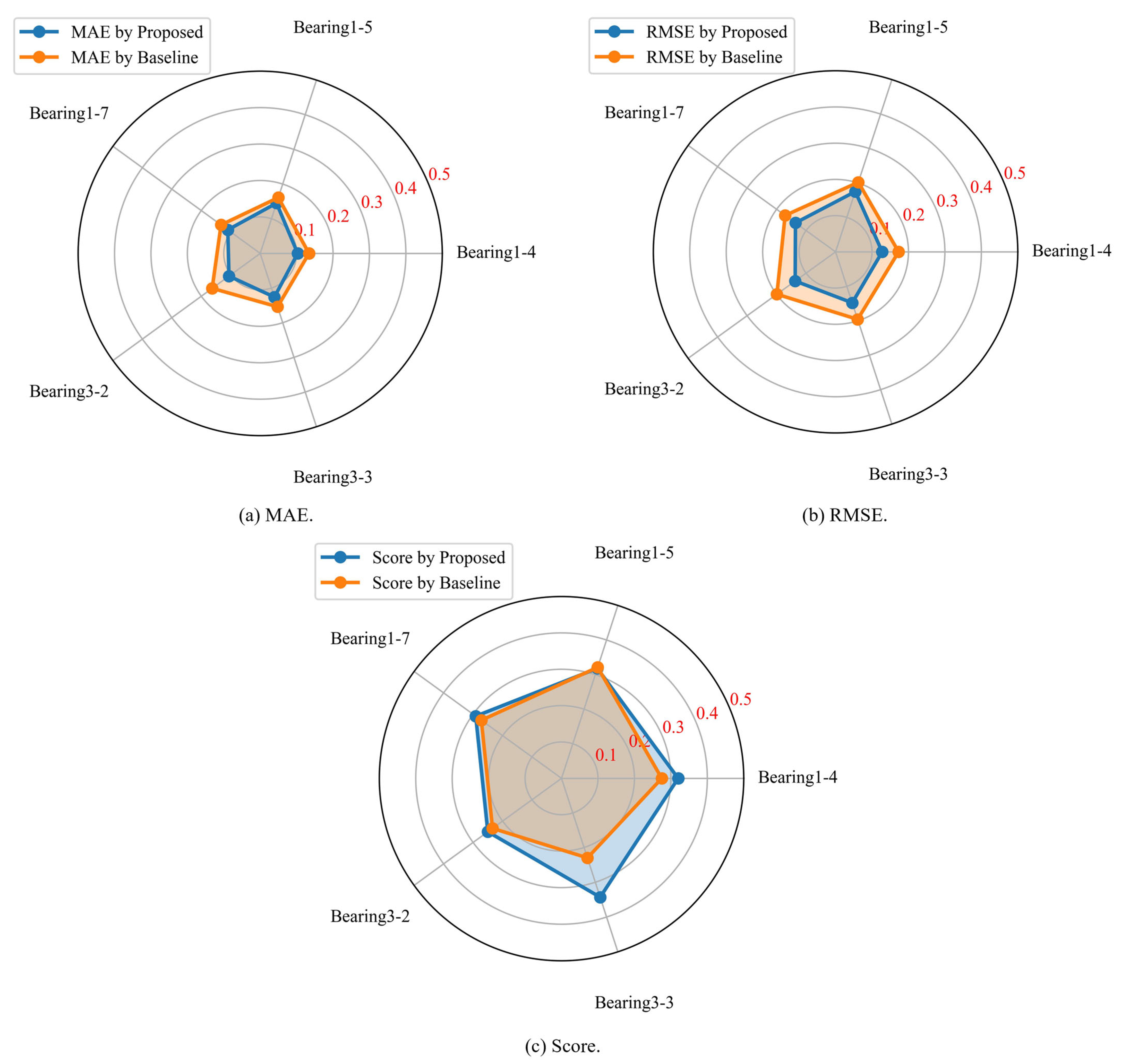
4.3.2. Results and Discussion of Cross-Working Condition RUL Prediction

After the initial degradation detection, we can obviously see that there are certain differences in the number of degradation samples among different bearings. This is because they have undergone different degradation processes. In order to achieve high-precision life prediction results, the degenerate samples with a similar total number are grouped into one class. In combination with the working conditions (three working conditions), three migration conditions were constructed, with one working condition as the source domain and the remaining two as the target domain, namely: working condition 1→2 and 3, working condition 2→1 and 3, and working condition 3→1 and 2. For the remaining bearings, Bearing 2-2 is selected as the source domain, and Bearing 1-1 is regarded as the test domain.

Table 5. Cross-working condition RUL prediction tasks.

Transfer Condition Setting	Prediction Scenario	Training Bearing		Test Bearing
		Source Domain with Label	Source Domain Without Label
1→2 and 3	Scenario A	Bearing 1-2	Bearing 2-1	Bearing 2-3/Bearing 2-6/Bearing 2-7
	Scenario B		Bearing 3-1	Bearing 3-2/Bearing 3-3
2→1 and 3	Scenario C	Bearing 2-1	Bearing 1-2	Bearing 1-4/Bearing 1-5/Bearing 1-7
	Scenario D		Bearing 3-1	Bearing 3-2/Bearing 3-3
3→1 and 2	Scenario E	Bearing 3-1	Bearing 2-1	Bearing 2-3 Bearing 2-6/Bearing 2-7
	Scenario F		Bearing 1-2	Bearing 1-4/Bearing 1-5/Bearing 1-7
2→1	Scenario G	Bearing 2-2	Bearing 1-1	Bearing 1-1

lists the specific test and RUL prediction tasks. The prediction tasks are set as follows.

(1)

Evaluation Indicators for Prediction Results

This paper is concerned with the mapping between signal features and RUL labels. The method is considered as a regression problem. Therefore, this paper uses three metrics for performance evaluation, namely mean absolute error (MAE), root mean squared error (RMSE), and Score [29]. It has been shown that the higher the score function score in the indicator, the better the model’s prediction. The smaller the MAE and RMSE, the better the model’s prediction.

(2)

Results and Discussion

According to the cross-working condition RUL prediction tasks, the trained JTMN network is used to infer the RUL of the test sample. The prediction results for all the RUL prediction tasks are shown in Figure 7, Figure 8 and Figure 9.

The blue curve represents the predicted RUL via the proposed method, the green curve represents the predicted RUL via the baseline method, and the red line represents the real RUL. It can be seen from Figure 7, Figure 8 and Figure 9 that the RUL prediction results obtained by the proposed method are most significantly improved compared with the baseline model. The blue curve fits more closely into the red line than the green curve, which shows the importance of the proposed method. Except for the abnormal decline in the Bearing 2-3 curve of scenario A, the RUL prediction showed a good downward trend in other scenarios, and the predicted curve was in good agreement with the real curve. The reasons for the abnormal RUL of Bearing 2-3 in prediction scenario A are analyzed. On the one hand, too few degenerate samples lead to prediction failure: Bearing 2-3 may not undergo a degradation process, so it does not contain degradation information, which is a sudden failure process. On the other hand, regarding the selection of training bearings, from the RUL prediction effect of Bearing 2-3 in scenario F, the proposed method can predict the RUL trend, and the proposed method is effective. These phenomena also exist in scenario A Bearing 2-7 and scenario F Bearing 2-7. On the contrary, the RUL prediction effect of scenario A Bearing 2-6 is better than that of scenario F Bearing 2-6. All these indicate that the RUL prediction effect depends on similar degradation information of the test bearing and the training bearing. In addition, it is particularly noteworthy that the predicted value is often closer to the real value in the later stage of the bearing life cycle, which is of great significance for providing accurate maintenance guidance when the bearing is close to failure.

Evaluation indicators were calculated according to the average of multiple experimental results and the MAE, RMSE, and Score of the proposed method, and the baseline values are shown in Figure 10, Figure 11 and Figure 12.

It can be seen from the figures that the quantitative results of cross-working RUL prediction using JTMN are stable and better than the baseline, which once again proves the superiority of the proposed method. Figure 13 shows the RUL prediction results of Bearing 1-1. Although this prediction method is not a cross-working condition RUL prediction, it is further proved from the RUL curve and the MAE, RMSE, and Score that the proposed method can significantly reduce the distribution difference to enhance the prediction performance compared to the baseline method.

(3)

Comparison experiment and ablation study

The JTMN framework proposed in this paper is mainly the addition of joint domain adaptation loss, called VDR-RSD, which combines the representation ability of the distribution discrepancy of VDR and the representation ability of the feature manifold distribution of RSD to effectively enhance the model’s learning of cross-domain invariant features, further enhancing cross-working condition RUL prediction performance. In order to explore the mechanisms of these losses in domain adaptive learning, the following ablation experimental studies were conducted to investigate their respective roles by gradually adding mechanisms. First, the prediction method of traditional distance measurement MMD is added based on the deep learning prediction model as the baseline. Secondly, VDR has been proved to be an improvement of MMD, and this paper uses it as a new metric instead of MMD to verify and compare its effect on RUL prediction performance. Finally, RSD was added to form joint domain adaptation loss as the main method to implement RUL prediction. Their comparative results are listed in

Table 6. Results of the ablation experiment.

Source Domain	Target Domain	Tests	Model Name
			VDR + RSD + CNN			VDR + CNN			MMD + CNN			CNN
			MAE	RMSE	Score	MAE	RMSE	Score	MAE	RMSE	Score	MAE	RMSE	Score
Bearing 1-2	Bearing 2-1	2-3	0.320	0.389	0.244	0.332	0.426	0.277	0.345	0.413	0.229	0.430	0.509	0.140
		2-6	0.082	0.105	0.316	0.115	0.132	0.354	0.088	0.115	0.347	0.121	0.156	0.384
		2-7	0.241	0.302	0.282	0.274	0.385	0.454	0.323	0.359	0.209	0.322	0.372	0.210
		AVG	0.214	0.265	0.280	0.241	0.314	0.362	0.250	0.294	0.262	0.291	0.346	0.245
	Bearing 3-1	3-2	0.115	0.150	0.373	0.081	0.105	0.375	0.111	0.131	0.312	0.159	0.183	0.173
		3-3	0.082	0.103	0.477	0.141	0.173	0.341	0.134	0.163	0.304	0.111	0.145	0.304
		AVG	0.099	0.126	0.425	0.111	0.139	0.358	0.123	0.147	0.308	0.135	0.164	0.238
Bearing 2-1	Bearing 1-2	1-4	0.103	0.128	0.320	0.137	0.166	0.186	0.115	0.140	0.245	0.134	0.173	0.275
		1-5	0.145	0.175	0.318	0.161	0.196	0.297	0.184	0.211	0.270	0.161	0.202	0.321
		1-7	0.110	0.136	0.291	0.108	0.131	0.299	0.088	0.108	0.348	0.133	0.171	0.272
		AVG	0.119	0.146	0.310	0.135	0.165	0.261	0.129	0.153	0.288	0.143	0.182	0.289
	Bearing 3-1	3-2	0.106	0.137	0.250	0.117	0.137	0.278	0.164	0.197	0.218	0.163	0.199	0.234
		3-3	0.126	0.148	0.343	0.147	0.170	0.262	0.132	0.159	0.211	0.154	0.196	0.230
		AVG	0.116	0.143	0.297	0.132	0.153	0.270	0.148	0.178	0.214	0.158	0.198	0.232
Bearing 3-1	Bearing 1-2	1-4	0.157	0.200	0.303	0.163	0.228	0.335	0.159	0.214	0.251	0.197	0.253	0.307
		1-5	0.241	0.294	0.222	0.304	0.361	0.278	0.222	0.274	0.263	0.286	0.346	0.185
		1-7	0.141	0.185	0.364	0.141	0.197	0.403	0.143	0.172	0.279	0.211	0.237	0.233
		AVG	0.180	0.226	0.297	0.203	0.262	0.339	0.175	0.220	0.264	0.231	0.279	0.242
	Bearing 2-1	2-3	0.204	0.278	0.355	0.269	0.336	0.310	0.279	0.390	0.219	0.320	0.377	0.267
		2-6	0.178	0.232	0.379	0.180	0.243	0.330	0.168	0.232	0.392	0.202	0.259	0.362
		2-7	0.132	0.154	0.269	0.155	0.254	0.497	0.208	0.259	0.324	0.241	0.317	0.334
		AVG	0.171	0.221	0.334	0.201	0.278	0.379	0.219	0.294	0.312	0.254	0.318	0.321
AVG			0.155	0.194	0.319	0.170	0.218	0.328	0.174	0.214	0.274	0.202	0.247	0.261

.

The results in Table 6 show that the RUL prediction effect of these methods gradually becomes better with the upgrade of modules. Compared with the traditional method, the proposed method shows improvement by 0.047, 0.053, and 0.058 of the MSE, RMSE, and Score. Due to a lack of understanding of the information of the target domain, the big difference in data distribution leads to poor prediction effect when using the deep learning prediction model directly. In order to make the model have the ability of cross-domain prediction, adding the traditional distance measure MMD to build the transfer learning model can achieve better prediction effect than baseline. VDR overcame the poor discrepancy representation of MMD’s mean statistic in an RKHS space. Therefore, this paper uses VDR as a new metric instead of MMD to achieve better results in most RUL prediction tasks. Nonetheless, VDR lacks the representation ability of feature manifold distribution. To effectively enhance the model’s learning of cross-domain invariant features, RSD is further combined with VDR to design joint domain adaptation loss to enhance the cross-working condition RUL, and the proposed JTMN has the expected prediction performance and the best prediction effect.

Furthermore, the metric in some domain adaptation methods, such as Wasserstein, CORrelation alignment (CORAL), and contrastive domain discrepancy (CDD), were selected to conduct comparative experiments, and the results are listed in

Table 7. Results of the comparison experiment.

Source Domain	Target Domain	Tests	Model Name
			VDR + RSD + CNN			Wasserstein + CNN			CORAL + CNN			CCD + CNN
			MAE	RMSE	Score	MAE	RMSE	Score	MAE	RMSE	Score	MAE	RMSE	Score
Bearing 1-2	Bearing 2-1	2-3	0.320	0.389	0.244	0.332	0.429	0.246	0.357	0.413	0.178	0.322	0.392	0.247
		2-6	0.082	0.105	0.316	0.122	0.145	0.226	0.087	0.108	0.342	0.112	0.138	0.329
		2-7	0.241	0.302	0.282	0.354	0.428	0.236	0.240	0.305	0.338	0.192	0.256	0.414
		AVG	0.214	0.265	0.280	0.269	0.334	0.236	0.228	0.275	0.286	0.208	0.262	0.330
	Bearing 3-1	3-2	0.115	0.150	0.373	0.103	0.130	0.365	0.111	0.137	0.317	0.168	0.232	0.314
		3-3	0.082	0.103	0.477	0.141	0.166	0.282	0.133	0.164	0.342	0.149	0.199	0.321
		AVG	0.099	0.126	0.425	0.122	0.148	0.323	0.122	0.159	0.330	0.159	0.215	0.317
Bearing 2-1	Bearing 1-2	1-4	0.103	0.128	0.320	0.101	0.124	0.278	0.335	0.386	0.356	0.123	0.153	0.242
		1-5	0.145	0.175	0.318	0.139	0.173	0.297	0.117	0.222	0.110	0.156	0.204	0.337
		1-7	0.110	0.136	0.291	0.106	0.130	0.291	0.095	0.170	0.095	0.137	0.166	0.206
		AVG	0.119	0.146	0.310	0.115	0.142	0.289	0.120	0.150	0.359	0.139	0.175	0.262
	Bearing 3-1	3-2	0.106	0.137	0.250	0.120	0.151	0.270	0.135	0.175	0.314	0.108	0.134	0.338
		3-3	0.126	0.148	0.343	0.134	0.154	0.220	0.120	0.171	0.299	0.128	0.159	0.310
		AVG	0.116	0.143	0.297	0.127	0.152	0.245	0.128	0.173	0.307	0.118	0.146	0.324
Bearing 3-1	Bearing 1-2	1-4	0.157	0.200	0.303	0.212	0.284	0.269	0.160	0.220	0.340	0.146	0.189	0.323
		1-5	0.241	0.294	0.222	0.207	0.277	0.307	0.279	0.303	0.191	0.206	0.261	0.270
		1-7	0.141	0.185	0.364	0.210	0.278	0.180	0.156	0.206	0.339	0.145	0.182	0.292
		AVG	0.180	0.226	0.297	0.209	0.280	0.252	0.199	0.243	0.290	0.166	0.211	0.295
	Bearing 2-1	2-3	0.204	0.278	0.355	0.320	0.417	0.222	0.266	0.334	0.290	0.260	0.348	0.288
		2-6	0.178	0.232	0.379	0.212	0.263	0.209	0.231	0.276	0.280	0.285	0.358	0.178
		2-7	0.132	0.154	0.269	0.281	0.311	0.213	0.234	0.281	0.208	0.227	0.282	0.273
		AVG	0.171	0.221	0.334	0.271	0.330	0.215	0.243	0.297	0.259	0.257	0.329	0.246
AVG			0.155	0.194	0.319	0.193	0.241	0.256	0.191	0.241	0.271	0.179	0.228	0.292

. The prediction MSE, RMSE, and Score are 0.179, 0.228, and 0.292 based on CCD. The prediction MSE, RMSE, and Score are 0.191, 0.241, and 0.271 based on CORAL. The prediction MSE, RMSE, and Score are 0.193, 0.241, and 0.256 based on Wasserstein. In contrast, their performances were all inferior to those based on the VDR method, and further worse than the prediction performance of the proposed method. In summary, these analysis results show that the proposed JTMN has the best prediction effect.

5. Conclusions

In this paper, an enhanced cross-working condition RUL prediction method via an initial degradation detection-enabled joint transfer metric network is proposed. This method solves the problem of insufficient RUL prediction accuracy due to differences in the distribution of the training and test data. On one hand, a novel DACAEN is built to train reconstruction ability based on healthy samples from a healthy process. The health indicator RAPP is obtained by calculating the discrepancy between the input and reconstruction of trained DACAEN, not only in the input space, but also in the hidden spaces, which is implied for the IDD, and then RUL prediction is triggered at this time. Additionally, a novel joint domain adaptation loss combined with representation subspace distance and variance discrepancy representation is designed to build a JTMN for cross-working condition RUL prediction. JTMN is enacted on the final layer of the mapping regression network to weaken data distribution discrepancies and ultimately obtain cross-domain invariant features. The experimental results from the PHM2012 bearing dataset show that the proposed method leads to superior prediction accuracy and enhanced model generalization capability compared to typical and advanced transfer RUL prediction methods under cross-over operating conditions. Its MSE, RMSE, and Score are improved by 0.047, 0.053, and 0.058, respectively.

References

1. Zou, Y.; Sun, W.; Wang, H.; Xu, T.; Wang, B. Research on Bearing Remaining Useful Life Prediction Method Based on Double Bidirectional Long Short-Term Memory. Appl. Sci. 2025, 15, 4441. [Google Scholar] [CrossRef]
2. Wu, J.; Hu, K.; Cheng, Y.; Zhu, H.; Shao, X. Temporal Multi-Resolution Hypergraph Attention Network for Remaining Useful Life Prediction of Rolling Bearings. Reliab. Eng. Syst. Saf. 2024, 247, 110123. [Google Scholar] [CrossRef]
3. Yu, J.; Shao, J.; Peng, X.; Liu, T.; Yao, Q. Remaining Useful Life of the Rolling Bearings Prediction Method Based on Transfer Learning Integrated with CNN-GRU-MHA. Appl. Sci. 2024, 14, 9039. [Google Scholar] [CrossRef]
4. Zhou, Y.; Zhang, W.; Chen, X.; Li, G. Remaining Useful Life Prediction for Machinery Using Multimodal Interactive Attention Spatial-Temporal Networks with Deep Ensembles. Expert Syst. Appl. 2025, 263, 123456. [Google Scholar] [CrossRef]
5. Song, L.Y.; Wang, H.; Zhang, J.; Liu, Z. Advancements in Bearing Remaining Useful Life Prediction Methods: A Comprehensive Review. Meas. Sci. Technol. 2024, 35, 095005. [Google Scholar] [CrossRef]
6. Yan, M.; Wang, X.; Wang, B.; Chang, M.; Muhammad, I. Bearing Remaining Useful Life Prediction Using Support Vector Machine and Hybrid Degradation Tracking Model. ISA Trans. 2020, 98, 471–482. [Google Scholar] [CrossRef]
7. Zhang, C.; Yao, X.; Zhang, J.; Tang, H. An Optimized Support Vector Regression for Prediction of Bearing Degradation. Appl. Soft Comput. 2021, 113, 107991. [Google Scholar] [CrossRef]
8. Hou, W.; Peng, Y. Adaptive Ensemble Gaussian Process Regression-Driven Degradation Prognosis with Applications to Bearing Degradation. Reliab. Eng. Syst. Saf. 2023, 239, 109543. [Google Scholar] [CrossRef]
9. Li, H.; Zhao, W.; Zhang, Y.; Zio, E. Remaining Useful Life Prediction Using Multi-Scale Deep Convolutional Neural Network. Appl. Soft Comput. 2020, 89, 106113. [Google Scholar] [CrossRef]
10. Wan, S.; Li, X.; Yin, Y.; Hong, J.; Zhang, J. Bearing Remaining Useful Life Prediction with Convolutional Long Short-Term Memory Fusion Networks. Reliab. Eng. Syst. Saf. 2022, 224, 108540. [Google Scholar] [CrossRef]
11. Zhang, B.; Li, W.; Hao, J.; Li, X.; Zhang, S. A Hybrid Algorithm for Predicting the Remaining Service Life of Hybrid Bearings Based on Bidirectional Feature Extraction. Measurement 2025, 242, 111234. [Google Scholar] [CrossRef]
12. Ding, Y.F.; Jia, M.P. Convolutional Transformer: An Enhanced Attention Mechanism Architecture for Remaining Useful Life Estimation of Bearings. IEEE Trans. Instrum. Meas. 2022, 71, 3515010. [Google Scholar] [CrossRef]
13. Wei, Y.; Wu, D. Remaining Useful Life Prediction of Bearings with Attention-Awared Graph Convolutional Network. Adv. Eng. Inform. 2023, 58, 102143. [Google Scholar] [CrossRef]
14. Hakim, M.; Omran, A.A.B.; Ahmed, A.N.; Al-Waily, M.; Abdellatif, A. A Systematic Review of Rolling Bearing Fault Diagnoses Based on Deep Learning and Transfer Learning: Taxonomy, Overview, Application, Open Challenges, Weaknesses and Recommendations. Ain Shams Eng. J. 2023, 14, 101945. [Google Scholar] [CrossRef]
15. Tian, M.; Su, X.; Chen, C.; An, W. A Novel Method for Multistage Degradation Predicting the Remaining Useful Life of Wind Turbine Generator Bearings Based on Domain Adaptation. Appl. Sci. 2023, 13, 12332. [Google Scholar] [CrossRef]
16. Lu, X.; Yao, X.; Jiang, Q.; Shen, Y.; Xu, F.; Zhu, Q. Remaining Useful Life Prediction Model of Cross-Domain Rolling Bearing via Dynamic Hybrid Domain Adaptation and Attention Contrastive Learning. Comput. Ind. 2025, 164, 104567. [Google Scholar] [CrossRef]
17. Xu, J.; Wang, Y.; Xu, L. Deep Transfer Learning Remaining Useful Life Prediction of Different Bearings. In Proceedings of the 2021 International Joint Conference on Neural Networks (IJCNN), Virtual, 18–22 July 2021; IEEE: Piscataway, NJ, USA, 2021; pp. 1–8. [Google Scholar]
18. Cheng, H.; Kong, X.; Chen, G.; Wang, Q.; Wang, R. Transferable Convolutional Neural Network Based Remaining Useful Life Prediction of Bearing Under Multiple Failure Behaviors. Measurement 2021, 168, 108286. [Google Scholar] [CrossRef]
19. Cao, Y.; Ding, Y.; Jia, M.; Tian, Z. Transfer Learning for Remaining Useful Life Prediction of Multi-Conditions Bearings Based on Bidirectional-GRU Network. Measurement 2021, 178, 109287. [Google Scholar] [CrossRef]
20. Shi, H.; Li, X.; Zhao, W.; Liu, Y. Wasserstein Distance Based Multi-Scale Adversarial Domain Adaptation Method for Remaining Useful Life Prediction. Appl. Intell. 2022, 53, 3622–3637. [Google Scholar] [CrossRef]
21. Da Costa, P.R.d.O.; Akçay, A.; Zhang, Y.; Kaymak, U. Remaining Useful Lifetime Prediction via Deep Domain Adaptation. Reliab. Eng. Syst. Saf. 2020, 195, 106682. [Google Scholar] [CrossRef]
22. Wang, Z.; Yang, B.; Li, H.; Zhang, X. Multistage Convolutional Autoencoder and BCM-LSTM Networks for RUL Prediction of Rolling Bearings. IEEE Trans. Instrum. Meas. 2023, 72, 2527713. [Google Scholar] [CrossRef]
23. Gretton, A.; Sriperumbudur, B.; Sejdinovic, D.; Fukumizu, K. Optimal Kernel Choice for Large-Scale Two-Sample Tests. In Advances in Neural Information Processing Systems 25; Curran Associates, Inc.: Red Hook, NY, USA, 2012; pp. 1205–1213. [Google Scholar]
24. Cheng, H.; Kong, X.; Yang, S.; Wang, R. Remaining Useful Life Prediction Combined Dynamic Model with Transfer Learning Under Insufficient Degradation Data. Reliab. Eng. Syst. Saf. 2023, 236, 109321. [Google Scholar] [CrossRef]
25. Qi, J.Y.; Li, C.; Chen, X.; Wang, B. Remaining Useful Life Prediction Combining Advanced Anomaly Detection and Graph Isomorphic Network. IEEE Sens. J. 2024, 24, 38365–38376. [Google Scholar] [CrossRef]
26. Shin, S.Y.; Kim, H.-J. Extended Autoencoder for Novelty Detection with Reconstruction along Projection Pathway. Appl. Sci. 2020, 10, 4497. [Google Scholar] [CrossRef]
27. González-Muñiz, A.; Díaz, I.; Cuadrado, A.A.; García, D.F. Health Indicator for Machine Condition Monitoring Built in the Latent Space of a Deep Autoencoder. Reliab. Eng. Syst. Saf. 2022, 224, 108541. [Google Scholar] [CrossRef]
28. Qian, Q.; Li, H.; Wang, J.; Zhang, Y. Variance Discrepancy Representation: A Vibration Characteristic-Guided Distribution Alignment Metric for Fault Transfer Diagnosis. Mech. Syst. Signal Process. 2024, 217, 111234. [Google Scholar] [CrossRef]
29. Qian, Q.; Li, H.; Wang, J.; Zhang, Y. Maximum Subspace Transferability Discriminant Analysis: A New Cross-Domain Similarity Measure for Wind-Turbine Fault Transfer Diagnosis. Comput. Ind. 2025, 164, 104567. [Google Scholar] [CrossRef]
30. Nectoux, P.; Gouriveau, R.; Medjaher, K.; Ramasso, E.; Morello, B.; Zerhouni, N.; Varnier, C. PRONOSTIA: An Experimental Platform for Bearings Accelerated Life Test. In Proceedings of the 2012 IEEE International Conference on Prognostics and Health Management, Spokane, WA, USA, 22–25 June 2012; IEEE: Piscataway, NJ, USA, 2012; pp. 1–8. [Google Scholar]
31. Zhang, G.; Li, X.; Chen, Y.; Li, H. Health Indicator Based on Signal Probability Distribution Measures for Machinery Condition Monitoring. Mech. Syst. Signal Process. 2023, 198, 110432. [Google Scholar] [CrossRef]
Figure 1. Structural diagram of the initial degradation detection-enabled joint transfer metric network.
Applsci 15 06401 g001
Figure 2. Network structure diagram of the proposed model.
Applsci 15 06401 g002
Figure 3. PRONOSTIA experimental platform [30].
Applsci 15 06401 g003
Figure 4. RAPP health indicator of IEEE PHM bearings.
Applsci 15 06401 g004aApplsci 15 06401 g004b
Figure 5. Reconstruction ability comparison based on DACAEN and DCAE for Bearing 1-1. (a) The first degenerated sample. (b) The eighth degenerated sample.
Applsci 15 06401 g005
Figure 6. Comparison with popular HIs for Bearing 1-1. (a) Different HIs. (b) Partial enlarged view of (a).
Applsci 15 06401 g006
Figure 7. RUL prediction results under the 1→2 and 3 transfer condition.
Applsci 15 06401 g007
Figure 8. RUL prediction results under the 2→1 and 3 transfer condition.
Applsci 15 06401 g008
Figure 9. RUL prediction results under the 3→1 and 2 transfer condition.
Applsci 15 06401 g009
Figure 10. RUL prediction results under the 1→2 and 3 transfer condition.
Applsci 15 06401 g010
Figure 11. RUL prediction results under the 2→1 and 3 transfer condition.
Applsci 15 06401 g011
Figure 12. RUL prediction results under the 3→1 and 2 transfer condition.
Applsci 15 06401 g012
Figure 13. RUL prediction results using the proposed method and baseline under the 2→1 transfer condition. (a) RUL prediction results for Bearing 1-1. (b) MAE, RMSE, and Score for Bearing 1-1.
Applsci 15 06401 g013