An Adaptive Variance Adjustment Strategy for a Static Background Error Covariance Matrix—Part I: Verification in the Lorenz-96 Model

Abstract

Accurate initial conditions are crucial for improving numerical weather prediction (NWP). Variational data assimilation relies on a static background error covariance matrix (B), yet its variance estimation is often inaccurate, affecting assimilation and forecast performance. This study introduces DRL-AST, a deep reinforcement learning-based adaptive variance rescaling strategy that dynamically adjusts the variances of B to optimize forecast skill through improved assimilation performance. By formulating variance rescaling as a Markov Decision Process and employing an actor–critic framework with Proximal Policy Optimization, DRL-AST autonomously selects spatio-temporal rescaling factors, enhancing assimilation and forecast accuracy without additional computational cost. As a new paradigm for adaptive variance tuning, DRL-AST demonstrates competitive improvements in forecast skill in experiments with the Lorenz-96 model by generating initial states that better conform to model dynamical consistency. Given its adaptability and efficiency, DRL-AST holds great potential for application in high-dimensional NWP models, where deep learning-based dimensionality reduction and reinforcement learning techniques could further enhance its feasibility and effectiveness in complex assimilation frameworks.

1. Introduction

Numerical weather prediction (NWP) serves as the cornerstone of global weather forecasting, with its accuracy highly dependent on the quality of initial conditions [1,2]. The nonlinear dynamics of atmospheric systems mean that minor initial errors can exponentially amplify, resulting in substantial deviations in short-term and extreme weather event predictions [3,4]. This sensitivity to initial conditions is a hallmark of chaotic systems that are often characterized by Lyapunov exponents, which quantify the rate at which infinitesimally close trajectories in phase space diverge [5]. A positive maximum Lyapunov exponent, the inverse of Lyapunov time, indicates exponentially growing sensitivity to perturbations, underscoring the necessity of precise initial conditions in enhancing forecast reliability. Additionally, the persistence of coherent structures in chaotic multi-attractor systems, such as the atmospheric–oceanic system, relates to the Kolmogorov–Arnold–Moser (KAM) theorem, which describes the stability of invariant tori in weakly perturbed Hamiltonian systems [6]. While the atmosphere is not a strictly Hamiltonian system, the presence of quasi-stationary regimes suggests that KAM theory may offer insights into large-scale flow predictability and the persistence of dominant weather patterns. Error accumulation becomes particularly critical in medium-range to long-range forecasts due to factors such as errors in initial conditions derived from sparse observations, limitations in physical process parameterization, inadequate representation of cross-scale interactions, constraints in vertical discretization, and inherent imperfections in theoretical modeling [7,8]. These challenges underscore the need for advanced assimilation strategies that account for the dynamical constraints imposed by chaotic system behavior. Data assimilation (DA) is a critical technique for integrating short-range predictions with observational data to improve forecasting skills. As NWP models advance toward higher resolutions, the demand for high-quality initial conditions becomes increasingly pressing, further highlighting the crucial role of data assimilation in improving forecast performance. Consequently, optimizing data assimilation systems to minimize errors due to uncertainties in initial conditions and enhance the predictive accuracy of NWP remains a fundamental scientific challenge in the field [9].

DA seeks to construct the most accurate depiction of atmospheric or oceanic states by integrating all available observations and model information. In this context, the estimation of initial conditions from sparse and noisy observations in NWP can be regarded as an ill-posed inverse problem, and DA provides a framework to mitigate the difficulties arisen from the non-uniqueness, instability, and ill conditioning of such a problem [10,11,12,13]. Among existing DA techniques, variational data assimilation (VarDA) stands out for its ability to directly incorporate unconventional observations, such as satellite and radar data, while maintaining physical and dynamical consistency with NWP models through nonlinear constraints. These attributes render VarDA indispensable for atmospheric state estimations in NWP, with three-dimensional variational assimilation (3D-Var) being particularly favored in operational rapid-update systems for its computational efficiency [14,15,16]. This method provides a correction of the model forecast by minimizing a cost function, integrating the background state, observations, and their Gaussian uncertainty statistics [17]. Operationally, the background state is derived from a short-term numerical forecast; thus, forecast errors are somehow approximate to background errors (the background state minus the ‘true’ state). However, the ‘true’ state, being empirically inaccessible, is instead represented by its statistical correlations, notably the background error covariance matrix (B-matrix), which inherently describes the probability distribution function of forecast errors. The B-matrix is a decisive parameter in the function, and it is a cornerstone of the VarDA framework, influencing information dissemination and smoothing, balancing relationships, and establishing flow-dependent properties [18]. Developing a realistic representation of the B-matrix is a primary and ongoing research focus within DA [19].

Grappling with challenges such as the elusive ‘true’ state, immense dimensionality ($n\sim {10}^7$–${10}^9$ elements) [20], and rank deficiency in the DA system, directly and explicitly constructing and operating the B-matrix are impractical [19]. In practice, a vast sample of statistical data is used to simulate background errors and then approximately estimate the B-matrix, typically consisting of model predictions or observations spanning an extended period, which are underpinned by certain and reasonable assumptions. However, since the B-matrix is typically estimated using approximate methods, it may contain substantial errors, particularly in its diagonal elements. These elements represent the variance of state variables, which directly influence the relative weighting of the background state and observations in forming the analysis state, ultimately impacting the overall performance of the DA system [21]. An overestimation of variance biases the analysis state toward observations, neglecting valuable background information, while underestimation may discard useful and crucial observational information [22].

The task of adaptively adjusting background error variances in the B-matrix through spatio-temporal scaling based on the current analysis state can be formulated as a decision-making problem. However, traditional methods, which rely on empirical settings, often yield suboptimal assimilation results due to their inability to adapt to the dynamic variability of weather systems [23,24,25]. To overcome these limitations, we introduce a new paradigm by leveraging the powerful capabilities of artificial intelligence (AI), specifically deep reinforcement learning (DRL) [26,27], through algorithms meticulously tailored to the unique demands and structural characteristics of VarDA systems. This approach enhances the flexibility and intelligence of the variance adjustment process. Specifically, we reformulate the variance adjustment task within the framework of a Markov Decision Process (MDP)—a standard model for sequential decision-making [28]—and propose an innovative method, the deep reinforcement learning adaptive spatio-temporal variance adjustment strategy (DRL-AST). In this approach, an intelligent agent—a decision-making module powered by deep neural networks—interacts with the environment, a VarDA-based framework tailored for DRL that formalizes the spatio-temporal variance adjustment process, within the VarDA analysis-prediction cycle. At each step, the agent employs a DRL policy network to map high-dimensional states to variance-scaling actions. Deep learning (DL) facilitates the state-to-action mapping by extracting spatio-temporal feature representations from complex meteorological data, enabling the policy network to generalize across varied weather conditions. The environment updates the B-matrix based on this action, performs assimilation and forecasting, and returns the next state alongside a reward reflecting assimilation performance. Ultimately, the DRL-AST iteratively optimizes cumulative rewards to derive an optimal policy network, enhancing the assimilation performance of the VarDA system. Unlike conventional methods, DRL-AST leverages adaptive spatio-temporal adjustments to generate initial states with improved dynamic consistency relative to the numerical model. This approach improves assimilation performance, thereby substantially boosting the predictive accuracy of the numerical model.

The main contributions in this study are as follows:

• Proposing a spatio-temporally adaptive variance rescaling strategy based on deep reinforcement learning: this study develops the DRL-AST method, which enables the spatio-temporal adaptation of the variance of the static B-matrix without incurring additional computational costs. This approach improves the adaptability of data assimilation, thereby enhancing analysis quality and forecast skill.
• Improving performance over long-term assimilation periods: by adaptively rescaling the variance of the B-matrix through spatio-temporal optimization, DRL-AST demonstrates competitive robustness and accuracy in long-term assimilation cycles by consistently reducing analysis errors under varying observational noise levels, while maintaining high computational efficiency.
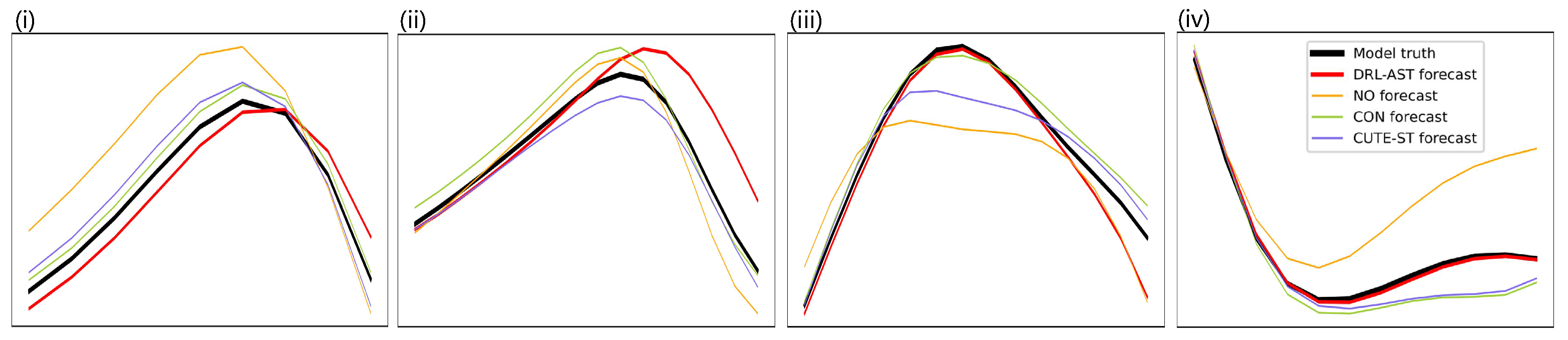
• Improving forecast skill and stability (validated in the Lorenz-96 model): leveraging a gated recurrent unit (GRU) module to learn historical assimilation states, DRL-AST ensures that the analysis state better aligns with the forecast model’s dynamical evolution. In the Lorenz-96 model, the experimental results demonstrate that DRL-AST effectively delays error growth compared to other methods, thereby improving the accuracy and stability of forecasts.

The structure of this study is as follows. Section 2 offers a comprehensive overview of related research. Section 3 outlines the necessary preliminaries. In Section 4, we introduce a spatio-temporal adaptive rescaling factor selection strategy for the variance of the B-matrix, leveraging deep reinforcement learning. Section 5 presents the experimental setup, results, and analysis. Section 6 discusses the limitations of the proposed approach and potential directions for future research. Finally, Section 7 concludes this study.

2. Related Studies

This section reviews existing approaches for variance adjustment in VarDA systems, highlighting their methodological advancements and inherent limitations. It then examines the role of deep learning (DL) and reinforcement learning (RL) in Earth science and data assimilation.

2.1. Traditional Methods for Variance Adjustment in VarDA Systems

2.1.1. Empirical Variance Rescaling

Derber and Bouttier (1999) introduced a fixed rescaling factor (0.81) to B of the European Centre for Medium-Range Weather Forecasts (ECMWF) assimilation system, mitigating variance overestimation inherent in the National Meteorological Center (NMC) method [29]. Although this adjustment improved medium-latitude forecasts, its globally uniform application failed to capture spatial and temporal variations, particularly in tropical regions where weaker geostrophic balance necessitates localized corrections.

To address the variance underestimation of Ensemble of Data Assimilation (EDA)-based B, Bonavita et al. (2012) applied a global factor of approximately 2 in ECMWF’s 4D-Var system [23]. Despite improving deterministic analysis quality, the lack of flow dependency limited its ability to account for regional and seasonal variations in background error characteristics. Similarly, Bormann et al. (2016) examined the role of observation error covariance (R) adjustments in IASI data assimilation, demonstrating that when inter-channel error correlations were ignored, an inflation factor ranging between 2.5 and 3 improved assimilation performances, while explicitly modeling these correlations reduced the optimal factor to 1.75 [24]. These findings underscore that variance tuning in variational assimilation must consider the interdependence between background and observation error specifications in order to achieve optimal performance.

Jung et al. (2024) scaled the background error standard deviations in B by a factor of 1/3 to match the 6 h assimilation cycle in JEDI-MPAS 3D-Var, where B was statistically derived from 366 forecast differences between 48 h and 24 h lead times using NCEP GFS data [25]. They also halved the diagnosed horizontal correlation lengths for the stream function and unbalanced velocity potential, correcting discrepancies between training-derived correlations and the Background Error on Unstructured Mesh Package (BUMP) assumptions. These adjustments increased velocity variance by a factor of 4, aligning better with training data and improving assimilation performance. Their results underscore the need for adaptive variance rescaling in enhancing the DA system’s accuracy.

2.1.2. Adaptive Variance Updating

Desroziers et al. (2005) developed a diagnostic-based variance tuning method, iteratively adjusting B and R based on statistical consistency relations in an observation space [30]. Applied to the French ARPEGE 4D-Var system, this method identified the systematic overestimation of background and observation errors, improving variance estimates and capturing observation error correlations. However, its effectiveness hinges on the availability of high-density, high-quality observations and assumes independence between background and observation errors, limiting robustness in data-sparse regions. Furthermore, the method lacks flow-dependent and temporally adaptive covariance adjustments, restricting its operational applicability.

To enhance adaptability, Cheng et al. (2019) proposed two iterative methods, Covariance Updating iTerativE (CUTE) and Partially Updating Best Linear Unbiased Estimator (PUB) [31]. These approaches iteratively refine B by incorporating evolving background-observation error covariances, introducing a scaling factor ($\alpha$) to regulate variance trace and prevent excessive reduction over iterations. CUTE directly updates B based on background-observation error covariance, while PUB extends the assimilation space by jointly optimizing B and R. Despite improving error correlation estimation and assimilation accuracy, these methods contradict the independence assumption of B in variational assimilation, potentially resulting in non-convergence. PUB incurs higher computational costs, and its optimization impact on assimilation performance is less pronounced than that of CUTE. Both methods rely on empirically tuned scaling factors, limiting their full adaptability in high-dimensional applications.

Hybrid data assimilation methods offer an alternative by combining ensemble-derived and static background error covariances, introducing flow dependency while maintaining statistical robustness [17,32]. By weighting these components, hybrid approaches indirectly adapt background error variances as ensemble covariances naturally evolve over time. However, these methods demand substantial computational resources due to the need for ensemble forecasts. Additionally, Bonavita et al. (2012) demonstrated that even when using ensemble-derived covariances, additional variance rescaling is often necessary to correct systematic underestimation [23]. The reliance on the empirical tuning of weight coefficients between ensemble and static covariances further limits adaptability, presenting operational challenges in high-dimensional systems.

2.2. Deep Learning and Reinforcement Learning in Earth Science and Data Assimilation

2.2.1. Deep Learning for Feature Extraction in Earth System Science

In VarDA, accurately tuning the variances of the B-matrix remains a persistent challenge, with traditional methods often sacrificing performance or computational efficiency. Recent advancements in artificial intelligence (AI) have introduced transformative solutions to Earth system science under the ‘AI for Science’ (AI4S) paradigm [33,34]. Deep learning (DL) has notably revolutionized weather forecasting through large weather models (LWMs) such as GraphCast [35], NowcastNet [36], and Pangu [37]. These models exploit neural networks to extract intricate features from high-dimensional geophysical data, substantially enhancing prediction accuracy and computational speed.

Beyond forecasting, DL has enriched various facets of DA, including model error correction, dynamical system identification, and reduced-order surrogate modeling [38]. For instance, DL techniques such as autoencoders support reduced-order modeling by compressing high-dimensional systems, while neural networks aid in identifying hidden dynamics and correcting model biases. DL has also been utilized for specifying the R-matrix in DA. Cheng et al. (2022) employed long short-term memory (LSTM) networks to predict R from observational sequences, benefiting from LSTM’s capability to handle temporal dependencies [39]. This approach notably enhances dynamic R estimation within DA frameworks. However, such methods rely on the availability of a known R-matrix as a training target—a condition that does not hold for the B-matrix, rendering direct adaptation infeasible. This underscores the necessity for alternative AI-driven approaches for background error covariance adjustment.

2.2.2. Reinforcement Learning for Data Assimilation and Forecasting

Reinforcement learning (RL) is an AI approach designed to optimize decision-making by enabling agents to interact with their environment and learn policies that maximize cumulative rewards [26]. Specifically, RL agents refine their strategies through trial and error, continuously adapting to dynamic conditions in order to achieve optimal outcomes. In Earth science and DA, RL applications remain in their early stages. However, emerging research suggests that integrating RL with DL could provide effective solutions for tackling complex decision-making challenges in nonlinear systems.

Unlike the ensemble Kalman filter (EnKF), which relies on Gaussian assumptions and linear updates, Hammoud et al. (2024) proposed an RL-based DA approach [40]. In their framework, an RL agent is employed within each assimilation window to generate a correction vector based on the current model state and observational innovation. This correction is added to the background forecast to update the state estimation of chaotic dynamical systems. The proposed method exhibits advantages in handling nonlinear and non-Gaussian systems, improving forecast accuracy [41]. Experiments on Lorenz-63 and Lorenz-96 models demonstrated superior performance over EnKF, particularly under high noise levels. However, because the correction vector shares the same dimensionality as the numerical model state, scalability to high-dimensional systems may impose substantial computational burdens. Furthermore, the correction strategy may have overlooked physical consistency among state variables, which could potentially introduce spurious errors. Similarly, Jeung et al. (2023) introduced an RL-based automatic assimilation model (SWMM-RL) to improve the accuracy of urban stormwater runoff and water quality simulations [42]. In this approach, during each storm event, an RL agent outputs optimized input parameters for the Storm Water Management Model (SWMM) based on environmental states, with the goal of minimizing prediction errors. This framework can be viewed as an event-driven, offline-trained, data-driven parameter calibration strategy that enhances the adaptability of the model to varying environmental conditions. SWMM-RL substantially improves the prediction of runoff volumes and pollutant loads—especially under extreme rainfall scenarios—compared to traditional fixed-parameter approaches. Nevertheless, the model exhibits instability in low-rainfall scenarios, and its generalization capability requires further validation across broader and more complex conditions. However, applying a single RL agent to the entire study area may overlook localized watershed variations.

Beyond direct DA applications, RL has demonstrated its potential in handling nonlinear forecasting problems in Earth system sciences by framing predictive tasks as sequential decision-making processes, enabling adaptive model refinement and improved uncertainty estimation in complex, dynamic environments. Zhao et al. (2024) proposed a dynamic ensemble forecasting method (DDPG-WRF-TBL) that integrates NWP, deep deterministic policy gradient (DDPG), and error sequence correction (TCN-BiLSTM) to enhance multi-step wind speed forecasting [43]. The key innovation lies in dynamically adjusting ensemble weights to avoid the low-performing member and optimizing forecast accuracy by prioritizing reliable simulations. However, the method’s effectiveness remains dependent on the quality of NWP outputs. Wu et al. (2025) developed an RL-based ensemble forecasting framework (RL-EFF) for renewable energy prediction, employing a deep Q-network (DQN) to dynamically select the most suitable base models based on meteorological conditions [44]. This approach overcomes the limitations of traditional ensemble methods that rely on fixed model combinations, thereby improving adaptability and predictive accuracy. Despite its advantages, the discrete action space of RL-EFF may limit its ability to fully integrate base model outputs.

3. Preliminaries

3.1. Variational Formulation

Variational data assimilation (VarDA) estimates the optimal analysis state ${\mathbf{x}}^a$ by minimizing the cost function:

$$\begin{array}{c}\hfill J_{cost}\left(\mathbf{x}\right)={\displaystyle \frac{1}{2}}{(\mathbf{x}-{\mathbf{x}}^b)}^T{\mathbf{B}}^{-1}(\mathbf{x}-{\mathbf{x}}^b)+{\displaystyle \frac{1}{2}}{({\mathbf{y}}^o-\mathcal{H}\left(\mathbf{x}\right))}^T{\mathbf{R}}^{-1}({\mathbf{y}}^o-\mathcal{H}\left(\mathbf{x}\right)).\end{array}$$

(1)

The nonlinear observation operator $\mathcal{H}$ is locally linearized around ${\mathbf{x}}^b$ as follows:

$$\begin{array}{c}\hfill \mathcal{H}\left(\mathbf{x}\right)\approx \mathcal{H}\left({\mathbf{x}}^b\right)+\mathbf{H}(\mathbf{x}-{\mathbf{x}}^b),\end{array}$$

(2)

where

$$\begin{array}{c}\hfill \mathbf{H}={\displaystyle \frac{\partial \mathcal{H}\left(\mathbf{x}\right)}{\partial \mathbf{x}}}{|}_{\mathbf{x}={\mathbf{x}}^b}.\end{array}$$

(3)

The observation discrepancy expands as follows:

$$\begin{array}{c}\hfill {\mathbf{y}}^o-\mathcal{H}\left(\mathbf{x}\right)={\mathbf{y}}^o-\mathcal{H}\left({\mathbf{x}}^b\right)-\mathbf{H}(\mathbf{x}-{\mathbf{x}}^b),\end{array}$$

(4)

Thus, the gradient of the cost function is expressed as follows:

$$\begin{array}{c}\hfill \nabla J_{cost}\left(\mathbf{x}\right)={\mathbf{B}}^{-1}(\mathbf{x}-{\mathbf{x}}^b)-{\mathbf{H}}^T{\mathbf{R}}^{-1}({\mathbf{y}}^o-\mathcal{H}\left({\mathbf{x}}^b\right)-\mathbf{H}(\mathbf{x}-{\mathbf{x}}^b)).\end{array}$$

(5)

Setting $\nabla J_{cost}\left(\mathbf{x}\right)=0$ results in the following analysis update:

$$\begin{array}{c}\hfill {\mathbf{x}}^a={\mathbf{x}}^b+{[{\mathbf{B}}^{-1}+{\mathbf{H}}^T{\mathbf{R}}^{-1}\mathbf{H}]}^{-1}{\mathbf{H}}^T{\mathbf{R}}^{-1}({\mathbf{y}}^o-\mathcal{H}\left({\mathbf{x}}^b\right)).\end{array}$$

(6)

Below

Table 1. Summary of mathematical notations used in Section 3.

Symbol	Description	Definition
Variational Data Assimilation (VarDA) (notations used in Section 3.1)
$\mathbf{x}$	State vector	Model variables (e.g., temperature, winds, pressure)
${\mathbf{x}}^b$	Background state	Prior estimate of the state
${\mathbf{x}}^a$	Analysis state	Optimized estimate after data assimilation
${\mathbf{x}}^t$	True state	Theoretical true state of the atmosphere, unknown in practice
${\mathbf{y}}^o$	Observations	Atmospheric and multi-modal observational data
$\mathcal{H}$	Observation operator	Map from model space to observation space
$\mathbf{H}$	Tangent linear of the observation operator	$\mathbf{H}={\displaystyle \frac{\partial \mathcal{H}}{\partial \mathbf{x}}}$
$\mathbf{B}$	Background error covariance matrix	Represents uncertainty in background state
$\mathbf{R}$	Observation error covariance matrix	Represents uncertainty in observations
$J_{cost}\left(\mathbf{x}\right)$	Cost function	Minimization objective in variational data assimilation
Background Error Covariance Matrix (notations used in Section 3.2)
$\epsilon$	Background error vector	Difference between background and true state
${\sigma }_i^2$	Variance	Diagonal element of $\mathbf{B}$, representing the background error variance of the i-th state variable, $i=1,2,\dots ,n$
${\rho }_{mn}$	Correlation coefficient	${\rho }_{mn}={\displaystyle \frac{\overline{{\epsilon }_m{\epsilon }_n}}{{\sigma }_m{\sigma }_n}},m\ne n$; measures linear dependence between different variables
$\mathbf{C}$	Correlation matrix	Matrix composed of ${\rho }_{mn}$
$\mathbf{D}$	Diagonal matrix	Contains the background error standard deviations
Deep Reinforcement Learning (notations used in Section 3.3)
$\mathcal{S}$	State space	Set of all possible states in the RL environment
$\mathcal{A}$	Action space	Set of all possible actions an agent can take
$P\left(s_{t+1}\right|s_t,a_t)$	State transition function	Conditional probability density function of transitioning to $s_{t+1}$ given $s_t$ and $a_t$, where t denotes timestep
$R(s_t,a_t)$	Reward function	A scalar reward received after taking action $a_t$ in state $s_t$, quantifying the immediate impact of the action
$\gamma$	Discount factor	A scalar ranging between 0 and 1 that discounts long-term rewards
${\pi }_{\theta }$	Policy	A stochastic policy parameterized by $\theta$ that maps each state to a distribution over actions
$G_t$	Return at t	Discounted sum of future rewards from time t
$\tau$	Trajectory	A sequence of states and actions: $\tau =(s_0,a_0,s_1,a_1,\dots ,s_T,a_T)$, where T denotes the total time

is the summary of mathematical notations used in Section 3.

3.2. Background Error Covariance Matrix

When $\mathbb{E}\left[\epsilon \right]=\mathbf{0}$, indicating that the expectation of each error component is zero, $\mathbf{B}$ can be expressed as the expectation of the outer product of error vector $\epsilon$:

$$\begin{array}{c}\hfill \mathbf{B}=\mathbb{E}\left[(\epsilon -\mathbb{E}\left[\epsilon \right]){(\epsilon -\mathbb{E}\left[\epsilon \right])}^T\right]=\mathbb{E}\left[\epsilon {\epsilon }^T\right]=\left[\begin{array}{cccc}\overline{{\epsilon }_1{\epsilon }_1}& \overline{{\epsilon }_1{\epsilon }_2}& \dots & \overline{{\epsilon }_1{\epsilon }_n}\\ \overline{{\epsilon }_2{\epsilon }_1}& \overline{{\epsilon }_2{\epsilon }_2}& \dots & \overline{{\epsilon }_2{\epsilon }_n}\\ ⋮& ⋮& & ⋮\\ \overline{{\epsilon }_n{\epsilon }_1}& \overline{{\epsilon }_n{\epsilon }_2}& \dots & \overline{{\epsilon }_n{\epsilon }_n}\end{array}\right].\end{array}$$

(7)

where the overline denotes the expectation. $\mathbf{B}$ is symmetric and positive-definite, where diagonal elements correspond to the variance of each error component:

$$\begin{array}{c}\hfill \overline{{\epsilon }_i{\epsilon }_i}={\sigma }_i^2.\end{array}$$

(8)

To obtain a normalized form, each element of $\mathbf{B}$ is divided by the product of the corresponding standard deviations, yielding correlation matrix $\mathbf{C}$:

$$\begin{array}{c}\hfill \mathbf{C}=\left[\begin{array}{cccc}1& {\rho }_{12}& \dots & {\rho }_{1n}\\ {\rho }_{12}& 1& \dots & {\rho }_{2n}\\ ⋮& ⋮& & ⋮\\ {\rho }_{1n}& {\rho }_{2n}& \dots & 1\end{array}\right].\end{array}$$

(9)

If $\mathbf{D}=\left[\begin{array}{cccc}{\sigma }_1& 0& \dots & 0\\ 0& {\sigma }_2& \dots & 0\\ ⋮& ⋮& & ⋮\\ 0& 0& \dots & {\sigma }_n\end{array}\right]$, then $\mathbf{B}$ can be reconstructed as follows:

$$\begin{array}{c}\hfill \mathbf{B}=\mathbf{D}\mathbf{C}\mathbf{D}.\end{array}$$

(10)

If a single observation of an element in $\mathbf{x}$ is introduced in Equation (6), assuming that it coincides with an analysis grid point corresponding to the i-th element of the state vector, $\mathbf{H}$ simplifies to a row vector with all elements set to zero except for the i-th entry, which is equal to one. Under this assumption, the observation and observation error covariance are reduced to scalars, i.e., ${\mathbf{y}}^o=y^o$ and $\mathbf{R}=R_{ii}$. Consequently, the analysis increment for the i-th element follows from Equation (6):

$$\begin{array}{c}\hfill x_i^a-x_i^b=B_{ii}{\displaystyle \frac{y^o-x_i^b}{B_{ii}+R_{ii}}}.\end{array}$$

(11)

where $B_{ii}={\sigma }_i^2$, representing the variance of the background error at the i-th state variable. The relative magnitudes of $B_{ii}$ and $R_{ii}$ govern the assimilation outcome—if $R_{ii}\ll {\sigma }_i^2$, then $x_i^a\to y^o$—indicating that the observation is dominant; conversely, if ${\sigma }_i^2\ll R_{ii}$, then $x_i^a\to x_i^b$, which indicates that the analysis remains closer to the background state. This underscores the critical role of the background error variances, which balances background and observational contributions according to their respective uncertainties.

Since the true state ${\mathbf{x}}^t$ is unobservable in practical scenarios, various methodologies were developed to estimate the background error covariance matrix $\mathbf{B}$ using surrogate background error samples [19]. Among these, the NMC method [29] is widely employed by major forecasting centers due to its practical advantages. This approach estimates $\mathbf{B}$ by computing the statistical difference between pairs of model forecasts initialized at different lead times but that are valid at the same forecast time. Specifically, the covariance is approximated as follows:

$$\begin{array}{c}\hfill \mathbf{B}\approx {\displaystyle \frac{1}{2}}〈({\mathbf{x}}^{48}-{\mathbf{x}}^{24}){({\mathbf{x}}^{48}-{\mathbf{x}}^{24})}^T〉,\end{array}$$

(12)

where ${\mathbf{x}}^{48}$ and ${\mathbf{x}}^{24}$ denote 48 h and 24 h forecasts, respectively, carrying out verifications at the same forecast time.

3.3. Deep Reinforcement Learning

Reinforcement learning (RL) aims to learn an optimal decision-making strategy through trial and error. Formally, RL is formulated as a Markov Decision Process (MDP), defined by the tuple $\langle \mathcal{S},\mathcal{A},P,R,\gamma \rangle$ [26,28]. At each timestep t, the agent observes the current state $s_t\in \mathcal{S}$, selects an action $a_t\in \mathcal{A}$ according to a policy $\pi$, and receives a reward $R(s_t,a_t)$. The environment then transitions to $s_{t+1}$ based on the transition function $P(s_{t+1}\mid s_t,a_t)$, which is the conditional probability density function describing the probability density of transitioning to the next state $s_{t+1}$ given the current state $s_t$ and the action $a_t$. The objective is to derive an optimal policy that maximizes the expected cumulative return:

$$\begin{array}{c}\hfill G_t=\sum _{t=0}^{\infty }{\gamma }^{t}R(s_t,a_t),\end{array}$$

(13)

where $\gamma \in [0,1)$ is the discount factor weighting long-term rewards.

Deep reinforcement learning (DRL) extends RL by leveraging deep neural networks to approximate value functions or directly parameterizing the policy. This enables learning in high-dimensional state–action spaces, facilitating applications in complex domains such as autonomous systems [45], strategic gameplay [46], and financial modeling [47].

4. Approach

4.1. Benchmark for VarDA System

The Lorenz-96 model, a nonlinear system capable of exhibiting chaotic behavior, serves as a simplified alternative to complex numerical weather prediction models. Its reduced computational demands facilitate the exploration of diverse atmospheric scenarios, effectively capturing essential chaotic dynamics of the atmosphere. Consequently, the Lorenz-96 model is widely used in data assimilation research [48,49,50]. The governing equations are as follows:

$$\begin{array}{c}\hfill {\displaystyle \frac{d{X}_j}{dt}}=\left(X_{j+1}-X_{j-2}\right)X_{j-1}-X_j+F\end{array}$$

(14)

where $j=1,2,\dots ,J$. Here, the model parameters are chosen to be identical to those reported by the authors of [48]. Namely, $J=40$ denotes the scalar state variables on 40 equally spaced grid points around a latitude circle. The forcing term $F=8.0$ and a fourth-order Runge–Kutta scheme (RK4) with a time step of $dt=0.05$ (counting as 6 h) are used for solving the equations numerically.

The ‘true’ sequence of weather is represented by a specific time-dependent solution of Equation (14), ideally showing the real underlying dynamics. Firstly, the initial state of the Lorenz-96 model is set as follows:

$$\begin{array}{c}\hfill X_j=\left\{\begin{array}{cc}F\hfill & \mathrm{if}j\ne 20\hfill \\ 1.001F\hfill & \mathrm{if}j=20\hfill \end{array}\right.\end{array}$$

(15)

Subsequently, the model is integrated forward for 360 steps (equivalent to 90 days) to eliminate transient behavior, consistent with Lorenz’s 1998 study [48]. After this initialization period, the model is continuously integrated forward for an additional 5 years (7200 steps) to generate the ‘true’ sequences of meteorological quantities. If necessary, the integration can be extended for a longer period to suit specific research requirements.

4.2. DRL-Based Formulation for the VarDA System

In this study, we reformulate the traditional VarDA system into an interactive environment compatible with DRL, allowing an agent to learn a policy for adaptively scaling the spatio-temporal variances of the $\mathbf{B}$-matrix. This customized environment, referred to as the spatio-temporal variance-weighting environment for the VarDA system (abbreviated as VarDA W-ST), is illustrated in Figure 1, where the DA process is marked by circled steps ①–⑦, and the agent–environment interaction is indicated by steps (1)–(3).

The system first estimates the static background error covariance matrix, ${\mathbf{B}}_{\mathrm{NMC}}$, using the NMC method [29], which analyzes 500 forecast difference pairs following a 50-day spin-up period (①). Starting from the initial condition, the Lorenz-96 model is integrated forward for 6 h to obtain the background state at time t, denoted as ${\mathbf{x}}_t^b$ (②), which serves as the prior for the assimilation step. The first forecast is initialized with the predefined state from Equation (15), while subsequent forecasts use the analysis ${\mathbf{x}}_t^a$ from the previous cycle as the initial condition. Observations ${\mathbf{y}}_t^o$ are assimilated every 6 h by incorporating the innovation ${\mathbf{d}}_t={\mathbf{y}}^o-\mathcal{H}\left({\mathbf{x}}_t^b\right)$ into the VarDA system to correct the background state (③). To enable spatially adaptive variance scaling and improve numerical stability, ${\mathbf{B}}_{\mathrm{NMC}}$ is first normalized globally to yield ${\mathbf{B}}_{\mathrm{norm}}$ (④), which is then partitioned into ${\mathbf{B}}_{\mathrm{norm}}^{\left(ck\right)}$ for each spatial chunk $ck=1,2,\dots ,CK$, where $CK$ is the total number of chunks. Here, ${\mathbf{B}}_{\mathrm{norm}}^{\left(ck\right)}$ represents the portion of the globally normalized ${\mathbf{B}}_{\mathrm{norm}}$ corresponding to the $ck$-th spatial chunk. Such normalization is widely adopted in the VarDA system to eliminate spatially inhomogeneous variances, improve the conditioning of $\mathbf{B}$, and ensure consistent variance tuning across variables and scales, thereby facilitating chunk-wise modulation strategies [19]. In step (1), the current analysis state $s_t={\mathbf{x}}_t^a$ is passed to the agent, which outputs a chunk-wise scaling vector $\mathbf{W}=[w_1,\dots ,w_{CK}]$ (step (2)). This action is then applied to ${\mathbf{B}}_{\mathrm{norm}}^{\left(ck\right)}$ to produce the rescaled matrix ${\mathbf{B}}_{\mathbf{W}}$, where ${\mathbf{B}}_{\mathbf{W}}^{\left(ck\right)}=w_{ck}·{\mathbf{B}}_{\mathrm{norm}}^{\left(ck\right)}$ for each chunk $ck=1,2,\dots ,CK$, and all chunk-wise scalings are performed simultaneously to form the complete ${\mathbf{B}}_{\mathbf{W}}$ (⑤, step (3)). Initially, the scaling vector is randomly sampled. In later cycles, it is adaptively generated by the policy network trained using DRL-AST (see Section 4.4). The analysis state ${\mathbf{x}}_t^a$ is then computed by the VarDA system (⑥) based on the background state, innovation, and the rescaled covariance matrix ${\mathbf{B}}_{\mathbf{W}}$. This updated analysis ${\mathbf{x}}_t^a$ is used as the initial condition for the next forecast (⑦), thereby continuing the sequential forecast-assimilation process.

Building on this structure, we formalize the process of spatio-temporal variance rescaling—based on the static $\mathbf{B}$-matrix estimated via the NMC method—as an MDP defined by the following components:

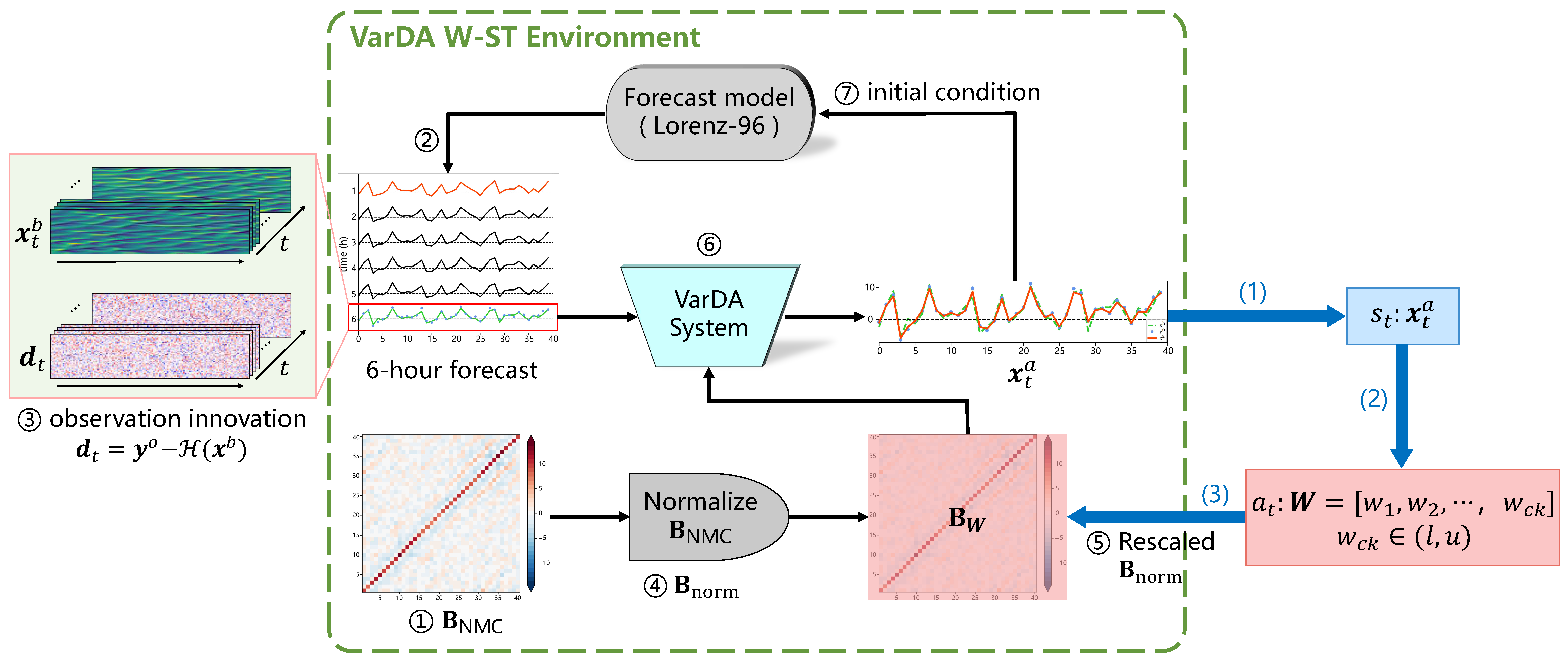
• State$s_t$ represents the analysis state ${\mathbf{x}}_t^a$ produced by the VarDA system at time step t.
• Action$a_t$ is a spatially adaptive scaling vector ($\mathbf{W}=[w_1,w_2,\dots ,w_{CK}]$), where each element corresponds to a rescaling factor applied within a specific spatial domain. These factors are selected from a bounded interval $(l,u)$ to ensure computational efficiency. Here, l and u denote the shared lower and upper bounds of the scaling vector, where each $w_{ck}\in (l,u)$ corresponds to a spatial chunk and modulates the background error variances within that region.
• Transition$s_{t+1}$ is obtained as the numerical solution that minimizes the cost function given in Equation (1) in our formulation (see Algorithm 1):

  $$s_{t+1}={\mathcal{M}}_{t\to t+1}\left(s_t\right)+{\mathbf{B}}_{\mathbf{W}}{\mathbf{H}}^T{(\mathbf{H}{\mathbf{B}}_{\mathbf{W}}{\mathbf{H}}^T+\mathbf{R})}^{-1}({\mathbf{y}}^o-\mathcal{H}\left({\mathcal{M}}_{t\to t+1}\left(s_t\right)\right)),$$

  (16)

  where ${\mathcal{M}}_{t\to t+1}$ denotes the outcomes of the Lorenz-96 model when it runs from t to $t+1$.
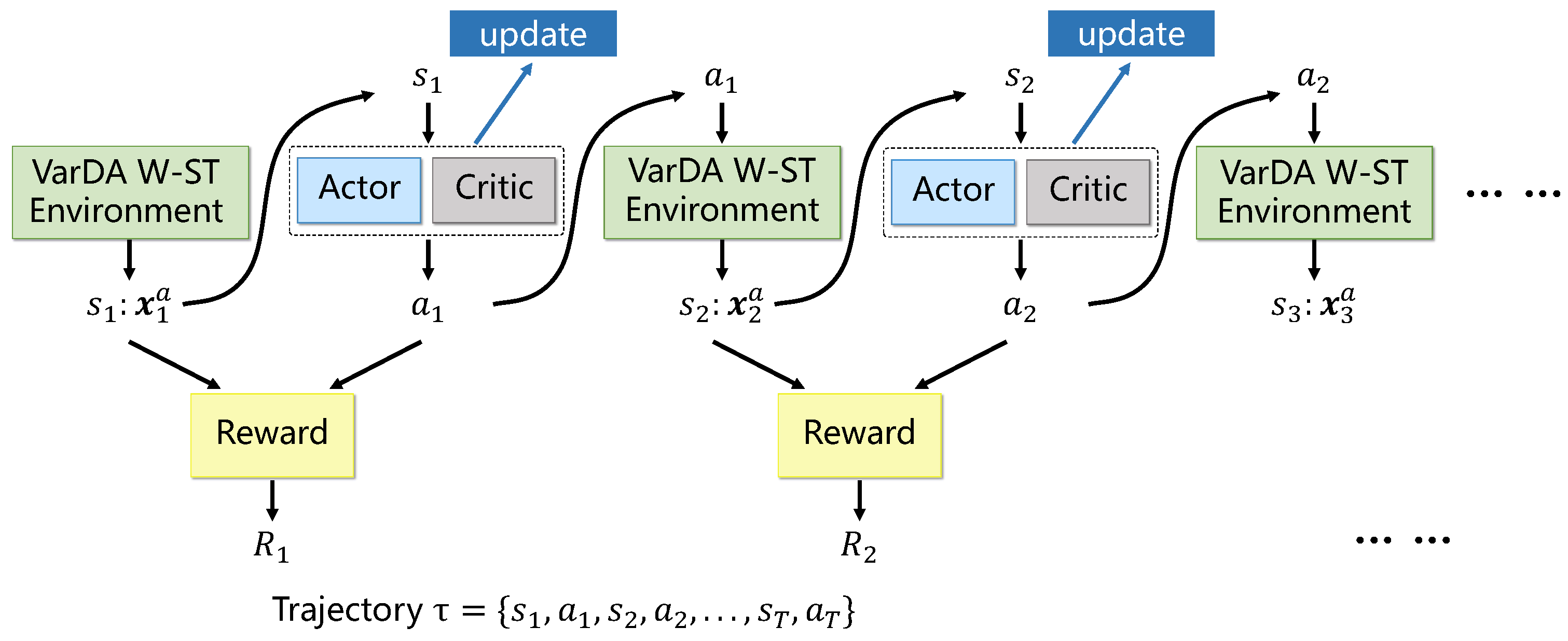
• Reward $r(s_t,a_t,s_{t+1})$ quantifies the immediate benefit of applying action $a_t$ at state $s_t$, resulting in the new state $s_{t+1}$. This study aims to learn an adaptive variance rescaling policy that improves the quality of assimilation, thereby providing initial conditions that enhance the subsequent forecast performance. Since the effectiveness of data assimilation depends on multiple factor, the detailed formulation of r is provided in subsequent content.
• Discount factor $\gamma$ is set close to 1, as our task requires long-term planning over sequential assimilation cycles.

Setting of the Reward Function: as we have mentioned previously, the purpose of the DA system is to provide the optimal initial state for numerical weather models, thereby improving the accuracy of NWP. Therefore, the indicator for measuring the optimal initial state is the value that directly describes the performance of the DA system, while the indicator for measuring the accuracy of NWP is the value that assists in describing the quality of the result of the DA system, both of which are important components of the reward function.

To evaluate the performance of the DA system, the root mean square error (RMSE) between ${\mathbf{x}}^a$ and ${\mathbf{x}}^t$ is a general evaluation metric, where ${\mathbf{x}}^t$ can be calculated by integrating the numerical model, which is considered perfect and without model errors in our task. Thus, the following function represents the first reward:

$$\begin{array}{c}\hfill r_a=RMS{E}_a=\sqrt{{\displaystyle \frac{1}{JT}}\sum _{i=0}^T\sum _{j=1}^J{\left({\mathbf{x}}_{ij}^t-{\mathbf{x}}_{ij}^a\right)}^2}\end{array}$$

(17)

where J is the number of model state variables, T is the total time of the DA system, and $x_{ij}$ represents the jth state variable in the ith timestep.

To evaluate the accuracy of the NWP forecast, the RMSE between ${\mathbf{x}}^f$ (the forecast state predicted by the numerical model) and ${\mathbf{x}}^t$ is a typical index:

$$\begin{array}{c}\hfill r_f=RMS{E}_f=\sqrt{{\displaystyle \frac{1}{JT}}\sum _{i=0}^T\sum _{j=1}^J{\left({\left({\mathbf{x}}_j^t\right)}_i-{\left({\mathbf{x}}_j^f\right)}_i\right)}^2}\end{array}$$

(18)

Overall, the reward function R is defined as follows:

$$\begin{array}{c}\hfill R=-r_a-r_f\end{array}$$

(19)

Algorithm 1 State transition process in the VarDA W-ST environment

Input: 1: Transition Model, consisting of: ${\mathbf{y}}^o$, $\mathbf{R}$, $\mathbf{H}$, $\mathcal{H}$, ${\mathbf{B}}_{\mathrm{NMC}}$ (①), number of assimilation cycles $N_{assim}$, integration timestep $dt$, number of spatial chunks $CK$, Total time T. 2: Current State $s_t$, consisting of: ${\mathbf{x}}_t^a$ based on the Lorenz-96 model. 3: Action $a_t$, representing a spatio-temporal adaptive scaling factor vector $\mathbf{W}$. Output: State transition from $s_t$ to $s_{t+1}$ via the VarDA W-ST environment. 4: for  $t=1,2,\dots ,T$  do 5:       Observe current state: $s_t\leftarrow {\mathbf{x}}_t^a$                   (Step (1)) 6:       Generate action: $a_t\leftarrow \mathbf{W}=[w_1,w_2,\dots ,w_{ck}]$                (Step (2)) 7:       Normalize NMC $\mathbf{B}$ globally: ${\mathbf{B}}_{\mathrm{norm}}\leftarrow \mathrm{normalize}\left({\mathbf{B}}_{\mathrm{NMC}}\right)$           (④) 8:       Apply chunk-wise rescaling: 9:       for $ck=1,\dots ,CK$ do 10:           ${\mathbf{B}}_{\mathbf{W}}^{\left(ck\right)}\leftarrow w_{ck}·{\mathbf{B}}_{norm}^{\left(ck\right)}$                         (Step (3), ⑤) 11:     end for (complete ${\mathbf{B}}_{\mathbf{W}}$ with all rescalings) 12:     for $i=1,2,\dots ,N_{assim}$ do 13:           Advance to the background state at time $t+1$: ${\mathbf{x}}_{t+1}^b\leftarrow \mathrm{RK}4({\mathbf{x}}_t^a,dt)$      (②) 14:           Compute the innovation at time $t+1$: ${\mathbf{d}}_{t+1}\leftarrow {\mathbf{y}}^o-\mathcal{H}\left({\mathbf{x}}_{t+1}^b\right)$       (③) 15:           Update analysis state: ${\mathbf{x}}_{t+1}^a\leftarrow {\mathbf{x}}_{t+1}^b+{\mathbf{B}}_{\mathbf{W}}{\mathbf{H}}^T{(\mathbf{H}{\mathbf{B}}_{\mathbf{W}}{\mathbf{H}}^T+\mathbf{R})}^{-1}{\mathbf{d}}_{t+1}$         (⑥) 16:           Update state: $s_{t+1}\leftarrow {\mathbf{x}}_{t+1}^a$                 (for next cycle, ⑦) 17:     end for 18: end for 19: return  $s_{t+1}$

4.3. Actor–Critic Framework and Proximal Policy Optimization (PPO) Algorithm

This study introduces a DRL algorithm based on the PPO method under the actor–critic architecture [51], aiming to learn spatio-temporal scaling strategies for the $\mathbf{B}$-matrix in a VarDA system. The VarDA system is formulated as an interactive environment, where an agent learns optimal actions (scaling strategies) through trial-and-error interactions. The actor–critic framework jointly learns a stochastic policy (actor) and a state value function (critic), thereby improving decision quality and training efficiency. Specifically, we adopt policy gradient methods to optimize the policy directly instead of indirectly deriving it from an approximated value function [52]. The objective is to maximize the expected cumulative reward by updating the policy via gradient ascent, as defined by the following expression:

$$\begin{array}{c}\hfill {\nabla }_{\theta }J\left({\pi }_{\theta }\right)=\underset{\tau \sim {\pi }_{\theta }\left(\tau \right)}{\mathbb{E}}\left[{\sum }_{t=0}^T{\nabla }_{\theta }log{\pi }_{\theta }(a_t\mid s_t)R\left(\tau \right)\right]\end{array}$$

(20)

where $\theta$ denotes the parameters of the policy network. In the customized environment VarDA W-ST, a trajectory $\tau =s_1,a_1,s_2,a_2,\dots ,s_T,a_T$ (as illustrated in Figure 2) denotes a sequence of states and actions executed by the agent under policy ${\pi }_{\theta }$. The probability of generating a trajectory under the current policy is denoted by ${\pi }_{\theta }\left(\tau \right)$, and ${\pi }_{\theta }(a_t\mid s_t)$ represents the probability of selecting action $a_t$ in state $s_t$. The cumulative reward associated with the trajectory is defined as $R\left(\tau \right)={\sum }_{t=0}^{T}r(s_t,a_t)$.

Why Choose PPO? In this study, we adopt policy gradient methods to optimize the policy directly, offering a substantial improvement in computational efficiency over traditional approaches that first approximate the value function before deriving the policy indirectly. Modern policy gradient algorithms can be broadly classified into two categories: on-policy methods, such as Advantage Actor–Critic (A2C), Trust Region Policy Optimization (TRPO), and PPO; and off-policy methods, including Deep Deterministic Policy Gradient (DDPG), Twin Delayed Deep Deterministic Policy Gradient (TD3), and Soft Actor–Critic (SAC) [53]. Off-policy methods, such as DDPG leverage an experience replay buffer to enhance sample efficiency by reusing past interactions. However, they are highly sensitive to hyperparameter tuning, such as exploration noise and the soft target update rate. Poorly tuned hyperparameters can result in unstable training dynamics and even policy collapse [52]. In contrast, PPO improves training stability through the incorporation of importance sampling and a clipping mechanism. Specifically, PPO utilizes trajectory data collected from an earlier policy to compute the probability ratio between new and old policies. By applying a clipping constraint, PPO prevents excessively large policy updates, thereby mitigating instability and enhancing robustness [54]. Additionally, PPO integrates generalized advantage estimation (GAE) and reward normalization, reducing sensitivity to hyperparameter variations and ensuring adaptability across diverse tasks [53,55,56]. Given these advantages, we adopt PPO as the policy optimization method, achieving a balance between training stability and computational efficiency while minimizing the need for extensive hyperparameter tuning and ultimately improving the reproducibility of our experiments.

4.4. Implementation Details in the DRL-AST Method

As illustrated in Figure 3, the overall architecture is composed of the following core components:

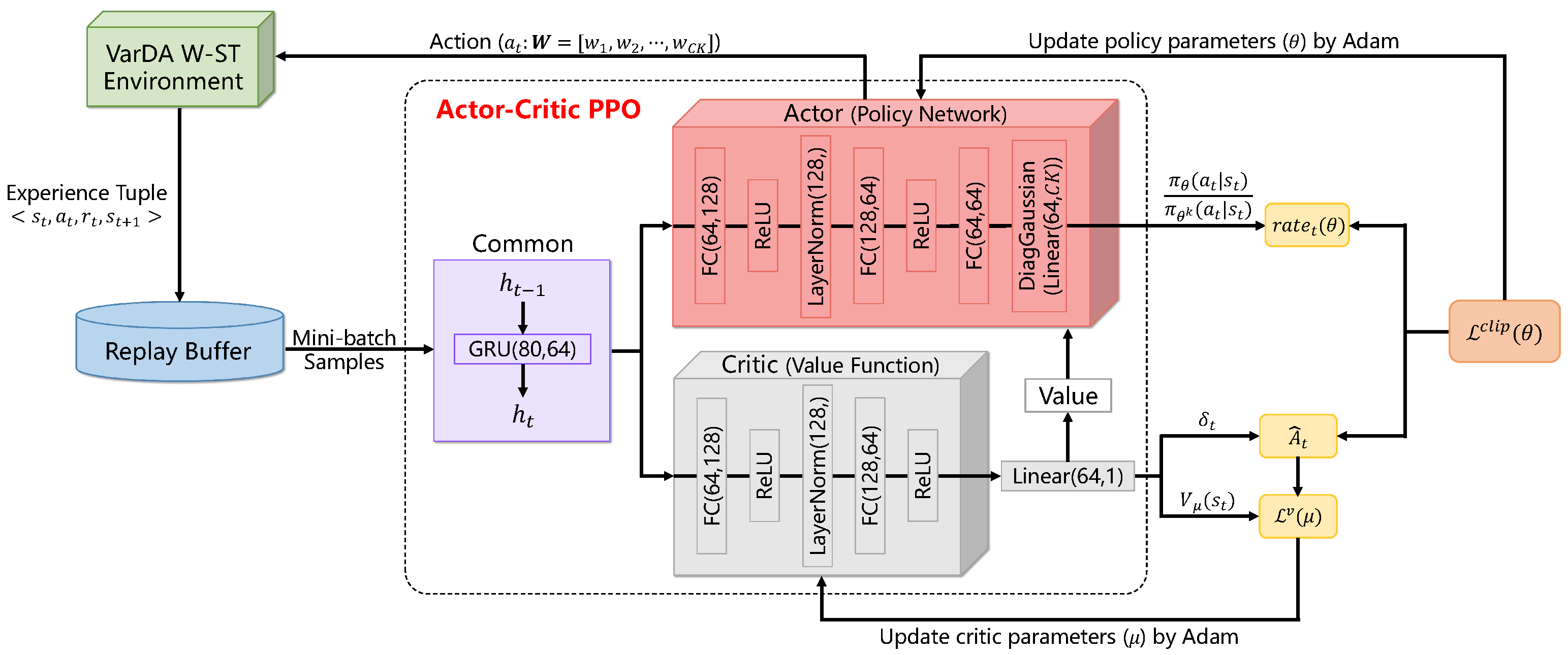
• GRU-Based Encoder (Common Module): a shared gated recurrent unit (GRU) encoder [57] is used to capture temporal dependencies in the input state sequence. At each timestep t, it updates the hidden state $h_t$ based on the previous hidden state $h_{t-1}$. The resulting representation is fed into both the actor and critic networks. This shared structure helps extract temporal features and improves training stability.
• Actor (Policy Network): the actor network receives the encoded state $h_t$ and passes it through fully connected layers with ReLU activation [58] and LayerNorm normalization [59]. The fully connected layers perform linear mappings from state features to the action space. ReLU introduces nonlinearity, and LayerNorm stabilizes training. The final layer outputs the mean and log standard deviation of a diagonal Gaussian distribution with dimension $CK$. An action $a_t=\mathbf{W}=[w_1,w_2,\dots ,w_{CK}]$ is then sampled from this distribution to produce the adaptive scaling vector.
• Critic (Value Network): the critic receives the encoded state $h_t$ and a similar architecture with the actor. It outputs a scalar value $V_{\mu }\left(s_t\right)$, representing the expected cumulative reward from state $s_t$. This value is used as a baseline to estimate the advantage ${\widehat{A}}_t$, which is essential for guiding policy improvement during training.
• Replay Buffer: following each interaction, the agent receives the next state $s_{t+1}$ and a scalar reward $r_t=R(s_t,a_t)$, which reflects the improvement in assimilation quality resulting from taking action $a_t$ in state $s_t$. The experience tuple $\langle s_t,a_t,r_t,s_{t+1}\rangle$ is temporarily stored in a replay buffer. During training, the agent samples mini-batches of these collected experiences to update the policy and value networks. This strategy improves sample efficiency and reduces the effects of temporal correlation in sequential data, thereby enhancing training stability.

The actor network is updated by maximizing a clipped surrogate objective defined by the PPO algorithm. This formulation constrains the magnitude of policy updates, ensuring training stability. The surrogate loss is given by the following:

$${\mathcal{L}}^{clip}\left(\theta \right)=\sum _{(s_t,a_t)}\min \left({\mathrm{rate}}_t\left(\theta \right)·{\widehat{A}}_t,\mathrm{clip}({\mathrm{rate}}_t\left(\theta \right),1-\zeta ,1+\zeta )·{\widehat{A}}_t\right)$$

(21)

where $rat{e}_t\left(\theta \right)={\displaystyle \frac{{\pi }_{\theta }\left(a_t\mid s_t\right)}{{\pi }_{{\theta }^k}\left(a_t\mid s_t\right)}}$ is the probability ratio between the current (${\pi }_{\theta }$) and previous (${\pi }_{{\theta }^k}$) policies for the action $a_t$ taken in state $s_t$. The advantage estimate ${\widehat{A}}_t$ quantifies how much better an action is compared to the critic’s expected return and is derived using the GAE method. The clipping function restricts policy updates to a trust region defined by $\zeta$, which is typically set to 0.2, preventing large deviations in policy updates.

The critic network, parameterized by $\mu$, is trained to minimize the discrepancy between the predicted value $V_{\mu }\left(s_t\right)$ and the target return ${\widehat{R}}_t={\widehat{A}}_t+V_{\mu }\left(s_t\right)$. The advantage is computed as a weighted sum of temporal-difference (TD) errors [51], where $\lambda$ is a decay factor controlling the bias-variance trade-off:

$${\widehat{A}}_t={\delta }_t+\left(\gamma \lambda \right){\delta }_{t+1}+{\left(\gamma \lambda \right)}^2{\delta }_{t+2}+\cdots$$

(22)

where ${\delta }_t$ denotes the TD error, which quantifies the deviation between the predicted value and the bootstrapped return from the next state.

Accordingly, the value loss is given by the following:

$${\mathcal{L}}^v\left(\mu \right)={\left(V_{\mu }\left(s_t\right)-{\widehat{R}}_t\right)}^2$$

(23)

Both the actor and critic networks are optimized using the Adam optimizer. The key hyperparameters used in DRL-AST training are summarized in

Table 2. Hyperparameters utilized in DRL-AST training.

Parameter	Value	Description
Scaling factor bounds $(l,u)$	$(1\times {10}^{-4},3.6)$	Range for the action space in DRL-AST
Learning rate	$7\times {10}^{-4}$	Adam optimizer learning rate
Batch size	128	Number of samples per training batch
PPO epochs	4	Number of PPO update steps per iteration
Total training steps	${10}^7$	Total environment steps for training
Discount factor ($\gamma$)	0.998	Future reward discount factor
GAE parameter ($\lambda$)	0.95	Smoothing factor in GAE
PPO clip parameter ($\zeta$)	0.2	Clipping threshold in PPO
Entropy coefficient	0.01	Entropy regularization for exploration
Value loss coefficient	0.5	Weight of value function loss
Max gradient norm	0.5	Gradient clipping threshold

and are empirically selected to ensure stable convergence and sample-efficient policy learning.

5. Experimental Results

5.1. Baselines

Our study aims to improve the consistency between the initial conditions and the numerical model dynamics by adaptively rescaling the static B-matrix within the VarDA framework, ultimately facilitating enhanced forecast performance without incurring additional computational costs. To achieve this, we compare our method against two representative baselines:

1.

Empirical variance rescaling by a constant factor (named CON for short): this method is the most widely used in operational VarDA systems, recognized for its high assimilation performance and straightforward implementation. Despite its lack of a rigorous theoretical foundation, extensive validation in operational environments has established it a practical and reliable benchmark.

2.

An observation-dependent spatio-temporal update vector named CUTE reported by the authors of [31] (named CUTE-ST for short): CUTE-ST has been shown to outperform traditional adaptive techniques in both theoretical and practical evaluations. By leveraging background-observation error covariance within the existing VarDA cycle, it realizes spatio-temporal adaptivity in the B-matrix without introducing additional computation, rendering it an efficient and suitable baseline for comparison.

While other advanced methods exist, they were excluded from our comparative analysis due to specific limitations. The LSTM-based approach proposed by Cheng et al. [39], although an innovative application of DL in DA as described in Section 2, is not directly applicable to the diagnosis of the B-matrix. Additionally, hybrid DA methods can enhance performance by integrating ensemble-based flow-dependent covariances with static background error covariances. However, their primary drawback is the substantial computational cost associated with a larger ensemble size. Given that our study focuses on achieving adaptive variances adjustment in the B-matrix without increasing computational burdens, these two alternative methods were not included as control baselines.

The basic setup and introduction of the two baselines are presented below.

1.

CON: this baseline meticulously selects a specified constant factor within the range of 0.05 to 3.16 through an extensive series of empirical experiments. It is imperative to underscore that in instances where the observational error attains a conspicuous magnitude indicative of its unreliability, the initial value should be set to 0. However, given that the weight is contingent upon the inverse of the variance, the utilization of 0 as the denominator is precluded. Consequently, our study employs a suitably diminutive value of 0.05. The upper limit is derived from the paradigm presented by the authors of [60], wherein the forgetting factor ($\rho$, following the original notation therein) spans the interval of 0.1 to 1, thereby resulting in a variance inflation factor ($\alpha ={\rho }^{-1/2}$) that ranges from 1 to 3.16. To balance computational cost and resolution, the incremental step size for value traversal was set to 0.05.

2.

CUTE-ST: under the assumption of perfect knowledge of the $\mathbf{R}$-matrix and $\mathcal{H}$, this baseline reutilizes observations and takes the error covariance of ${\mathbf{x}}^b$ and ${\mathbf{y}}^o$—that is, Cov(${ϵ}_{{\mathbf{x}}^b}$, ${ϵ}_{{\mathbf{y}}^o}$)—into account within the iterative process of the covariance refinement. This algorithm enhances the posterior state estimation while simultaneously improving the structure of the comprehensive $\mathbf{B}$-matrix. Although Cheng et al. [39] also introduced the PUB method, CUTE is adopted as the control experiment in this study due to its superior assimilation performance when the initial $\mathbf{B}$-matrix is arbitrarily specified under sufficient observational conditions.

5.2. Evaluation Metrics

We quantitatively assess performance based on the following metrics:

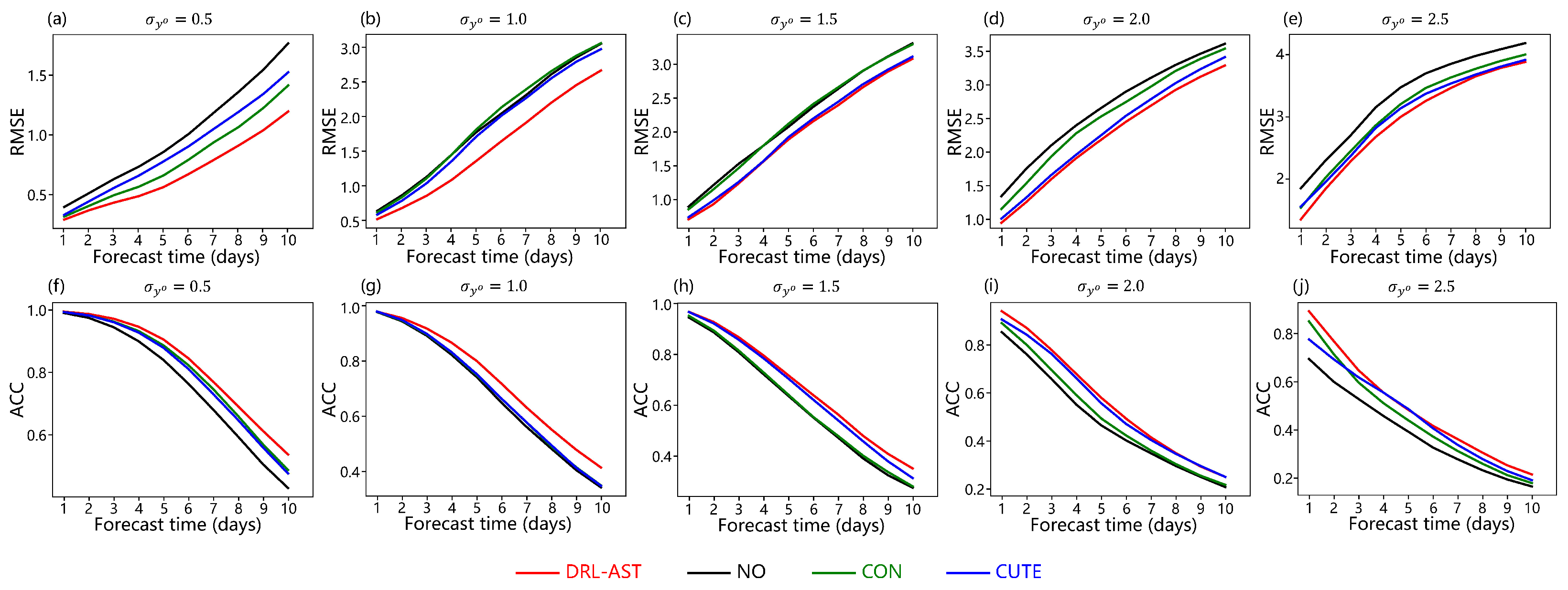
• $RMS{E}_a$: a standard metric for directly assessing the accuracy of the analysis state generated by the DA system.
• $RMS{E}_f$: continuous predictions initialized from the analysis state are performed over 72 h, 7 days, and 15 days without additional data assimilation. The resulting forecast performance is used to directly evaluate the dynamical consistency and adaptability of the initial conditions provided by the DA system.

5.3. Quantitative Results

5.3.1. Basic Settings of VarDA System

Firstly, the numerical model settings follow the protocol detailed in Section 4.1. The synthetic observations are obtained from the ‘true’ state by adding the Gaussian noise of the zero mean and covariance matrix $\mathbf{R}$, where observation errors are supposed to be spatially independent and uncorrelated—that is, the $\mathbf{R}$-matrix is proportional to an identity matrix ($\mathbf{R}={\sigma }_{y^o}^2\mathbf{I}$), where the standard deviations of observation errors ${\sigma }_{y^o}$ are set to 0.5, 1.0, 1.5, 2.0, and 2.5, respectively. The observation interval is the same as the integration time step of the model.

5.3.2. Sensitivity to Hyperparameters

We study the effect of two control parameters here: the time variation and the number of rescaling factors selected by the agent at once. Experiments were conducted on a workstation within the amd_512 queue of the ZC-M6 supercomputing system. The workstation is equipped with an NVIDIA GeForce RTX 3090 GPU (24 GB GDDR6X; NVIDIA Corp., Santa Clara, CA, USA) and an AMD EPYC 7H12 64-core processor (2.6 GHz, 512 GB RAM; Advanced Micro Devices, Inc., Santa Clara, CA, USA). The VarDA DRL-AST method was implemented using PyTorch (v1.10.0, https://pytorch.org, accessed on 30 January 2024) with Python 3.7 [61].

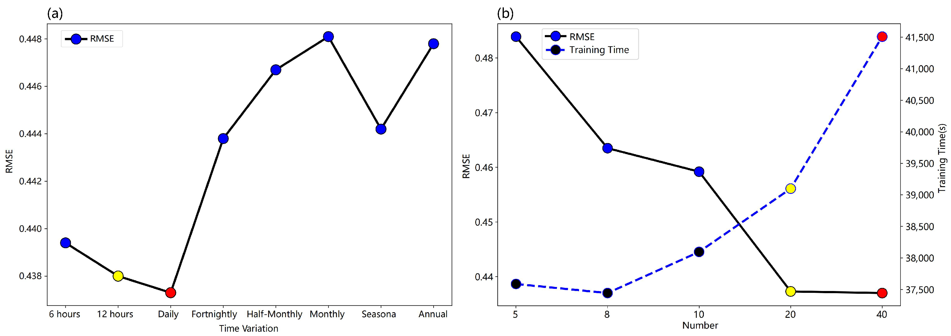
• Time variation: seven controlled experiments were conducted to compare and evaluate the effect of time variations on assimilation performance and the training cost of neural network models, including 6 h, 12 h, daily, semi-monthly, monthly, seasonal, and annual intervals. The experimental results are shown in Figure 4a, revealing that assimilation performance is optimal when the variance is rescaled daily (as indicated by the value in the solid red dot). There is no notable change in assimilation performance with higher rescaled frequency, which may be related to the inherent stability of the Lorenz-96 model itself. Thus, the daily change is deemed sufficient to reflect the flow-dependent characteristics of the model. Then, our study opts for daily variation in follow-up experiments.
• The number of rescaling factors: guided by the inherent characteristics of the Lorenz-96 model variables, where 40 variables are equidistant around the equator, we explore a concept called ‘chunking’, in which a block corresponds to a rescaling factor and adjacent variables share the same factor. Our experimentation encompasses block sizes of 5, 8, 10, 20, and 40 because there are 40 variables in our study for even distribution. Remarkably, as shown in Figure 4b, an escalation in the number of blocks positively correlates with improved assimilation performances. Nevertheless, transitioning from 20 to 40 blocks yields only marginal gains in assimilation performance, while increasing model training costs. Consequently, this study adopts a balanced approach, opting for 20 blocks ($CK=20$).

Figure 4. Experimental results of sensitivity to (a) time variation and (b) the number of rescaling factors. Solid red dots represent optimal results, and solid yellow dots represent suboptimal results.

Figure 4. Experimental results of sensitivity to (a) time variation and (b) the number of rescaling factors. Solid red dots represent optimal results, and solid yellow dots represent suboptimal results.

We take 5 times training with different random seeds, and the mean returns of the model in the training phase are shown in Figure 5. This result shows that our method can achieve stable convergence every time.

5.3.3. Performance of DA System and Model Forecasting

Four assimilation control experiments were conducted: NO without rescaling; CON with a constant rescaling factor; CUTE-ST updates the entire construction of the B-matrix at the end of each iteration; DRL-AST has spatially and temporally varying adaptive rescaling factors, as described in Section 4. To ensure the reliability of the experimental results and to eliminate random effects, each control experiment was independently repeated 50 times, with the mean value was reported as the final result, as summarized in

Table 3. Assimilation and forecast results. Values are displayed as an average of 50 experiments, where performance is expressed as ‘mean ± standard deviation’, and the improvement/reduction ratio relative to the NO method is reported as ‘mean ± standard deviation’. Bold indicates optimal results, and an underline indicates suboptimal results.

Metrics	Time	${\mathit{\sigma }}^{{\mathit{y}}^{\mathit{o}}}$	Methods
			NO	CON	CUTE-ST	DRL-AST (Ours)
RMSEa	5 years	0.5	0.36 ± 0.0006	0.27 ± 0.0011, 24.46% ± 0.33%	0.29 ± 0.0006, 18.12% ± 0.21%	0.25 ± 0.0006, 29.47% ± 0.20%
		1.0	0.53 ± 0.0017	0.51 ± 0.0018, 3.36% ± 0.37%	0.52 ± 0.0011, 2.07% ± 0.37%	0.44 ± 0.0016, 17.57% ± 0.42%
		1.5	0.75 ± 0.0057	0.74 ± 0.0049, 1.12% ± 1.04%	0.63 ± 0.0021, 15.82% ± 0.75%	0.63 ± 0.0021, 15.71% ± 0.70%
		2.0	1.17 ± 0.0188	0.97 ± 0.0062, 16.97% ± 1.33%	0.86 ± 0.0090, 26.18% ± 1.46%	0.83 ± 0.0037, 29.00% ± 1.18%
		2.5	1.80 ± 0.0252	1.20 ± 0.0078, 33.42% ± 1.06%	1.37 ± 0.0187, 23.69% ± 1.54%	1.08 ± 0.0035, 39.93% ± 0.86%
RMSEf	72 h	0.5	0.72 ± 0.20	0.67 ± 0.17, 6.61% ± 5.77%	0.68 ± 0.19, 6.40% ± 6.51%	0.58 ± 0.18, 20.10% ± 8.86%
		1.0	1.21 ± 0.30	1.19 ± 0.35, 2.18% ± 6.45%	1.11 ± 0.29, 8.00% ± 4.39%	0.94 ± 0.24, 21.80% ± 3.40%
		1.5	1.60 ± 0.45	1.54 ± 0.33, 1.74% ± 7.09%	1.33 ± 0.32, 15.71% ± 6.08%	1.32 ± 0.29, 15.62% ± 6.06%
		2.0	2.18 ± 0.61	2.03 ± 0.49, 5.89% ± 5.03%	1.74 ± 0.46, 19.84% ± 3.41%	1.74 ± 0.45, 19.55% ± 4.11%
		2.5	2.61 ± 0.57	2.26 ± 0.47, 13.07% ± 3.89%	2.32 ± 0.54, 11.29% ± 5.31%	1.96 ± 0.44, 24.62% ± 3.54%
	7 days	0.5	1.91 ± 0.43	1.76 ± 0.44, 8.20% ± 3.50%	1.87 ± 0.46, 2.62% ± 4.58%	1.56 ± 0.47, 19.06% ± 7.63%
		1.0	2.39 ± 0.43	2.46 ± 0.52, −2.42% ± 6.74%	2.34 ± 0.41, 2.02% ± 3.38%	2.07 ± 0.42, 13.99% ± 5.43%
		1.5	2.70 ± 0.47	2.72 ± 0.47, −0.66% ± 4.33%	2.51 ± 0.44, 7.02% ± 4.34%	2.52 ± 0.39, 6.08% ± 6.80%
		2.0	3.15 ± 0.56	3.03 ± 0.49, 3.27% ± 5.23%	2.84 ± 0.45, 9.38% ± 3.01%	2.83 ± 0.45, 9.53% ± 7.61%
		2.5	3.33 ± 0.41	3.29 ± 0.35, 1.04% ± 3.09%	3.05 ± 0.46, 8.78% ± 6.16%	3.02 ± 0.46, 9.65% ± 3.88%
	15 days	0.5	3.34 ± 0.34	3.29 ± 0.31, 1.57% ± 2.56%	3.31 ± 0.37, 1.01% ± 2.73%	3.06 ± 0.35, 8.51% ± 3.21%
		1.0	3.78 ± 0.31	3.76 ± 0.36, 0.52% ± 2.01%	3.63 ± 0.31, 3.88% ± 1.44%	3.52 ± 0.32, 6.98% ± 1.69%
		1.5	3.94 ± 0.35	3.89 ± 0.33, 1.05% ± 2.66%	3.74 ± 0.34, 4.87% ± 1.79%	3.79 ± 0.34, 3.59% ± 3.28%
		2.0	4.07 ± 0.31	4.05 ± 0.35, 0.47% ± 2.20%	3.97 ± 0.30, 2.33% ± 1.10%	3.97 ± 0.30, 2.39% ± 1.06%
		2.5	4.21 ± 0.30	4.20 ± 0.23, 0.23% ± 1.97%	4.08 ± 0.35, 3.24% ± 2.89%	4.02 ± 0.32, 4.54% ± 2.64%

.

Comparison of the analysis states ($RMS{E}_a$): as shown in Table 3 (specifically, rows 3 to 7), the $RMS{E}_a$ results, which reflect the assimilation performance, indicate that any method for rescaling the variances of the B-matrix or reconstructing the B-matrix positively impacts the average performance of the long-term assimilation cycle, regardless of the quality of the observations. Across all tested standard deviations of observational errors, the proposed DRL-AST method consistently achieves competitive average $RMS{E}_a$ values and relatively small standard deviations over a 5-year continuous assimilation period. However, when ${\sigma }_{y^o}=1.5$, CUTE-ST exhibited slightly better improvements than DRL-AST (as shown in Table 3, row 5; although both methods achieve an $RMS{E}_a$ value of 0.63 when rounded to two decimal places, the unrounded value for CUTE-ST is marginally smaller). This may be attributed to the fact that CUTE-ST not only iteratively updates the variances of the B-matrix but also modifies its correlation structure, resulting in an additional impact on the assimilation results. For fair comparison, the settings of CUTE-ST were strictly reproduced in this study. Nevertheless, when ${\sigma }_{y^o}=0.5,1$, and $2.5$, the improvement ratio of DRL-AST remains comparable to or slightly better than that of CUTE-ST and CON. In contrast to NO, the proposed DRL-AST method demonstrates stable assimilation performances across varying observational error levels by adaptively selecting rescaling factors through spatio-temporal optimization. Furthermore, we have included a comparison of the computational time required for the 5-year assimilation cycle under different variance adjustment methods. Specifically, when the scaling factor is 1.0, NO and CON require approximately 108 s, while the adaptive variance-adjustment methods CUTE-ST and DRL-AST achieve lower average computational times of 97 s and 89 s, respectively. To further quantify the inference efficiency, each inference step of the trained DRL-AST policy requires approximately 0.14 million floating-point operations (MFLOPs), a computational cost that is negligible relative to the processing capacity of modern GPUs (e.g., 35.58 TFLOPs for an RTX 3090), and thus unlikely to incur appreciable overhead in operational DA cycles.

Comparison of the forecast states ($RMS{E}_f$): since the core objective of DA is to generate initial states that support accurate forecasting, the analysis states produced by different variance rescaling methods are used to initialize the prediction model. Forecasts are then conducted over short-term (72 h), medium-term (7 d), and long-term (15 d) periods to directly evaluate the effectiveness of each method. Table 3 (rows 8–22) presents the forecast performance of various methods within the Lorenz-96 model framework. The proposed DRL-AST method shows potential improvements, evidenced by its effective adaptation to observations with varying standard deviations and its optimized prediction performance across different forecast timescales compared to other methods. Despite DRL-AST’s slightly lower forecasting performance than CUTE-ST in the medium and long terms when ${\sigma }_{y^o}=1.5$, its optimization level remains comparable to CUTE-ST. These results are attributed to the incorporation of the GRU module in the DRL-AST policy network, which effectively memorizes historical information by encoding the temporal evolution of the Lorenz-96 model, enabling the DRL-AST policy to make spatio-temporally informed decisions during each assimilation cycle. As a result, the analysis states generated are better aligned with the forecast model dynamics, leading to enhanced forecast accuracy across varying assimilation conditions. However, the overlapping standard deviations in Table 3 suggest that the differences in performance between methods may not be statistically significant, given the limited sample size (50 experiments) and the random nature of observational errors. This is a common challenge in Lorenz-96 experiments, where ‘mean RMSE ± standard deviation’ is a widely accepted metric for evaluating DA methods [62].

Additionally, the anomaly correlation coefficient (ACC) serves as a crucial metric for evaluating the spatial consistency between forecast states and reference datasets, such as reanalysis data, in NWP [63]. ACC provides a more insightful measure of the predictive skill of numerical models, particularly in capturing large-scale atmospheric structures. Given the essential role of ACC in long-term forecast validation, we assess the impact of different variance adjustment strategies applied to the static B-matrix in VarDA. The results show that forecast errors (RMSE) increase over time for all methods, with the NO method consistently exhibiting the highest RMSE value (Figure 6). In contrast, DRL-AST achieves the lowest RMSE value, indicating that its variance adjustment strategy results in more accurate initial conditions in the VarDA process. The ACC results further highlight differences in forecast skill deterioration. While all methods experience a decline, the NO method degrades the fastest, whereas DRL-AST maintains the highest ACC, suggesting that it better preserves the structural integrity of the initial conditions, which benefits medium-range to long-range forecasts. Overall, DRL-AST outperforms other B-matrix variance adjustment strategies (CON and CUTE-ST) across different observational error levels. By optimizing the assimilation-derived initial conditions, DRL-AST improves the quality of the initial conditions for numerical models, contributing to reduced forecast errors and improved predictive skills over extended lead times.

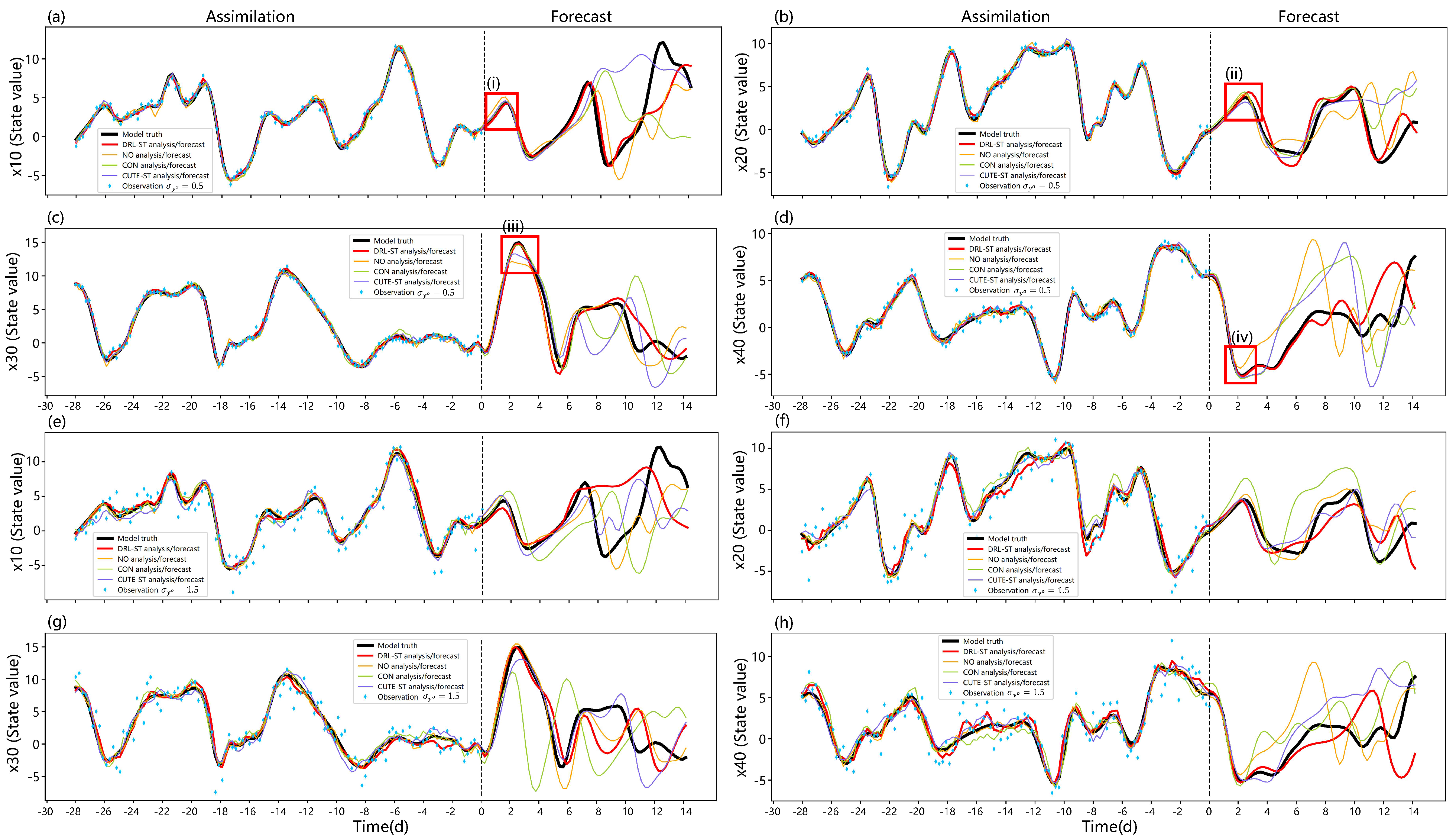
5.4. Qualitative Results

To more intuitively analyze the effect of the initial states provided by different methods on the prediction performance of the Lorenz-96 model, we refer to Figure 7. At the same starting moment when ${\sigma }_{y^o}=1.0$, different initial states are provided by applying different variance rescaling methods to the VarDA system. These initial states are then used to make predictions on eight Lyapunov time units without additional assimilation. The differences in their predictions with respect to ${\mathbf{x}}^t$ are then calculated. DRL-AST can accurately predict two Lyapunov time units (as shown in Figure 7d, highlighted in the green box), which is twice as much as the standard of the Lorenz-96 model [64]. In contrast, almost all other methods reach the error saturation point within one Lyapunov time unit. This result underscores the effectiveness of DRL-AST in extending the predictability of chaotic systems. To further improve performance in the Lorenz-96 model and extend the effective forecast lead time, two key directions can be explored. One approach comprises refining the dynamic adaptation of B, where DRL-AST currently adjusts only the variance components. Dynamically tuning length scales could further enhance forecast stability across different atmospheric motion scales [65]. In regions where the error growth is rapid, particularly those associated with high Lyapunov exponents, an adaptive scale-rescaling strategy could be introduced to refine the off-diagonal components of B, mitigating nonphysical error amplification. Another approach involves enhancing the reinforcement learning framework to optimize DRL-AST. Refining the reward function to explicitly reinforce long-term forecast objectives—such as incorporating Lyapunov time-weighted rewards—could enable the DRL agent to learn more robust assimilation policies. Additionally, employing adaptive exploration strategies, such as entropy-regularized learning, could prevent premature convergence to suboptimal solutions, thereby improving the generalization capacity of DRL-AST [66]. These potential improvements could further strengthen DRL-AST’s adaptability in chaotic systems and provide a foundation for its application in more complex atmospheric dynamic models.

The analysis of individual variables from assimilation to model prediction illustrates the degree of alignment between the analysis state obtained from assimilation as the initial state and the numerical model. Figure 8a–d depict the scenario at ${\sigma }_{y^o}=0.5$, where the performance of the VarDA system, adjusted by various variance rescaling strategies, excels due to high-quality observations. However, at the inflection points (highlighted in red boxes), the VarDA system without variance adjustment (NO) exhibits a large forecast error. This divergence is further examined in Figure 9i–iv, which provide a magnified view of forecast trajectories around these critical points. Here, DRL-AST demonstrates the best prediction performance, with state variables that perform well maintaining accurate predictions close to the true model value for nearly 10 days ($x10,x20$, and $x30$) and even the low-performing $x40$ producing valid predictions for one week. In contrast, other methods only sustain valid predictions for 6–7 days for well-performing state variables and merely 2 days for $x40$. The large standard deviation of observations in Figure 8e–h indicates substantial observation errors, which result in varying degrees of degradation in assimilation performances. However, despite these errors, the assimilation process still preserves a time evolution similar to the model truth. Adjusting the background error variances using the DRL-AST’s adaptive variance rescaling strategy as an initial state enables effective model prediction for nearly 7 days. In comparison, other strategies can barely maintain about 2 days of effective model prediction before deviating markedly from true values and being considered invalid predictions.

This result demonstrates that DRL-AST notably extends the effective forecast lead time by adaptively optimizing B. Unlike other variance rescaling methods, DRL-AST leverages a GRU module to analyze historical assimilation states, dynamically adjusting B to enhance consistency between the analysis 3D-Var and the model’s dynamical constraints. This adaptive approach helps delay error amplification, allowing the model to maintain skillful predictions for nearly 7 days. However, the inherent instability of chaotic systems, characterized by exponential error growth within the Lyapunov timescale, imposes a fundamental limit on forecast reliability. While DRL-AST refines initial conditions to enhance short-term predictability, its impact on decadal or longer-term predictions remains uncertain, as initial condition effects diminish beyond a decade, and model biases dominate [67]. Additionally, incorporating geometric attractor theory and chaos-based methodologies offers valuable perspectives for understanding DRL-AST’s role in long-term predictions. Attractors define the long-term evolution of chaotic systems in phase space, and optimizing initial conditions through DRL-AST may enable numerical models to better align with the intrinsic attractor dynamics [68], thereby improving the stability of long-term statistical predictions. Furthermore, future research could explore the application of DRL-AST in seasonal-to-decadal (1–10 years) prediction, integrating classical and quantum neural network (QNN) modeling approaches to enhance forecast stability and generalization. QNNs exhibit promise in high-dimensional climate system modeling by refining initial conditions and mitigating error growth, thereby strengthening long-term forecast reliability while facilitating effective integration with physical models [69].

6. Discussion

6.1. The Rationality of the Full Observation

This study introduces an innovative spatio-temporal variance rescaling strategy (DRL-AST) grounded in a deep reinforcement learning framework, aiming to enhance the applicability and performance of background error variances within VarDA systems. To highlight the pivotal role of background error variances in assimilation analysis, numerical experiments were conducted under idealized full observation conditions, where all variables were observed at every location and time step. In this configuration, background error variances were shown to exert a decisive influence on the quality of the analysis state while effectively mitigating the impact of inter-variable correlations on the results.

However, full observation is often impractical in real-world applications, where observational data are typically sparse and noisy. Consequently, future research should prioritize optimizing the background error covariance matrix (B-matrix) under sparse observation scenarios. This endeavor requires not only the adaptive optimization of variances but also the careful consideration of inter-variable correlations. For instance, the iterative update of correlation functions employed in the CUTE-ST method offers a promising approach for comprehensive adjustments of the B-matrix.

Achieving these optimization goals necessitates the development of more efficient algorithms and thorough validation via numerical experiments. Such advancements are essential for extending the generality and robustness of deep-reinforcement-learning-based assimilation methods, facilitating their application in operational settings.

6.2. Feasibility and Applicability of DRL-AST in High-Dimensional NWP Systems

This study demonstrated the effectiveness of the DRL-AST method in optimizing the variance component of the B-matrix within the Lorenz-96 model. While the Lorenz-96 model serves as a well-established chaotic system that is widely used for testing DA techniques, its simplified structure—lacking vertical stratification and comprehensive physical processes—limits its ability to represent the multiscale interactions present in real atmospheric systems. Therefore, to assess the operational potential of DRL-AST, it is essential to validate the method within a more complex NWP model. The Simplified Parameterizations, Primitive-Equation Dynamics (SPEEDY) model, characterized by its intermediate-scale with O(${10}^4$) variables, efficient computational performance, and simplified yet representative physical parameterization schemes (e.g., convection and radiation), serves as a practical testbed for the validation of DRL-AST under computationally tractable and dynamically richer environment conditions [70]. Further transitioning to the Weather Research and Forecasting (WRF) model, with its high-resolution simulation capability, flexible physical parameterizations, and the ability to assimilate real-world observations, provides a suitable platform for evaluating the adaptability and robustness of DRL-AST in realistic forecasting environments [71]. We provide a detailed discussion of the key considerations involved in extending DRL-AST from simplified models to more complex, high-dimensional systems below:

1.

State space expands from low to high dimensions: a key challenge in transitioning DRL-AST from the Lorenz-96 model to more complex NWP models like SPEEDY and WRF is the dramatic increase in the dimensionality of the state space. Unlike the low-dimensional structure of Lorenz-96, both the SPEEDY and WRF models simulate multivariate atmospheric states, such as temperature, wind velocity, and humidity. This substantial expansion in state dimensionality introduces computational complexity, impeding efficient RL training by exacerbating convergence difficulties, increasing computational cost, and limiting policy generalization. To mitigate these challenges, future research should explore using DL for feature extraction, enabling dimensionality reduction while retaining the key physical characteristics of the atmospheric state. Possible approaches include convolutional neural networks (CNNs) for local feature extraction, variational autoencoders (VAEs) for compact latent representations, and Transformer-based attention mechanisms to enhance long-range dependencies between atmospheric variables. These methods collectively facilitate efficient state encoding, reducing computational costs and improving the RL model’s trainability. Furthermore, to enhance training stability and computational efficiency in high-dimensional NWP models, manifold-learning-based dimensionality reduction strategies, such as principal component analysis (PCA) and locally linear embedding (LLE), may be investigated. These approaches help ensure that reduced state representations retain essential physical information while minimizing redundant computations. Additionally, incorporating multi-scale feature fusion networks could further improve DRL-AST’s adaptability to diverse dynamical regimes, ensuring robust policy generalization across varying meteorological conditions. After policy inference, an inverse mapping technique may be employed to reconstruct the full atmospheric state from the reduced feature space, allowing RL-driven optimization to be effectively applied to SPEEDY and WRF models. This approach avoids direct RL applications in high-dimensional spaces, alleviating computational bottlenecks and enhancing training stability.

2.

Selecting a collaborative data assimilation system: to validate DRL-AST beyond idealized testing, we plan to first implement it within the SPEEDY model and subsequently extend it to the WRF model. The Parallel Data Assimilation Framework (PDAF) supports 3D-Var, EnKF, and hybrid methods, and its modular design facilitates efficient coupling with SPEEDY for DA experiments [72]. The WRF Data Assimilation (WRFDA) system offers a comprehensive suite of DA techniques and is tightly integrated with WRF, supporting the assimilation of diverse real-world observations to improve initial conditions [73]. For this study, we consider 3D-Var as the baseline assimilation framework due to its computational efficiency and suitability for frequent RL-environment interactions. Unlike four-dimensional variational assimilation (4D-Var) and EnKF, which involve high computational costs, 3D-Var employs a static B, allowing for rapid gradient-based optimization. However, static B cannot dynamically adapt to evolving weather regimes, potentially resulting in assimilation errors, particularly in rapidly changing systems such as deep convection and tropical cyclones. By leveraging DRL-AST to adaptively optimize the variance component of B, we anticipate improving 3D-Var’s performance across different meteorological conditions.

3.

Design and optimization of the action space: the DRL-AST action space must align with the formulation of B in the intermediate-to-complex DA system, such as those employed for SPEEDY and WRF models. Instead of storing B explicitly as a full-rank matrix, DA frameworks like PDAF and WRFDA utilize a control variable transform (CVT) approach to model B [18]. This approach decomposes B into key statistical components, including variances (${\sigma }^2$), eigenvectors, eigenvalues, and horizontal/vertical length scales. These elements provide a compact yet accurate approximation of B, preserving its essential statistical characteristics while substantially reducing storage demands and computational costs. Therefore, in experiments involving these DA systems, the action space of DRL-AST is formulated as a vector comprising spatially adaptive variance scaling factors at time step $t-1$. These factors govern the variance of different control variables across distinct regions and are dynamically adjusted by the RL agent to optimize assimilation performance. At each subsequent time step, this vector evolves, enabling a temporally adaptive adjustment mechanism. The spatial distribution of variance in B is influenced by multiple factors, including topography, large-scale circulation patterns, observational network density, and model errors. For instance, complex terrain (e.g., mountainous regions) often amplifies local dynamical processes, resulting in increased variance estimates, while observation-sparse regions such as oceans may suffer from underestimated or overestimated background errors. To identify an appropriate spatial partitioning scheme—whether based on latitude, topography, or meteorological considerations—we will draw upon literature reviews, sensitivity experiments, and data-driven statistical analyses. Furthermore, since these DA systems represent B through CVT, future extensions could refine horizontal and vertical length scales and other key components by expanding the action space. This would enable the more precise spatio-temporal tuning of B, improving variational assimilation accuracy.

4.

Bridging idealized and operational reward functions: a key challenge in extending DRL-AST from idealized environments to intermediate-to-complex NWP systems lies in constructing reward functions that remain valid when the true state of the atmosphere is not observable, as is typical in operational settings. A widely adopted solution in AI for Earth system science is to use reanalysis datasets, such as the fifth-generation ECMWF reanalysis dataset (ERA5), as proxies for the true state during training and evaluation [37]. Although ERA5 has limitations—including coarse spatial resolution and assimilation-induced biases—it provides a physically consistent and globally accessible benchmark. For high-resolution applications, such as extreme precipitation nowcasting, more localized observational datasets, including in-situ station data, radar reflectivity, and radar-derived precipitation estimates, are commonly used to approximate the true state at fine spatial and temporal scales [74,75]. These data sources serve as high-quality reference signals for constructing reward functions in DRL settings, enabling training under realistic observability constraints. By leveraging such datasets, DRL-AST can be trained in a way that respects the observational constraints of real-world NWP systems while maintaining physical realism, thereby improving its transferability from idealized testbeds (e.g., Lorenz-96) to more complex models such as SPEEDY and WRFDA.

5.

Scalability of DRL-AST in the 4D-Var framework: following the validation of DRL-AST within the WRF model, its scalability to the 4D-Var framework warrants further investigation. In 4D-Var, while B is implicitly adjusted through the assimilation window, B remains static at the initial time of each assimilation window. Thus, the adaptive variance scaling strategy learned in 3D-Var could be applied to optimize the specification of B at the beginning of each assimilation window in 4D-Var. Moreover, future studies may involve fine-tuning the RL policy within the 4D-Var context, leveraging the properties of error propagation to achieve optimal assimilation performance across extended assimilation windows. However, to fully adapt to the unique characteristics of 4D-Var, the further fine-tuning of the RL policy may be required to enhance assimilation performance.

In summary, extending DRL-AST from low-dimensional systems to high-dimensional NWP models is feasible, yet this necessitates targeted adaptations. Overcoming these challenges will pave the way for DRL-AST to enhance intelligent DA techniques, expand its operational applicability, and ultimately improve the accuracy and reliability of numerical weather predictions.

7. Conclusions

This study proposes a deep reinforcement learning-based strategy, DRL-AST, leveraging a GRU-enhanced actor–critic framework for spatio-temporally adaptive variances rescaling in the VarDA system. The method formalizes the variance adjustment of the B-matrix—estimated via the NMC method—as an MDP, in which the analysis state ${\mathbf{x}}_t^a$ serves as the environment state. A policy network is trained using the PPO algorithm to generate a chunk-wise rescaling vector $\mathbf{W}=[w_1,\dots ,w_{ck}]$ to produce an adaptively rescaled matrix ${\mathbf{B}}_{\mathbf{W}}$. This rescaled matrix is then used in the VarDA system to compute the updated analysis state. The resulting ${\mathbf{x}}_t^a$ serves as the initial condition for the next forecast cycle, thereby completing the sequential forecast–assimilation cycle. This framework enables dynamic, cycle-wise variance rescaling driven by the evolving forecast state, thereby enhancing the integration of observations and contributing to improved forecast accuracy across assimilation cycles.

Compared to the constant rescaling factor in the CON method and the semi-adaptive strategy of CUTE-ST, which requires the manual tuning of the parameter $\alpha$ within the range of 0 to 1, DRL-AST achieves a fully adaptive spatio-temporal variance rescaling. Numerical experiments demonstrate that DRL-AST provides competitive forecast skill across different observational error levels by generating initial conditions that are more dynamically consistent.

After training, DRL-AST can be seamlessly integrated into the assimilation system as a forward computation step without incurring additional computational costs. This feature allows DRL-AST to maintain computational efficiency while enhancing forecast performance, making it well suited for long-term numerical forecasting tasks. Further analyses reveal that the GRU module in the DRL-AST policy network effectively captures the historical evolution of assimilation states, thereby implicitly learning the dynamical structure of the forecast model. The experimental results indicate that the initial state optimized by DRL-AST extends the effective prediction skill of the forecast model to approximately two Lyapunov times, whereas other methods typically exhibit rapid error growth and saturation after a single Lyapunov time. This advantage is particularly evident in predictions following univariate assimilation analysis. Overall, the DRL-AST-enhanced VarDA system provides initial conditions that better align with the dynamical constraints of numerical models, ensuring improved stability and accuracy in long-term forecasts.

Future research will focus on extending DRL-AST to high-dimensional NWP models, particularly within complex frameworks such as WRF. To enhance operational feasibility, DL-based dimensionality reduction techniques will be explored to mitigate computational costs. Additionally, DRL-AST’s policy network can be transferred to 4D-Var to broaden its applicability. However, given the high computational cost of 4D-Var, ensuring efficient RL training remains a critical challenge.

In summary, DRL-AST is an efficient and scalable spatio-temporally adaptive data assimilation strategy that not only demonstrates competitive performance in the Lorenz-96 model but also holds great potential for extension to high-dimensional numerical weather prediction systems. Future research will further optimize its computational efficiency, enhance its adaptability to complex atmospheric systems, and explore its applicability across various DA systems.

References

- Bauer, P.; Thorpe, A.; Brunet, G. The quiet revolution of numerical weather prediction. Nature 2015, 525, 47–55. [Google Scholar] [CrossRef] [PubMed]
- Abbe, C. The physical basis of long-range weather forecasts. Mon. Weather Rev. 1901, 29, 551–561. [Google Scholar] [CrossRef]
- Verhulst, F. Nonlinear Differential Equations and Dynamical Systems; Springer Science & Business Media: Berlin/Heidelberg, Germany, 2012. [Google Scholar]
- Richardson, L.F. Weather Prediction by Numerical Process; Cambridge University Press: Cambridge, UK, 1922. [Google Scholar]
- Wolf, A.; Swift, J.B.; Swinney, H.L.; Vastano, J.A. Determining Lyapunov exponents from a time series. Phys. D Nonlinear Phenom. 1985, 16, 285–317. [Google Scholar] [CrossRef]
- Arnol’d, V.I. Small denominators and problems of stability of motion in classical and celestial mechanics. Russ. Math. Surv. 1963, 18, 85. [Google Scholar] [CrossRef]
- Arnold, V.I. Geometrical Methods in the Theory of Ordinary Differential Equations; Springer Science & Business Media: Berlin/Heidelberg, Germany, 2012. [Google Scholar]
- Pecora, L.M.; Carroll, T.L. Synchronization in chaotic systems. Phys. Rev. Lett. 1990, 64, 821. [Google Scholar] [CrossRef]
- Wang, B.; Zou, X.; Zhu, J. Data assimilation and its applications. Proc. Natl. Acad. Sci. USA 2000, 97, 11143–11144. [Google Scholar] [CrossRef]
- Talagrand, O. Assimilation of observations, an introduction. J. Meteorol. Soc. Jpn. Ser. 1997, 75, 191–209. [Google Scholar] [CrossRef]
- Daley, R. Atmospheric Data Analysis; Cambridge University Press: Cambridge, UK, 1993. [Google Scholar]
- Asch, M.; Bocquet, M.; Nodet, M. Data Assimilation: Methods, Algorithms, and Applications; SIAM: Philadelphia, PA, USA, 2016. [Google Scholar]
- Gettelman, A.; Geer, A.J.; Forbes, R.M.; Carmichael, G.R.; Feingold, G.; Posselt, D.J.; Stephens, G.L.; Van den Heever, S.C.; Varble, A.C.; Zuidema, P. The future of Earth system prediction: Advances in model-data fusion. Sci. Adv. 2022, 8, eabn3488. [Google Scholar] [CrossRef]
- Carrassi, A.; Bocquet, M.; Bertino, L.; Evensen, G. Data assimilation in the geosciences: An overview of methods, issues, and perspectives. Wiley Interdiscip. Rev. Clim. Change 2018, 9, e535. [Google Scholar] [CrossRef]
- Benjamin, S.G.; Weygandt, S.S.; Brown, J.M.; Hu, M.; Alexander, C.R.; Smirnova, T.G.; Olson, J.B.; James, E.P.; Dowell, D.C.; Grell, G.A.; et al. A North American hourly assimilation and model forecast cycle: The Rapid Refresh. Mon. Weather Rev. 2016, 144, 1669–1694. [Google Scholar] [CrossRef]
- Dowell, D.C.; Alexander, C.R.; James, E.P.; Weygandt, S.S.; Benjamin, S.G.; Manikin, G.S.; Blake, B.T.; Brown, J.M.; Olson, J.B.; Hu, M.; et al. The High-Resolution Rapid Refresh (HRRR): An hourly updating convection-allowing forecast model. Part I: Motivation and system description. Weather Forecast. 2022, 37, 1371–1395. [Google Scholar] [CrossRef]
- Bannister, R.N. A review of operational methods of variational and ensemble-variational data assimilation. Q. J. R. Meteorol. Soc. 2017, 143, 607–633. [Google Scholar] [CrossRef]
- Bannister, R.N. A review of forecast error covariance statistics in atmospheric variational data assimilation. II: Modelling the forecast error covariance statistics. Q. J. R. Meteorol. Soc. A J. Atmos. Sci. Appl. Meteorol. Phys. Oceanogr. 2008, 134, 1971–1996. [Google Scholar] [CrossRef]
- Bannister, R.N. A review of forecast error covariance statistics in atmospheric variational data assimilation. I: Characteristics and measurements of forecast error covariances. Q. J. R. Meteorol. Soc. A J. Atmos. Sci. Appl. Meteorol. Phys. Oceanogr. 2008, 134, 1951–1970. [Google Scholar] [CrossRef]
- Gustafsson, N.; Bojarova, J.; Vignes, O. A hybrid variational ensemble data assimilation for the HIgh Resolution Limited Area Model (HIRLAM). Nonlinear Process. Geophys. 2014, 21, 303–323. [Google Scholar] [CrossRef]
- Tandeo, P.; Ailliot, P.; Bocquet, M.; Carrassi, A.; Miyoshi, T.; Pulido, M.; Zhen, Y. A review of innovation-based methods to jointly estimate model and observation error covariance matrices in ensemble data assimilation. Mon. Weather Rev. 2020, 148, 3973–3994. [Google Scholar] [CrossRef]
- Parrish, D.F.; Derber, J.C. The National Meteorological Center’s spectral statistical-interpolation analysis system. J. Abbr. 1992, 120, 1747–1763. [Google Scholar] [CrossRef]
- Bonavita, M.; Isaksen, L.; Hólm, E. On the use of EDA background error variances in the ECMWF 4D-Var. Q. J. R. Meteorol. Soc. 2012, 138, 1540–1559. [Google Scholar] [CrossRef]
- Bormann, N.; Bonavita, M.; Dragani, R.; Eresmaa, R.; Matricardi, M.; McNally, A. Enhancing the impact of IASI observations through an updated observation-error covariance matrix. Q. J. R. Meteorol. Soc. 2016, 142, 1767–1780. [Google Scholar] [CrossRef]
- Jung, B.-J.; Ménétrier, B.; Snyder, C.; Liu, Z.; Guerrette, J.J.; Ban, J.; Baños, I.H.; Yu, Y.G.; Skamarock, W.C. Three-dimensional variational assimilation with a multivariate background error covariance for the Model for Prediction Across Scales—Atmosphere with the Joint Effort for Data assimilation Integration (JEDI-MPAS 2.0. 0-beta). Geosci. Model Dev. 2024, 17, 3879–3895. [Google Scholar] [CrossRef]
- Wiering, M.A.; Van Otterlo, M. Reinforcement learning. Adapt. Learn. Optim. 2012, 12, 729. [Google Scholar]
- Arulkumaran, K.; Deisenroth, M.P.; Brundage, M.; Bharath, A.A. Deep reinforcement learning: A brief survey. IEEE Signal Process. Mag. 2017, 34, 26–38. [Google Scholar] [CrossRef]
- Bellman, R. A Markovian decision process. Indiana Univ. Math. J. 1957, 6, 679–684. [Google Scholar] [CrossRef]
- Derber, J.; Bouttier, F. A reformulation of the background error covariance in the ECMWF global data assimilation system. Tellus A Dyn. Meteorol. Oceanogr. 1999, 51, 195–221. [Google Scholar] [CrossRef]
- Desroziers, G.; Berre, L.; Chapnik, B.; Poli, P. Diagnosis of observation, background and analysis-error statistics in observation space. Q. J. R. Meteorol. Soc. A J. Atmos. Sci. Appl. Meteorol. Phys. Oceanogr. 2005, 131, 3385–3396. [Google Scholar] [CrossRef]
- Cheng, S.; Argaud, J.-P.; Iooss, B.; Lucor, D.; Ponçot, A. Background error covariance iterative updating with invariant observation measures for data assimilation. Stoch. Environ. Res. Risk Assess. 2019, 33, 2033–2051. [Google Scholar] [CrossRef]
- Berre, L.; Arbogast, E. Formulation and use of 3D-hybrid and 4D-hybrid ensemble covariances in the Météo-France global data assimilation system. Q. J. R. Meteorol. Soc. 2024, 150, 416–435. [Google Scholar] [CrossRef]
- Reichstein, M.; Camps-Valls, G.; Stevens, B.; Jung, M.; Denzler, J.; Carvalhais, N.; Prabhat, F. Deep learning and process understanding for data-driven Earth system science. Nature 2019, 566, 195–204. [Google Scholar] [CrossRef]
- Karniadakis, G.E.; Kevrekidis, I.G.; Lu, L.; Perdikaris, P.; Wang, S.; Yang, L. Physics-informed machine learning. Nat. Rev. Phys. 2021, 3, 422–440. [Google Scholar] [CrossRef]
- Lam, R.; Sanchez-Gonzalez, A.; Willson, M.; Wirnsberger, P.; Fortunato, M.; Alet, F.; Ravuri, S.; Ewalds, T.; Eaton-Rosen, Z.; Hu, W.; et al. Learning skillful medium-range global weather forecasting. Science 2023, 382, 1416–1421. [Google Scholar] [CrossRef]
- Zhang, Y.; Long, M.; Chen, K.; Xing, L.; Jin, R.; Jordan, M.I.; Wang, J. Skilful nowcasting of extreme precipitation with NowcastNet. Nature 2023, 619, 526–532. [Google Scholar] [CrossRef] [PubMed]
- Bi, K.; Xie, L.; Zhang, H.; Chen, X.; Gu, X.; Tian, Q. Accurate medium-range global weather forecasting with 3D neural networks. Nature 2023, 619, 533–538. [Google Scholar] [CrossRef] [PubMed]
- Cheng, S.; Quilodrán-Casas, C.; Ouala, S.; Farchi, A.; Liu, C.; Tandeo, P.; Fablet, R.; Lucor, D.; Iooss, B.; Brajard, J.; et al. Machine learning with data assimilation and uncertainty quantification for dynamical systems: A review. IEEE/CAA J. Autom. Sin. 2023, 10, 1361–1387. [Google Scholar] [CrossRef]
- Cheng, S.; Qiu, M. Observation error covariance specification in dynamical systems for data assimilation using recurrent neural networks. Neural Comput. Appl. 2022, 34, 13149–13167. [Google Scholar] [CrossRef]
- Hammoud, M.A.E.R.; Raboudi, N.; Titi, E.S.; Knio, O.; Hoteit, I. Data assimilation in chaotic systems using deep reinforcement learning. J. Adv. Model. Earth Syst. 2024, 16, e2023MS004178. [Google Scholar] [CrossRef]
- Houtekamer, P.L.; Zhang, F. Review of the ensemble Kalman filter for atmospheric data assimilation. J. Abbr. 2016, 144, 4489–4532. [Google Scholar] [CrossRef]
- Jeung, M.; Jang, J.; Yoon, K.; Baek, S.-S. Data assimilation for urban stormwater and water quality simulations using deep reinforcement learning. J. Hydrol. 2023, 624, 129973. [Google Scholar] [CrossRef]
- Zhao, J.; Guo, Y.; Lin, Y.; Zhao, Z.; Guo, Z. A novel dynamic ensemble of numerical weather prediction for multi-step wind speed forecasting with deep reinforcement learning and error sequence modeling. Energy 2024, 302, 131787. [Google Scholar] [CrossRef]
- Wu, Z.; Fang, G.; Ye, J.; Zhu, D.Z.; Huang, X. A Reinforcement Learning-Based Ensemble Forecasting Framework for Renewable Energy Forecasting. Renew. Energy 2025, 244, 122692. [Google Scholar] [CrossRef]
- Saxena, D.M.; Bae, S.; Nakhaei, A.; Fujimura, K.; Likhachev, M. Driving in dense traffic with model-free reinforcement learning. In Proceedings of the 2020 IEEE International Conference on Robotics and Automation (ICRA), Paris, France, 31 May–31 August 2020; pp. 5385–5392. [Google Scholar]
- Silver, D.; Huang, A.; Maddison, C.J.; Guez, A.; Sifre, L.; Van Den Driessche, G.; Schrittwieser, J.; Antonoglou, I.; Panneershelvam, V.; Lanctot, M.; et al. Mastering the game of Go with deep neural networks and tree search. Nature 2016, 529, 484–489. [Google Scholar] [CrossRef]
- Deng, Y.; Bao, F.; Kong, Y.; Ren, Z.; Dai, Q. Deep direct reinforcement learning for financial signal representation and trading. IEEE Trans. Neural Netw. Learn. Syst. 2016, 28, 653–664. [Google Scholar] [CrossRef] [PubMed]
- Lorenz, E.N.; Emanuel, K.A. Optimal sites for supplementary weather observations: Simulation with a small model. J. Atmos. Sci. 1998, 55, 399–414. [Google Scholar] [CrossRef]
- Kurosawa, K.; Poterjoy, J. A statistical hypothesis testing strategy for adaptively blending particle filters and ensemble Kalman filters for data assimilation. Mon. Weather Rev. 2023, 151, 105–125. [Google Scholar] [CrossRef]
- Miyoshi, T. The Gaussian approach to adaptive covariance inflation and its implementation with the local ensemble transform Kalman filter. Mon. Weather Rev. 2011, 139, 1519–1535. [Google Scholar] [CrossRef]
- Sutton, R.S.; Barto, A.G. Reinforcement Learning: An Introduction; MIT Press: Cambridge, MA, USA, 1998. [Google Scholar]
- Lillicrap, T.P.; Hunt, J.J.; Pritzel, A.; Heess, N.; Erez, T.; Tassa, Y.; Silver, D.; Wierstra, D. Continuous control with deep reinforcement learning. arXiv 2015, arXiv:1509.02971. [Google Scholar]
- Duan, Y.; Chen, X.; Houthooft, R.; Schulman, J.; Abbeel, P. Benchmarking deep reinforcement learning for continuous control. In Proceedings of the ICML’16: Proceedings of the 33rd International Conference on International Conference on Machine Learning, New York, NY, USA, 19–24 June 2016; pp. 1329–1338. [Google Scholar]
- Schulman, J.; Wolski, F.; Dhariwal, P.; Radford, A.; Klimov, O. Proximal policy optimization algorithms. arXiv 2017, arXiv:1707.06347. [Google Scholar]
- Schulman, J.; Moritz, P.; Levine, S.; Jordan, M.; Abbeel, P. High-dimensional continuous control using generalized advantage estimation. arXiv 2015, arXiv:1506.02438. [Google Scholar]
- Henderson, P.; Islam, R.; Bachman, P.; Pineau, J.; Precup, D.; Meger, D. Deep reinforcement learning that matters. In Proceedings of the AAAI Conference on Artificial Intelligence, New Orleans, LA, USA, 2–7 February 2018; pp. 3207–3214. [Google Scholar]
- Cho, K.; Van Merriënboer, B.; Gulcehre, C.; Bahdanau, D.; Bougares, F.; Schwenk, H.; Bengio, Y. Learning phrase representations using RNN encoder-decoder for statistical machine translation. In Proceedings of the 2014 Conference on Empirical Methods in Natural Language Processing (EMNLP), Doha, Qatar, 25–29 October 2014; pp. 1724–1734. [Google Scholar]
- Nair, V.; Hinton, G.E. Rectified linear units improve restricted boltzmann machines. In Proceedings of the 27th International Conference on Machine Learning (ICML-10), Haifa, Israel, 21–24 June 2010; pp. 807–814. [Google Scholar]
- Ba, J.L.; Kiros, J.R.; Hinton, G.E. Layer normalization. arXiv 2016, arXiv:1607.06450. [Google Scholar]
- Nerger, L. On serial observation processing in localized ensemble Kalman filters. Mon. Weather Rev. 2015, 143, 1554–1567. [Google Scholar] [CrossRef]
- Paszke, A.; Gross, S.; Massa, F.; Lerer, A.; Bradbury, J.; Chanan, G.; Killeen, T.; Lin, Z.; Gimelshein, N.; Antiga, L.; et al. PyTorch: An Imperative Style, High-Performance Deep Learning Library. In Proceedings of the Advances in Neural Information Processing Systems, Vancouver, BC, Canada, 8–14 December 2019. [Google Scholar]
- Wang, W.; Ren, K.; Duan, B.; Zhu, J.; Li, X.; Ni, W.; Lu, J.; Yuan, T. A four-dimensional variational constrained neural network-based data assimilation method. J. Adv. Model. Earth Syst. 2024, 16, e2023MS003687. [Google Scholar] [CrossRef]
- Pegion, K.; DelSole, T.; Becker, E.; Cicerone, T. Assessing the fidelity of predictability estimates. Clim. Dyn. 2019, 53, 7251–7265. [Google Scholar] [CrossRef]
- Brajard, J.; Carrassi, A.; Bocquet, M.; Bertino, L. Combining data assimilation and machine learning to infer unresolved scale parametrization. Philos. Trans. R. Soc. A 2021, 379, 20200086. [Google Scholar] [CrossRef] [PubMed]
- Lange, H.; Craig, G.C. The impact of data assimilation length scales on analysis and prediction of convective storms. Mon. Weather Rev. 2014, 142, 3781–3808. [Google Scholar] [CrossRef]
- Haarnoja, T.; Zhou, A.; Abbeel, P.; Levine, S. Soft actor-critic: Off-policy maximum entropy deep reinforcement learning with a stochastic actor. In Proceedings of the International Conference on Machine Learning, Vancouver, BC, Canada, 10–15 July 2018; pp. 1861–1870. [Google Scholar]
- Zhou, W.; Li, J.; Yan, Z.; Shen, Z.; Wu, B.; Wang, B.; Zhang, R.; Li, Z. Progress and future prospects of decadal prediction and data assimilation: A review. Atmos. Ocean. Sci. Lett. 2024, 17, 100441. [Google Scholar] [CrossRef]
- Dutta, A.; Harshith, J.; Ramamoorthy, A.; Lakshmanan, K. Attractor inspired deep learning for modelling chaotic systems. Hum.-Centric Intell. Syst. 2023, 3, 461–472. [Google Scholar] [CrossRef]
- Jeswal, S.K.; Chakraverty, S. Recent developments and applications in quantum neural network: A review. Arch. Comput. Methods Eng. 2019, 26, 793–807. [Google Scholar] [CrossRef]
- Molteni, F. Atmospheric simulations using a GCM with simplified physical parametrizations. I: Model climatology and variability in multi-decadal experiments. Clim. Dyn. 2003, 20, 175–191. [Google Scholar] [CrossRef]
- Skamarock, W.C.; Klemp, J.B.; Dudhia, J.; Gill, D.O.; Liu, Z.; Berner, J.; Wang, W.; Powers, J.G.; Duda, M.G.; Barker, D.M.; et al. A description of the advanced research WRF model version 4. Natl. Cent. Atmos. Res. 2019, 145, 550. [Google Scholar]
- Nerger, L.; Hiller, W. Software for ensemble-based data assimilation systems—Implementation strategies and scalability. Comput. Geosci. 2013, 55, 110–118. [Google Scholar] [CrossRef]
- Barker, D.; Huang, X.-Y.; Liu, Z.; Auligné, T.; Zhang, X.; Rugg, S.; Ajjaji, R.; Bourgeois, A.; Bray, J.; Chen, Y.; et al. The weather research and forecasting model’s community variational/ensemble data assimilation system: WRFDA. Bull. Am. Meteorol. Soc. 2012, 93, 831–843. [Google Scholar] [CrossRef]
- Li, D.; Deng, K.; Zhang, D.; Liu, Y.; Leng, H.; Yin, F.; Ren, K.; Song, J. LPT-QPN: A lightweight physics-informed transformer for quantitative precipitation nowcasting. IEEE Trans. Geosci. Remote Sens. 2023, 61, 1–19. [Google Scholar] [CrossRef]
- Liu, Q.; Xiao, Y.; Gui, Y.; Dai, G.; Li, H.; Zhou, X.; Ren, A.; Zhou, G.; Shen, J. MMF-RNN: A Multimodal Fusion Model for Precipitation Nowcasting Using Radar and Ground Station Data. IEEE Trans. Geosci. Remote Sens. 2025, 63, 4101416. [Google Scholar] [CrossRef]