High-Resolution Mapping of Subsurface Sedimentary Facies and Reservoirs Using Seismic Sedimentology

Abstract

This investigation presents the current status of seismic sedimentology, along with seismic geomorphology, as applied to the high-resolution (<5 m) mapping of sedimentary facies and hydrocarbon reservoirs in the subsurface. Seismic sedimentology involves the joint investigation of seismic lithology and seismic geomorphology. The high-resolution (as thin as one meter) interpretation of depositional units on lithofacies and paleo-landforms can be achieved by following a comprehensive workflow focusing on three mandatory steps (evaluating and improving data quality; selecting right attributes, preferably 90° seismic trace with frequency fusion; and making use of horizontal resolution on stratal slices) and two optional steps (guiding interpretation with seismic models and applying machine learning techniques). Seismic sedimentology is set to improve through enhanced calibration using well and outcrop data, along with regional and local geological models. Furthermore, there will be a deeper integration between geological and geophysical disciplines, as well as advancements in high-resolution geophysical acquisition and processing techniques.

1. Introduction

In the early days of subsurface seismic technology in 1977, Vail et al. introduced seismic stratigraphy [1]. It was developed for the low-resolution (50–500 m thick) analysis of basin-scale depositional systems. So-called “seismic facies” are analyzed as a group of seismic events. Because most hydrocarbon reservoirs of sedimentary origin are typically at the seismic resolvable limit or even thinner (a couple of meters to low tens of meters, often within the width of a single seismic event), seismic facies defined by multiple seismic events are unable to describe seismically thin beds. The popular RMS amplitude attribute [2] cannot catch thickness information beyond the dominant frequency, frequently misleading interpreters in a horizontal map view. Consequently, seismic stratigraphy cannot satisfy the increasing demand for high-resolution reservoir prediction for hydrocarbon exploration and development.

After decades of extensive exploration and development, most of the more accessible hydrocarbon plays in thick reservoir sequences have been discovered. The remaining hydrocarbon potential primarily lies in thin beds, such as those less than 5 m thick, particularly in non-marine basins in China and elsewhere [3]. In response to the growing need for high-resolution thin-bed mapping in sedimentary basins, seismic sedimentology emerged in the 1990s. Posamentier [4,5,6] pioneered seismic geomorphology in the early 2000s. It aimed to interpret paleo-landforms of depositional systems using horizontal and 3D seismic displays, with a high clarity and resolution unthinkable with seismic stratigraphy. This technology is popular in the industry and has enormous potential for reducing cycle time. However, it still has room for improvement. Without emphasizing the alignment of lithology logs (e.g., gamma ray) to seismic traces, predicting lithology (e.g., sandstone, shale, and carbonates) directly from data beyond geologic models has limited utility. Also, seismic resolution is less optimal in a typical zero-phase seismic data set (an industry standard), hindering the interpretation of very thin reservoirs.

Seismic sedimentology could stretch our thin-bed mapping capability further. What is seismic sedimentology? Since Zeng et al. [7] used the word for the first time, consensus has evolved. In reservoir geophysics [8], seismic lithology uses seismic attributes to predict lithology types, such as sandstone, shale, carbonates, and evaporates. Together with seismic geomorphology, it can better describe depositional systems and related reservoir distribution patterns in a plane or 3D view. Schlager [9] suggests seismic sedimentology as a tool for sedimentary research, aiming to image, interpret, and model the seismic response of layered sedimentary rocks. Zeng and Hentz [10], Lutome et al. [11], and Zhu et al. [3] define seismic sedimentology as the seismic investigation of sedimentary rocks and depositional processes by the combined study of seismic lithology and seismic geomorphology, emphasizing the complementary nature of the two. By using the workflow of seismic sedimentology, nowadays, we can routinely predict sedimentary facies and reservoirs at around a 1–5 m resolution [10,12].

The industry is paying significant attention to thin-bedded conventional reservoirs and shale oil formations. In the effort to push for new reserves, high-resolution is the keyword for new tool development. The ongoing discussion about improving seismic resolution is timely, as it focuses on enhancing the prediction of these thin beds.

Improving seismic resolution is a broad topic that has to consider various aspects of seismology and geology [13]. These aspects address designing and acquiring 3D surveys, processing them, and interpretation issues. Given the limited scope of this paper, it is impractical to cover all these areas thoroughly. In this study, I will focus on the third aspect: interpretation. I will clarify what high-resolution facies mapping means using seismic data and how we, as interpreters with geologic backgrounds, can achieve better facies and reservoir resolution with currently available data and without the heavy involvement of staff geophysicists. I will propose a workflow to promote the high-resolution interpretation of sedimentary lithofacies and reservoirs with seismic sedimentology, as promoted by this Special Issue. While this discussion may not cover every detail, I hope to present valuable concepts and methods to benefit our geologic colleagues.

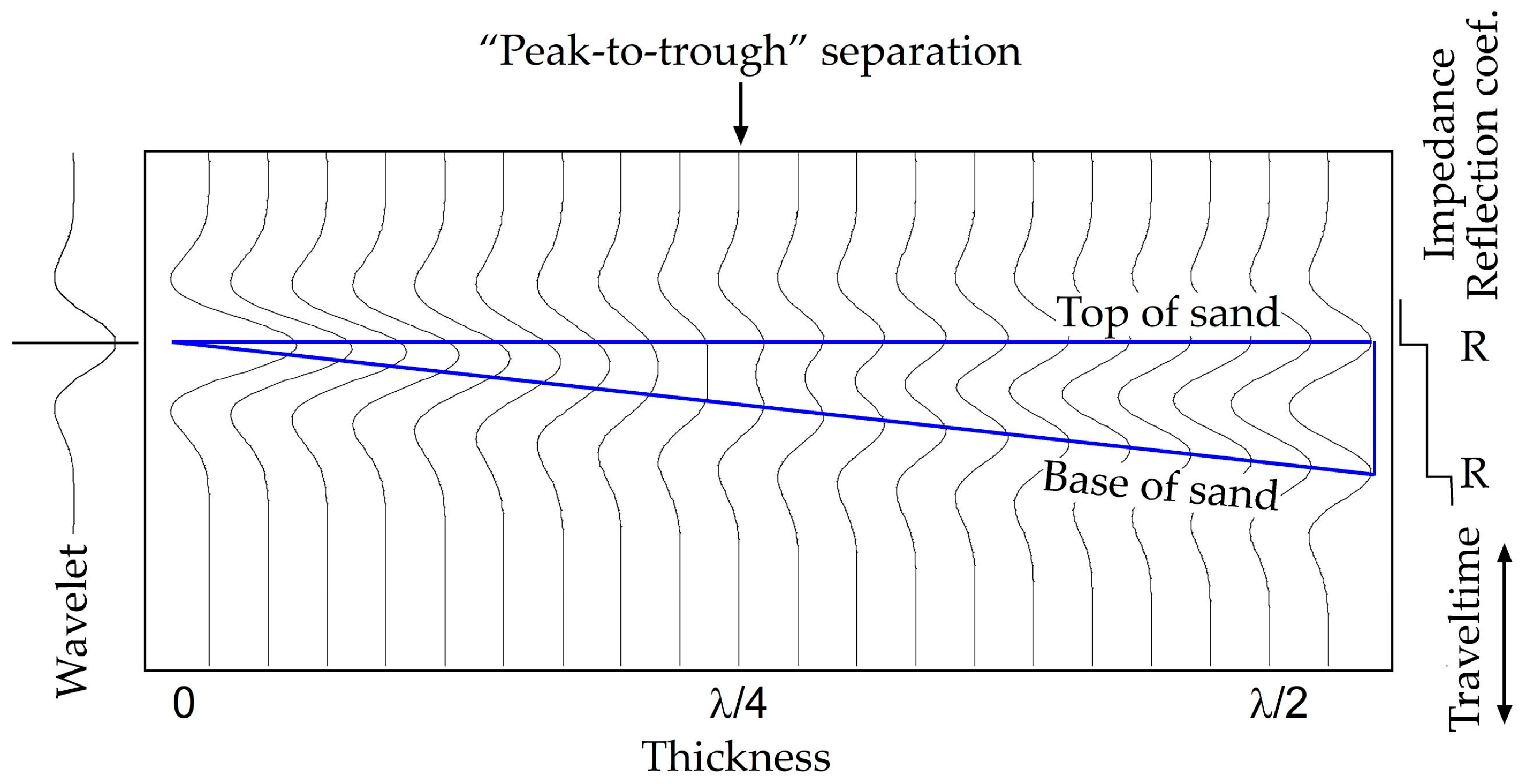
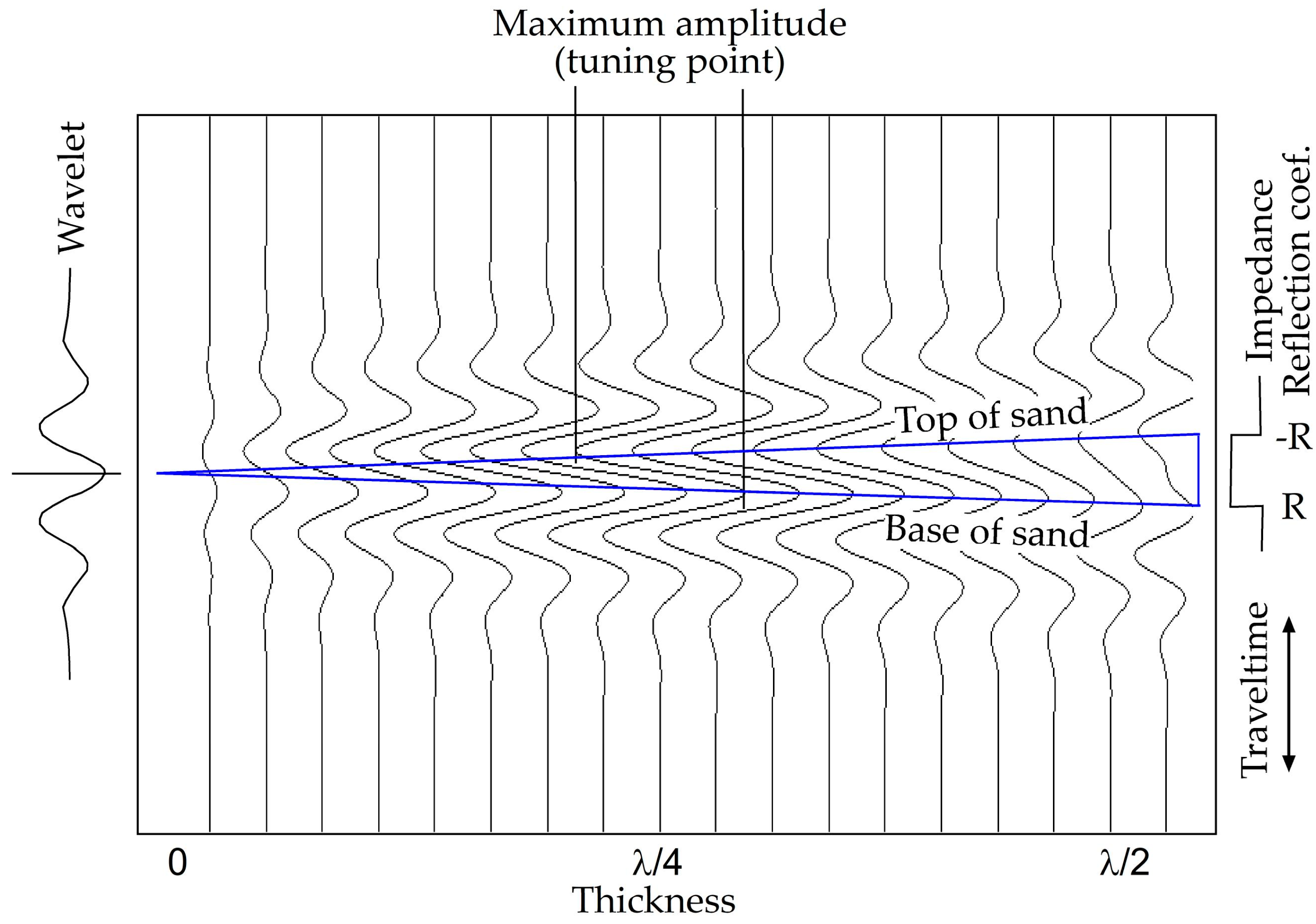
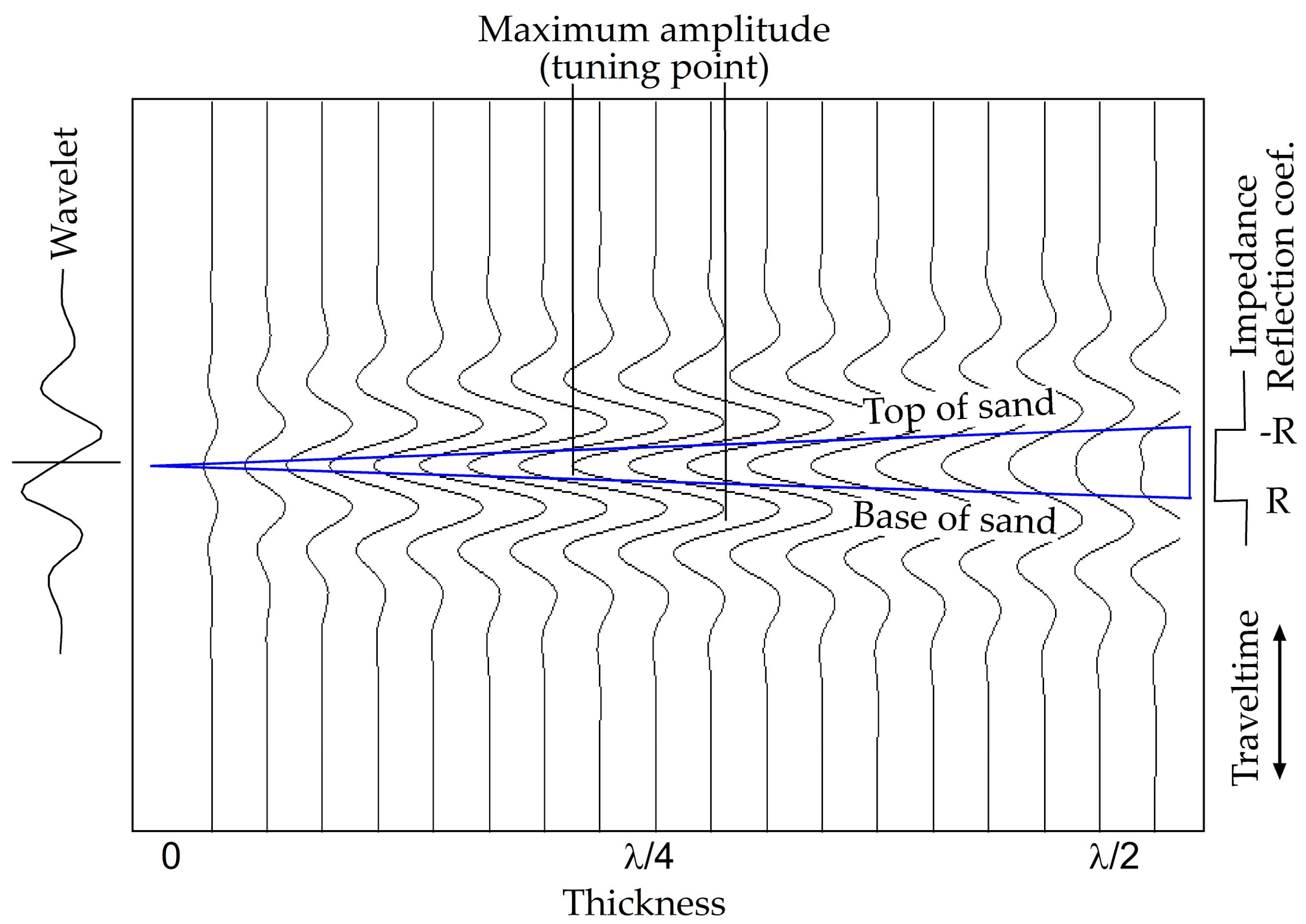
2. Current Understanding of Seismic Resolution

The concept of seismic resolution evolves with time. Three definitions have been established over the past 70 years based on different criteria [13]. Widess [14] argued that the constant “peak-to-trough” propagation time at λ/8 (λ = dominant wavelength typically between 15 and 150 m) is the seismic resolvable limit. Ricker [15] believed that the “flat spot” of the composite waveform at <λ/4 should be defined as the limit of resolvability. Kallweit and Wood’s [16] “peak-to-trough separation” or Rayleigh’s criteria have become widely accepted. They convinced most interpreters that, for a wedge with a step-wise impedance profile (e.g., a moderate-impedance sandstone encased in lower impedance shale above and a higher impedance shale below, see Figure 1), the resolution limit is most practically defined by the “peak-to-trough separation” of the composite waveform at λ/4, where two peaks (point to right) can be identified with a center shallow trough (point to left). For a wedge with a box impedance profile (e.g., a sandstone encased in higher impedance shale), this corresponds to the amplitude “tuning point”, where the maximum composite amplitude is measured (see Figure 2). The concept of resolution is closely tied to our cognitive understanding of the geologic subject (e.g., a feature, a 2D bed, or a 3D body). New concepts may emerge in the future to accommodate new interpretational demands. In addition, the definition of seismic resolution is derived from an idealized earth model and represents the best theoretical resolution. However, the actual resolution is not always as high as the theoretical resolution, partly due to imperfect interpretation. We aim to find more efficient techniques and workflows to improve the actual resolution.

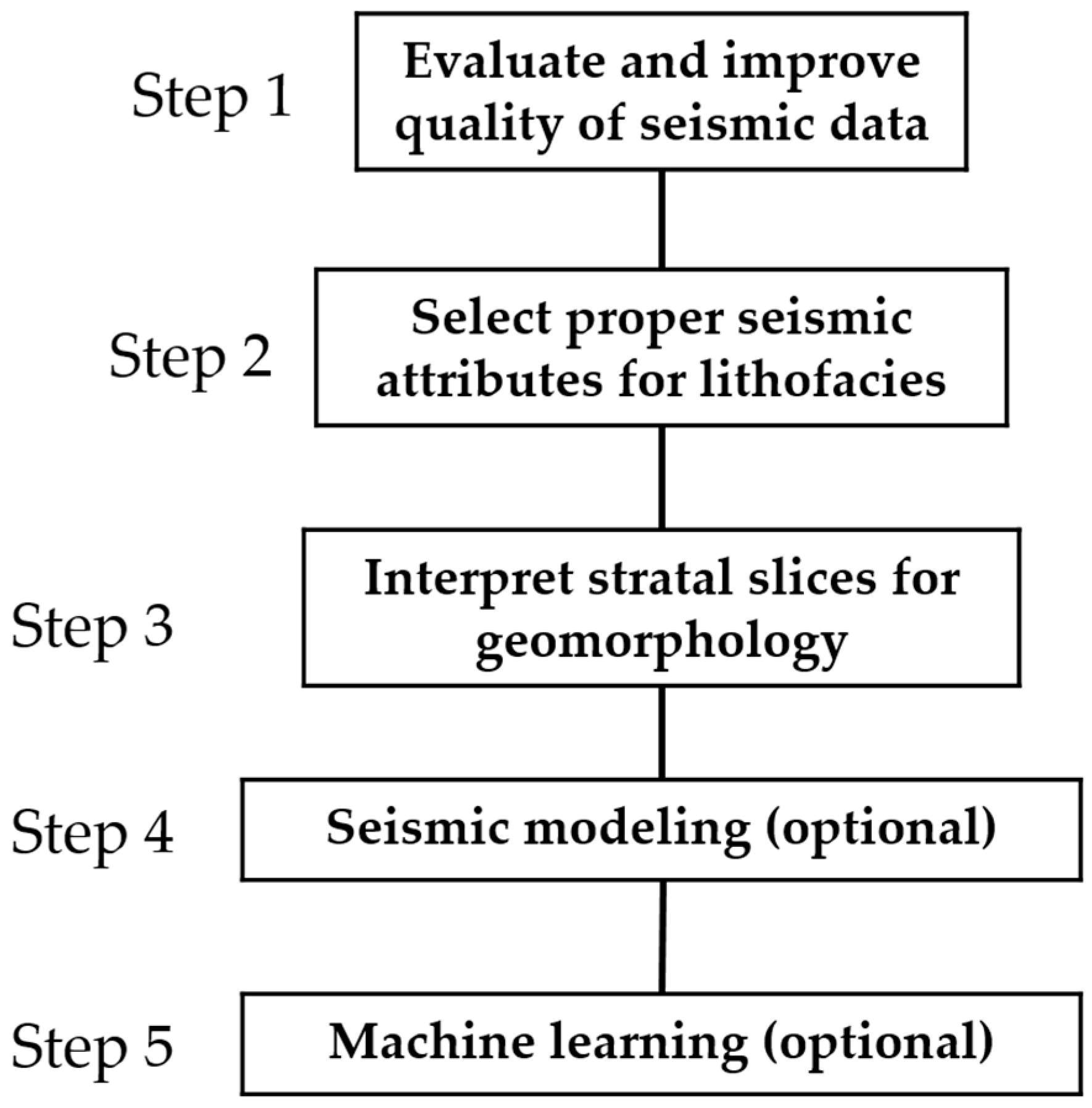
3. Methodology and Workflow

Seismic sedimentology in essence is the combined study of seismic lithology and seismic geomorphology, aimed at high-resolution integration between geological and geophysical information. Converting the seismic waveform to the −90° phase for relative impedance (inversion), frequency fusion, and stratal slicing are key techniques in the current stage [3,10,13]. The results have to be calibrated to core and wireline-log interpretation, and outcrop models wherever available for the best outcome. In light of artificial intelligence, machine learning techniques appear very promising [13].

A workflow for high-resolution subsurface facies and reservoir mapping is proposed in Figure 3. This seismic-sedimentology-guided workflow includes three mandatory steps and two optional steps. The mandatory steps are proven to be key steps by many previous studies (to list a few, [10,12,17,18,19,20]). Optional steps are supported by more recent studies (e.g., [21,22,23,24,25]) and are useful for extra-fine-quality interpretation. The following is a detailed description of each step with application examples where appropriate:

3.1. Step 1: Evaluate and Improve the Quality of Seismic Data

The quality of seismic data is crucial for accurate stratigraphic and sedimentological interpretation. Over the last several decades, academia and the industry have significantly advanced data acquisition and processing. Modern digital subsurface seismic data typically feature a 10 to 100 Hz frequency range, utilize a zero-phase wavelet, maintain precise 3D positioning in migrated data, and possess a satisfactory signal-to-noise ratio. We can still perform various analyses even with imperfect data—such as numerous legacy 3D data sets collected in the 1980s and 1990s. Numerous published case studies of seismic geomorphology and seismic sedimentology from the last thirty years rely on these legacy data sets (e.g., [10,26,27]).

Geologic interpreters can seek assistance from geophysicists to achieve cost-effective improvements in data quality through reprocessing and specialized processing techniques. For example, significant efforts have been made to enhance data processing for higher seismic resolution. A common approach is to extrapolate or to reshape the bandwidth using poststack data, for instance, spectral balancing [28,29], spectral-decomposition-based inversion [30], bandwidth extension [31,32], and pseudo deconvolution using inverse continuous wavelet transform [33].

3.2. Step 2: Select Proper Seismic Attributes for Seismic Lithology

For the processed seismic data available to interpreters, the main aspects influencing actual resolution are choosing attributes, selecting frequency bandwidth, and choosing the wavelet shape. Specific strategies are more effective for geologic and geophysical studies, including stratigraphy, sedimentology, structure, rock physics, or fluid content. A comprehensive understanding of these issues requires an extensive literature review. This section will concentrate specifically on the effective strategies for stratigraphic and sedimentological interpretations.

1. Choice of attributes: A seismic attribute can be any measurement of seismic data. Many seismic attributes can connect seismic signals to a reservoir formation’s acoustic impedance, lithology, and porosity profile. Notable examples include the 90°-phase trace, integrated trace, and model-based inversion, which are all valuable attributes. Currently, seismic trace (waveform) serves as the primary platform for investigation. Based on the author’s experience, the 90°-phase trace is straightforward, geologist-friendly, and preferred (as discussed in the next section). Additionally, some specific attributes known as thin-bed indicators can indicate thin beds at or below seismic resolution. These thin-bed attributes include instantaneous attributes [34], singularity attributes [35,36,37], and phase residues [38]. We hope to see more model and case studies in the near future to promote the widespread application of these attributes in the industry, hoping to reduce the bias of using limited attributes.

2. Wavelet shape and compactness: Zero-phase and 90°-phase waveforms represent two of the most important symmetric waveforms used by seismic interpreters in the petroleum industry. Seismic interpreters often prefer using zero-phase wavelets due to their symmetric waveform, which offers the most compressed representation and the best temporal resolution [39]. However, this advantage mainly applies when analyzing a single reflection surface, such as structural mapping. Suppose the subject is a thin bed (see Figure 2). In that case, the composite waveform centered at the thin bed turns antisymmetric (meaning a main waveform lobe followed an equal amplitude but opposite polarity lobe), removing the benefits of the symmetric wavelet. Researchers can employ a 90° wavelet to recreate a symmetric waveform to address this issue while preserving compactness and optimal resolution [40,41] (see Figure 4).

When comparing a series of stratal slices created with 90° data to those derived from a zero-phase cube within the same strata, interpreters will notice that the 90° slice series displays fewer channel fingerprints [41]. This difference is due to there being less mixing of the vertically stacked reflections, leading to reduced interference. This method is particularly effective for interpreting interbedded thin-bed sequences.

3. Approaches to using frequency information: Frequency components in subsurface seismic data are intrinsically related to bed-thickness distribution in a geologic formation. Seismic frequency analysis and utilization have significantly progressed during the last three decades. Partyka et al. [42] invented the spectral decomposition method, applying the short-window discrete Fourier transform (SWDFT) to calculate the spectral energy for time–frequency cubes. In contrast, Grossmann and Morlet [43] developed the continuous wavelet transform (CWT), which correlated a set of wavelets across a travel time trace to create localized frequency images of the seismic trace in time. This method was refined by matching pursuit decomposition (MPD) to achieve higher vertical resolution in the frequency domain [44,45,46].

Moreover, avoiding mixing low-frequency components with high-frequency subsets in a display can significantly enhance thin-bed resolution. A better approach is the RGB color blending of high-, moderate-, and low-frequency spectral components or seismic travel time traces, also called frequency fusion [22,47]. Notably, when using 90° data, frequency fusion allows for integrating both thick and thin beds in the vertical view. As a result, the typically constant width of seismic events in conventional stacked and migrated color display (Figure 5a) aligns more accurately with the true thickness of lithofacies’ bodies (in this case, sand bodies a through g, Figure 5b) without substantial interference. In the horizontal view, the broken images of channels in the conventional display (#1–#8, Figure 5c) appear more continuous, revealing more realistic, thickness-adjusted channel geometry (Figure 5d).

Additionally, frequency fusion proves advantageous for reconstructing a formation’s sequence-stratigraphic and sedimentological profile in the vertical sectional view. It creates a display illustrating lithofacies and stratigraphic cyclicity, resembling outcrop photos (Figure 6a). In contrast, MPD-processed frequency decomposition in the frequency domain does not achieve the same effect (Figure 6b).

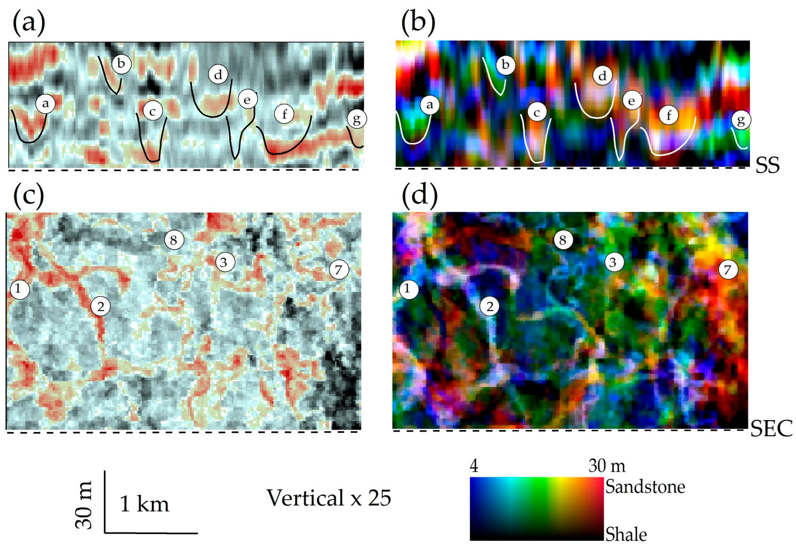
3.3. Step 3: Interpret Stratal Slices for Seismic Geomorphology

If processed correctly, the horizontal resolution of a 3D seismic cube should be roughly equivalent to its vertical resolution [48]. However, the effectiveness of either resolution in seismic investigation is subject to the natural stacking pattern of lithofacies in the geological strata. The proportion of a lithofacies unit’s horizontal to vertical dimensions in the formation controls its spatial resolution status.

From outcrop observations, most thin sedimentary units are prominent in horizontal dimensions (tens to thousands of meters) and minor in vertical dimensions (several meters to low tens of meters). Such thin beds can only be detected in the vertical dimension, although they can be resolved in the horizontal dimension. Thin beds are volumetrically critical in both marine and lacustrine formations. Luckily, many of these beds can be reliably interpreted using seismic geomorphology on stratal slices or horizontal seismic attribute display following depositional surfaces. Therefore, the seismic interpretation of thin beds is limited only to what can be detected.

In a case study [12] (Figure 7), a 50 Hz dominant-frequency data set in a lacustrine basin in China is adjusted to a 90° phase, such that the seismic reflection amplitude indicates lithology: positive (red) amplitudes are associated with sandstones, while negative (black) amplitudes indicate shale. Seismic geomorphic patterns of sandstones are ranked by size and thickness and include channels (distributary sands), irregular sheet-like amplitudes between channels (sandy mixtures formed in marginal environments such as crevasse splays), and random patchy amplitudes (residual sands interspersed in shales, probably formed during transgression). The patterns indicate the presence of two shallow-water deltaic systems originating from the basin’s upper-side (northern) margin. Such deltas are typical of lacustrine shallow-water deltas and are characterized by well-developed straight-to-networked distributary channel systems and poorly developed mouth bars and sand sheets at the delta front. In wells, the thickness of the sandstone in this delta varies from about 0.5 (prodelta) to 10 m (delta plain). It is confirmed with wireline-log verification that distributary channel sands as thin as one meter (λ/80) can be spatially resolved (Figure 7)—much thinner than the λ/25 speculated by Sheriff [49] decades ago.

Seismic geomorphology can be analyzed on time, reflection horizon, and stratal slices [7,50], as long as they are made following geologic-time-equivalent depositional surfaces. Ideally, stratal slices are the preferred option, as they are created by proportional slicing between two reference geologic events (e.g., maximum flooding surfaces) without significant internal depositional hiatuses (e.g., angular unconformities) [7]. Readers are referred to Zeng and Hentz [10] for the relationship between stratal slice and system tracts during deltaic development.

3.4. Step 4: Seismic Modeling (Optional)

Seismic modeling, as suggested by Schlager [9], is essential for establishing a clear connection between seismic lithology, geomorphology, and facies while also identifying potential pitfalls. Unlike the intricate structural and rock-physical models often discussed in the SEAM project of the Society of Exploration Geophysicists, geological and seismic models do not need to be overly complex for many sedimentary interpretations. Simple acoustic and convolutional models, which geologists can create and interpret, are typically sufficient unless otherwise specified. When elastic and wave-equation-guided modeling is required, staff geophysicists can provide critical assistance.

Although modeling is generally case-sensitive and should be tailored to specific geological and geophysical conditions, several important lessons can be easily summarized from simple, convolutional models:

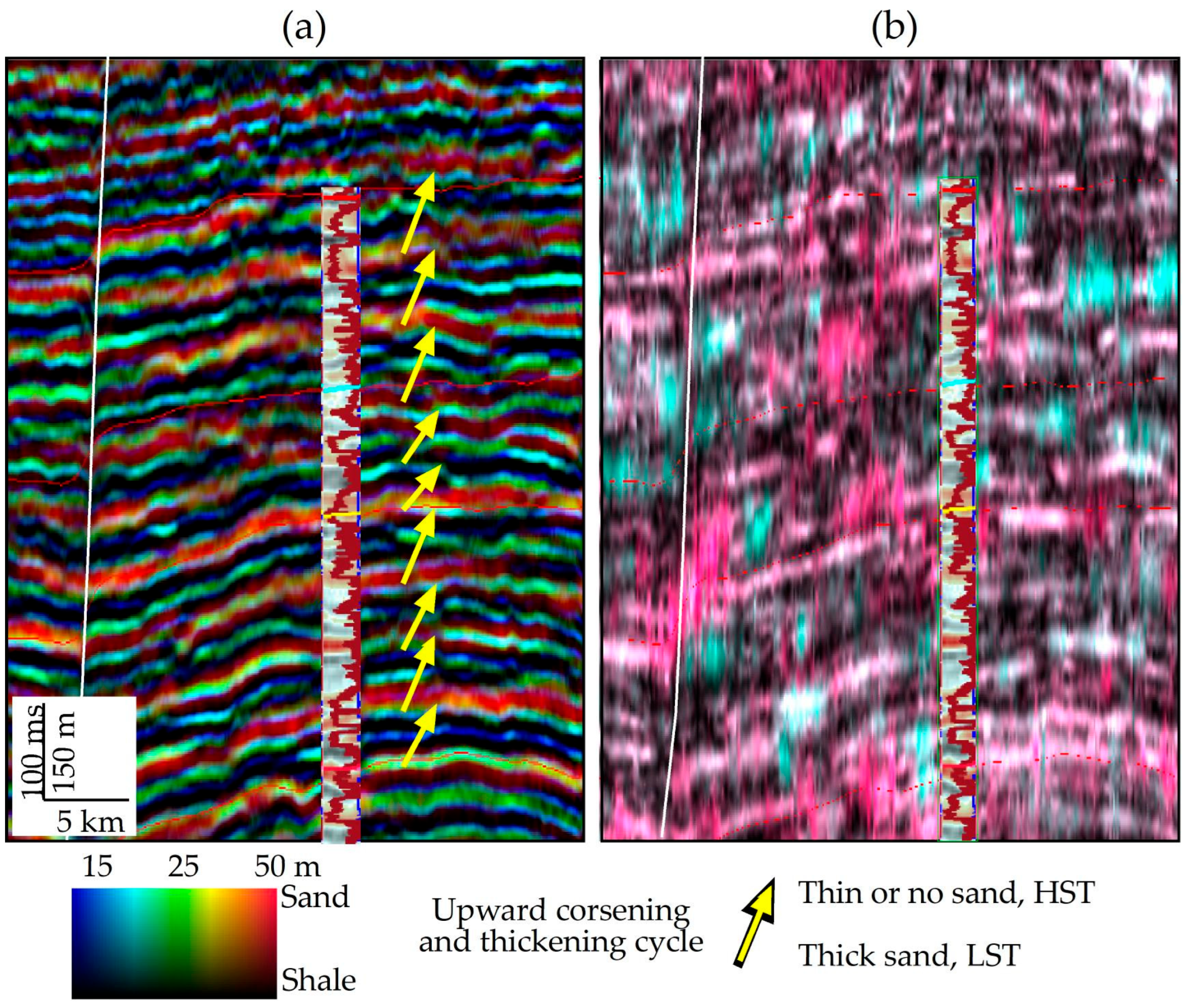
• For a typical, interfingered sand–shale profile, a 90°-phase trace is a reasonable estimation for acoustic impedance and, therefore, for lithofacies (Figure 4);
• Maximum amplitude at λ/4 defines the seismic resolvable limit and, at the same time, illustrates the amplitude tuning phenomenon that is a pitfall to porosity mapping (Figure 3 and Figure 4);
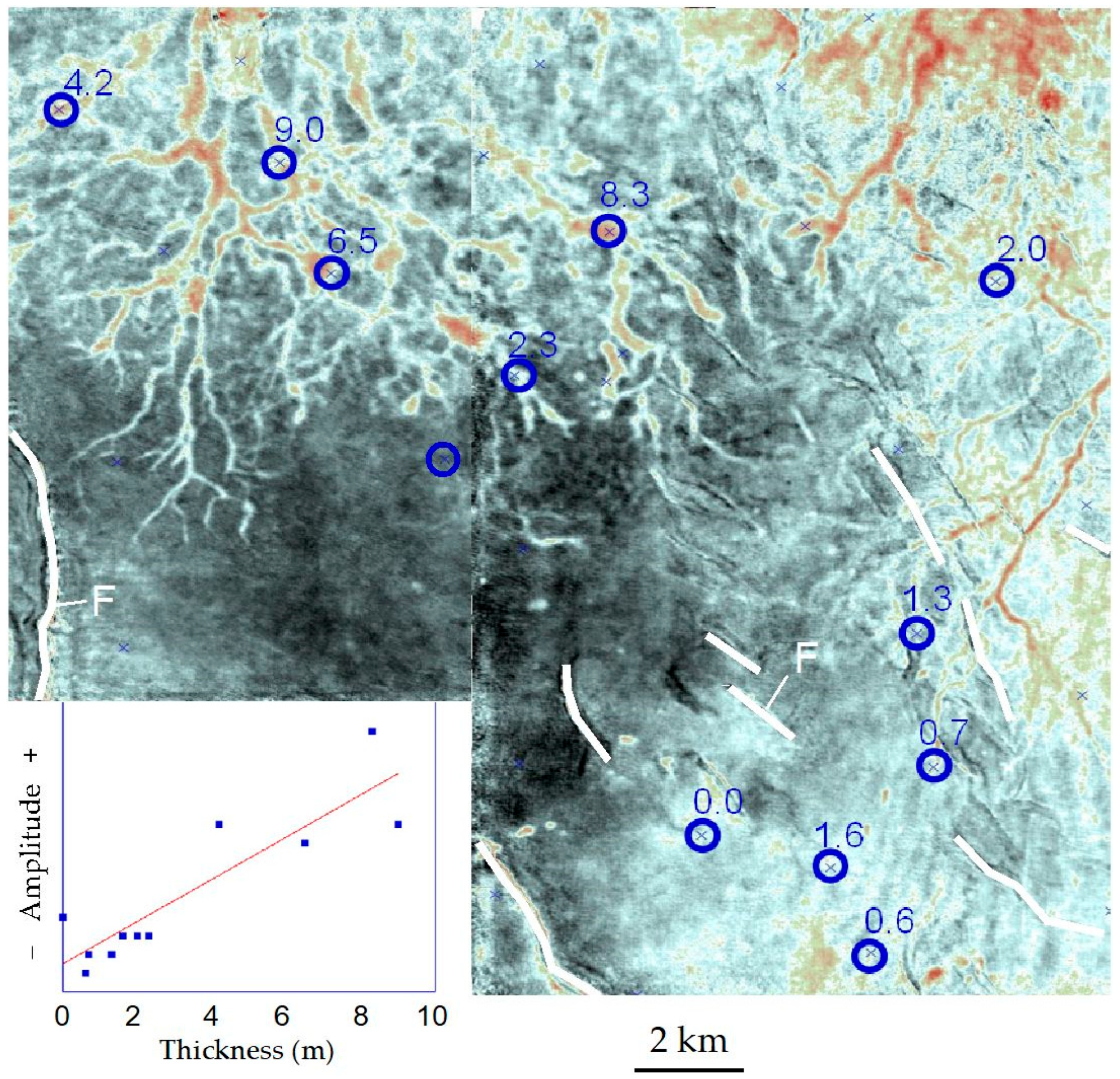
• Seismic onlap or downlap patterns do not necessarily indicate the true pinch-out points of lithofacies [51];
• Seismic reflections do not necessarily follow geologic-time surfaces [7,52,53]; stratal slices are better choices for sedimentary facies imaging [7,54];
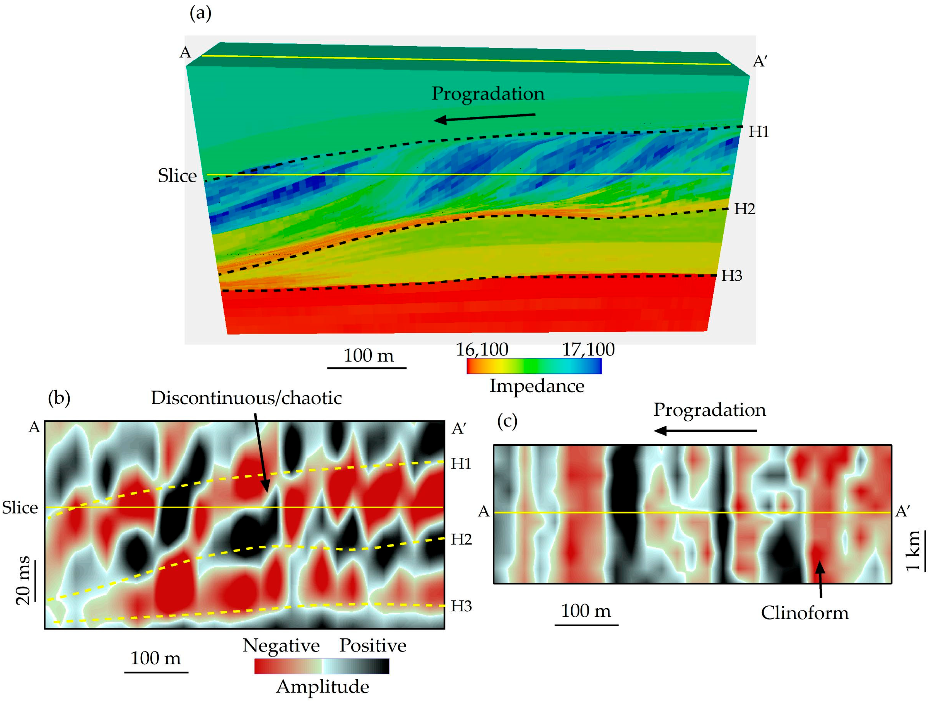
• For a thin and shingled progradational sequence common in shallow-water deltaic systems or prograding carbonate platforms (Figure 8a), seismic clinoforms are challenging to recognize in the vertical section (Figure 8b) but more visible in a horizontal view (Figure 8c), showing the power of horizontal seismic resolution [23].

It should be pointed out that, in practice, no models are complex enough to cover true geologic realities and some simplifications in modeling are always necessary. When making interpretations of seismic models, we should always consider multiple possible scenarios to avoid misleading, over-stretching conclusions.

3.5. Step 5: Machine Learning for Ultrahigh-Resolution Interpretation (Optional)

Machine learning (ML) is becoming increasingly important in various geoscience fields today. It can effectively learn detailed information about core and wireline-log characteristics—specifically the vertical and lateral variations in facies and lithology—by using a quality training data set to predict those characteristics in areas between wells. This process involves a complex nonlinear regrouping of seismic attributes guided by local stratigraphic and sedimentologic models. Model testing has demonstrated the potential of this approach (see Figure 9). For instance, in an interbedded formation (Figure 9a), the band-limited seismic responses (Figure 9b) display rounded bed boundaries and often miss variations in thickness. While ML can utilize single-well training data to predict some thickness variations, the boundaries remain mostly blurred. This trade-off suggests that, although there is improved resolution, some limitations still exist (Figure 9c).

In contrast, a model based on 500 wells conveys much of the high-resolution information in the predicted section, resulting in sharp boundaries (Figure 9d). These two cases illustrate the range of improvements expected in practical AI applications. While more studies are needed to uncover the detailed mechanisms behind these processes, ML is poised to significantly enhance below-seismic-resolution thin-bed mapping using seismic data, creating numerous opportunities for exploring and developing conventional and unconventional resources.

However, we have to agree that the application of machine learning is still in its early stages. Many recent case studies, including this example, are overly simplistic. There are many challenges remaining. For example, the field data, both seismic and well data, are not noise free, and the rock-physics model in the real world is not ideal. Without knowledge of the true impedance model, we could perform only a blind-well test to evaluate the quality of prediction and its practical value. Further research is necessary to build confidence in this technology.

In summary, this five-step workflow is designed for thin beds (thickness < seismic resolvable limit, typically meters to low tens of meters) where the interpretability of a seismic reflection event is governed by the seismic tuning effect. It does not necessarily improve the interpretation of thick reservoirs (high tens of meters or more) when the top and base of the reservoirs can be picked out directly on reflection seismic events. When such thick reservoir beds are involved, conventional approaches (e.g., seismic stratigraphy, instantaneous seismic attributes, etc.) are still effective.

4. Future Improvements

Similarly to any of the subfields of science and technology that were initiated upon challenges being faced in the petroleum industry and which are growing rapidly, seismic geomorphology, and even more so seismic sedimentology, is facing demands for improvement. A few are listed as follows:

1. Better calibration with well and outcrop information and regional/local geologic models: When interpreting seismic data, it is important to understand that interpretation merely approximates the truth and is not necessarily the truth itself. Interpretation is seldom unique and must be verified before finalization. Therefore, we should always verify and calibrate seismic interpretation with well and outcrop observations. For example, in this study, well–seismic calibrations are vital to demonstrate the value of seismic sedimentological approaches. The necessity of using a 90° seismic volume and frequency fusion in seismic stratigraphic profiling is demonstrated by superimposing wireline-log (gamma ray) onto a seismic section (Figure 6); the superhigh spatial resolution of stratal slices is verified by wireline-log-measured sandstone thickness (Figure 7); and the predictive power of machine learning could not be accessed without overlapping well-site impedance logs (Figure 9). In areas without drilling data or which are lacking outcrop analogs, it is advisable to use a geologic model in adjacent regions or comparable formations to enhance the interpretive process. Harishidayat et al. [55] proposed an integrated workflow combining subsurface seismic geomorphology with surface geomorphology to create a reliable 3D model of the Earth and its geomorphological features.

2. Push for deeper integration: How can we leverage current knowledge and technology to enhance seismic sedimentology? There are at least two key approaches to consider. First, we should focus on publishing more geologic models and case histories that validate practical workflows and thin-bed indicative attributes. Increasing the number of models and case studies can improve our understanding of various depositional systems under different data conditions. Moreover, achieving higher resolution is not solely the responsibility of geophysicists; it requires increased collaboration with geologists. To foster this collaboration, we should build highly integrated research and operational teams. Furthermore, we should encourage undergraduate and graduate students in geoscience programs to broaden their curriculum by including a diverse range of geological and geophysical disciplines.

3. Look forward to the future development of high-resolution geophysics: Recent widespread applications of seismic sedimentology have shown tremendous potential for resource exploration and development in various basins, mainly where seismically, thin beds serve as the dominant reservoirs. However, we should realize that under current acquisition and processing technologies, seismic data still have limits in resolution. It is dangerous to claim that current approaches can solve all the problems for thin-bedded reservoirs. Extracting spatial resolution on stratal slices often involves a trade-off with band-limited seismic data. Closely spaced thin beds within the width of a single seismic event, typically ranging from 5 to 40 m (λ/4) in their interval, are challenging to differentiate in both vertical sections and horizontal views, which can lead to confusion. We need next-generation, broad-bandwidth acquisition and processing technologies to tackle the mapping difficulties associated with these thin beds. Some new developments in high-resolution 3D (HR3D) [56,57] are promising in revealing thin-bed geology with a signal of up to 200 Hz at 1 s (1000–1200 m) depth.

5. Conclusions

By reviewing our current understanding of seismic resolution and proposing a workflow for the high-resolution interpretation of depositional facies and reservoirs, I have revealed that the following:

• For lithologic and facies mapping using seismic data, “high-resolution” refers to the ability to interpret the top and base of a sedimentary bed with a thickness of λ/4 (typically between 15 and 150 m) in a vertical view. Additionally, it enables the detection of beds as thin as λ/80, which range from 1 to 5 m when applying seismic sedimentology from a horizontal perspective.
• Displaying 90° data and frequency fusion on a stratal slice is one of the most effective thin-bed detective workflows for seismic sedimentology among various attribute and visualization format choices.
• Seismic modeling is essential for verifying and calibrating seismic sedimentological interpretations, such as defining seismic resolution and the true link between reflection configurations and local stratal and sedimentary architectures.
• Machine-learning-based approaches can offer a more accurate interpretation of thin-bed seismic sedimentology.

References

1. Vail, P.R.; Mitchum, R.M., Jr.; Thompson, S., III. Stratigraphic interpretation of seismic reflection patterns in depositional sequences. In Seismic Stratigraphy; Payton, C.E., Ed.; American Association of Petroleum Geologists Memoir: Tulsa, OK, USA, 1977; Volume 26, pp. 63–82. [Google Scholar]
2. Chopra, S.; Marfurt, K. Seismic attributes for prospect identification and reservoir characterization. Soc. Explor. Geophys. Geophys. Dev. Ser. 2007, 11, 464. [Google Scholar]
3. Zhu, X.; Dong, Y.; Zeng, H.; Lin, C.; Zhang, X. Current status and future of seismic sedimentology in China. J. Palaeogeogr. 2020, 22, 397–411. [Google Scholar]
4. Posamentier, H.W. Seismic geomorphology and depositional systems of deep-water environments: Observations from offshore Nigeria, Gulf of Mexico, and Indonesia. In Proceedings of the 64th EAGE Conference & Exhibition, Florence, Italy, 27–30 May 2002. [Google Scholar] [CrossRef]
5. Posamentier, H.W. Seismic Geomorphology: Imaging Elements of Depositional Systems from Shelf to Deep Basin Using 3D Seismic Data: Implications for Exploration and Development. Geol. Soc. Lond. Mem. 2004, 29, 11–24. [Google Scholar] [CrossRef]
6. Posamentier, H.W. Application of 3D seismic visualization techniques for seismic stratigraphy, seismic geomorphology, and depositional systems analysis: Examples from fluvial to deep-marine depositional environments. Geol. Soc. Lond. Pet. Geol. Conf. Ser. 2005, 6, 1565–1576. [Google Scholar] [CrossRef]
7. Zeng, H.; Henry, S.C.; Riola, J.P. Stratal slicing: Part II. Real seismic data. Geophysics 1998, 63, 514–522. [Google Scholar] [CrossRef]
8. Johnston, D.H. (Ed.) Methods and applications in reservoir geophysics. In Society of Exploration Geophysicists Investigations in Geophysics Series 15; Society of Exploration Geophysicists: Tulsa, OK, USA, 2010. [Google Scholar]
9. Schlager, W. The future of applied sedimentary geology. J. Sediment. Res. 2000, 70, 2–9. [Google Scholar] [CrossRef]
10. Zeng, H.; Hentz, T.F. High-frequency sequence stratigraphy from seismic sedimentology: Applied to Miocene, Vermilion Block 50, Tiger Shoal area, offshore Louisiana. Am. Assoc. Pet. Geol. Bull. 2004, 88, 153–174. [Google Scholar] [CrossRef]
11. Lutome, M.S.; Lin, C.; Chunmei, D.; Zhang, X.; Harishidayat, D. Seismic sedimentology of lacustrine delta-fed turbidite systems: Implications for paleoenvironment reconstruction and reservoir prediction. Mar. Pet. Geol. 2020, 113, 104159. [Google Scholar] [CrossRef]
12. Zeng, H. Ultra-thin, lacustrine sandstones imaged on stratal slices in the Cretaceous Qijia Depression, Songliao Basin, China. In Proceedings of the Society of Exploration Geophysicists Annual Meeting, San Antonio, TX, USA, 18–23 September 2011; pp. 951–955. [Google Scholar]
13. Zeng, H. Improving the resolution of 3-D seismic data. Explor. Am. Assoc. Pet. Geol. 2024, 45, 44–47. [Google Scholar]
14. Widess, M.B. How thin is a thin bed? Geophysics 1973, 38, 1176–1180. [Google Scholar] [CrossRef]
15. Ricker, N. Wavelet contraction, wavelet expansion and the control of seismic resolution. Geophysics 1953, 18, 769–792. [Google Scholar] [CrossRef]
16. Kallweit, R.S.; Wood, L.C. The limits of resolution of zero-phase wavelets. Geophysics 1982, 47, 1035–1046. [Google Scholar] [CrossRef]
17. Carter, D.C. 3-D seismic geomorphology: Insights into fluvial reservoir deposition and performance, Widuri field, Java Sea. Am. Assoc. Pet. Geol. Bull. 2003, 87, 909–934. [Google Scholar] [CrossRef]
18. Zhao, W.; Zou, C.; Chi, Y.; Zeng, H. Sequence stratigraphy, seismic sedimentology, and lithostratigraphic plays: Upper Cretaceous, Sifangtuozi area, southwest Songliao Basin, China. Am. Assoc. Pet. Geol. Bull. 2011, 95, 241–265. [Google Scholar] [CrossRef]
19. Van Dyke, S.K. Stratal slicing for seismic sedimentology. Int. Basic Appl. Res. J. 2015, 1, 1–6. [Google Scholar]
20. Cheng, S.; Jiang, Y.; Li, J.; Li, C.; Xu, L. Reservoir prediction in a development area with a high-density well pattern using seismic sedimentology: An example from the BB2 block, Changyuan LMD oil field, Songliao Basin, China. Interpretation 2015, 3, SS87–SS99. [Google Scholar] [CrossRef]
21. Zhang, G.; Wang, Z.; Chen, Y. Deep learning for seismic lithology prediction. Geophys. J. Int. 2018, 215, 1368–1387. [Google Scholar] [CrossRef]
22. Yue, D.; Li, W.; Wang, W.; HU, G.; Qiao, H.; Zhang, M.; Wang, W.F. Fused spectral-decomposition seismic attributes and forward seismic modeling to predict sand bodies in meandering fluvial reservoirs. Mar. Pet. Geol. 2019, 99, 27–44. [Google Scholar] [CrossRef]
23. Zeng, H.; Xu, Z.; Liu, W.; Janson, X.; Fu, Q. Seismic-informed carbonate shelf-to-basin transition in deeply buried Cambrian strata, Tarim Basin, China. Mar. Pet. Geol. 2022, 136, 18. [Google Scholar] [CrossRef]
24. Li, W.; Yue, D.; Colombera, L.; Duan, D.; Long, T.; Wu, S.; Liu, Y. A novel method for seismic-attribute optimization driven by forward modeling and machine learning in the prediction of fluvial reservoirs. Geoenergy Sci. Eng. 2023, 227, 211952. [Google Scholar] [CrossRef]
25. Xu, Z.; Li, J.T.; Li, J.; Yan, C.; Yang, S.; Wang, Y.; Shao, Z. Application of 9-component S-wave 3D seismic data to study sedimentary facies and reservoirs in a biogas-bearing area: A case study on the Pleistocene Qigequan Formation in Taidong area, Sanhu Depression, Qaidam Basin, NW China. Pet. Explor. Dev. 2024, 51, 647–660. [Google Scholar] [CrossRef]
26. Posamentier, H.W. Ancient shelf ridges—A potentially significant component of the transgressive systems tract: A case study from offshore northwest Java. Am. Assoc. Pet. Geol. Bull. 2002, 86, 75–106. [Google Scholar]
27. Dong, Y.; Zhu, X.; Zeng, H.; Bian, S.; Liu, C.; Cheng, K.; Xu, X. Study of seismic sedimentology in Qinan Sag (China). J. China Univ. Pet. 2008, 32, 7–12. [Google Scholar]
28. Fehmers, G.C.; Höcker, C.F.W. Fast structural interpretation with structure-oriented filtering. Geophysics 2003, 68, 1286–1293. [Google Scholar] [CrossRef]
29. Chopra, S.; Marfurt, K. Spectral decomposition and spectral balancing of seismic data. Lead. Edge 2016, 25, 176–179. [Google Scholar] [CrossRef]
30. Portniaguine, O.; Castagna, J.P. Inverse spectral decomposition. In Proceedings of the 74th Annual International Meeting, Society of Exploration Geophysicists, Expanded Abstracts, Denver, CO, USA, 10–15 October 2004; pp. 1786–1789. [Google Scholar]
31. Smith, M.G.P.; Stein, J.; Bertrand, A.; Yu, G. Extending seismic bandwidth using the continuous wavelet transform. First Break 2008, 26, 97–102. [Google Scholar] [CrossRef]
32. Liang, C.; Castagna, J.; Torres, R.Z. Tutorial: Spectral bandwidth extension—Invention versus harmonic extrapolation. Geophysics 2017, 82, W1–W16. [Google Scholar] [CrossRef]
33. Matos, M.C.; Marfurt, K.J. Inverse continuous wavelet transform “deconvolution”. In Proceedings of the 81st Annual International Meeting, Society of Exploration Geophysicists, Expanded Abstracts, San Antonio, TX, USA, 18–24 September 2011; pp. 1861–1865. [Google Scholar]
34. Taner, M.T.; Sheriff, R.E. Application of amplitude, frequency, and other attributes to stratigraphic and hydrocarbon determination. In Seismic Stratigraphy; Payton, C.E., Ed.; American Association of Petroleum Geologists Memoir: Tulsa, OK, USA, 1977; Volume 26, pp. 301–328. [Google Scholar]
35. Liner, C.L.; Li, C.; Gersztenkorn, A.; Smythe, J. SPICE: A new general seismic attribute. In Proceedings of the 74th Annual International Meeting, Society of Exploration Geophysicists, Expanded Abstracts, Denver, CO, USA, 10–15 October 2004; pp. 433–436. [Google Scholar]
36. Li, C.; Liner, C. Singularity exponent from wavelet-based multiscale analysis: A new seismic attribute. Chin. J. Geophys. 2005, 48, 953–959. [Google Scholar] [CrossRef]
37. Li, C.; Liner, C. Wavelet-based detection of singularities in acoustic impedances from surface seismic reflection data. Geophysics 2008, 73, V1–V9. [Google Scholar] [CrossRef]
38. Matos, M.C.; Davogustto, O.; Zhang, K.; Marfurt, K.J. Detecting stratigraphic discontinuities using time-frequency seismic phase residues. Geophysics 2011, 76, 1–10. [Google Scholar] [CrossRef]
39. Brown, A.R. Interpretation of three-dimensional seismic data. In American Association of Petroleum Geologists Memoir 42, 3rd ed.; Society of Exploration Geophysicists and American Association of Petroleum Geologists: Houston, TX, USA, 1991; p. 341. [Google Scholar]
40. Sicking, C.J. Windowing and estimation variance in deconvolution. Geophysics 1982, 47, 1022–1034. [Google Scholar] [CrossRef]
41. Zeng, H.; Backus, M.M. Interpretive advantages of 90°-phase wavelets: Part 2―Seismic applications. Geophysics 2005, 70, C17–C24. [Google Scholar] [CrossRef]
42. Partyka, G.; Gridley, J.; Lopez, J. Interpretational applications of spectral decomposition in reservoir characterization. Lead. Edge 1999, 18, 353–360. [Google Scholar] [CrossRef]
43. Grossmann, A.; Morlet, J. Decomposition of Hardy functions into square integrable wavelets of constant shape. SIAM J. Math. Anal. 1984, 15, 723–736. [Google Scholar] [CrossRef]
44. Mallat, S.; Zhang, Z. Matching pursuits with time-frequency dictionaries. IEEE Trans. Signal Process. 1993, 41, 3397–3415. [Google Scholar] [CrossRef]
45. Castagna, J.P.; Sun, S. Comparison of spectral decomposition methods. First Break 2006, 24, 75–79. [Google Scholar] [CrossRef]
46. Wang, C.; Zong, Z.; Yin, X.; Li, K. Seismic resolution enhancement with variational modal-based fast-matching pursuit decomposition. Interpretation 2024, 12, T77–T86. [Google Scholar] [CrossRef]
47. Zeng, H. Thickness imaging for high-resolution stratigraphic interpretation by linear combination and color blending of multiple-frequency panels. Interpretation 2017, 5, T411–T422. [Google Scholar] [CrossRef]
48. Lindsey, J.P. The Fresnel zone and its interpretive significance. Lead. Edge 1989, 8, 33–39. [Google Scholar] [CrossRef]
49. Sheriff, R.E. Encyclopedic Dictionary of Exploration Geophysics, 3rd ed.; Society of Exploration Geophysicists: Tulisan, Brazil, 1991; p. 383. [Google Scholar]
50. Posamentier, H.W.; Dorn, G.A.; Cole, M.J.; Beierle, C.W.; Ross, S.P. Imaging elements of depositional systems with 3-D seismic data: A case study. In Proceedings of the Gulf Coast Section SEPM Foundation, 17th Annual Research Conference, Houston, TX, USA, 8–11 December 1996; pp. 213–228. [Google Scholar]
51. Biddle, K.T.; Schlager, W.; Rudolph, K.W.; Bush, T.L. Seismic model of a progradational carbonate platform, Picco di Vallandro, the Dolomites, Northern Italy. Am. Assoc. Pet. Geol. Bull. 1992, 76, 14–30. [Google Scholar]
52. Tipper, J.C. Do seismic reflections necessarily have chronostratigraphic significance? Geol. Mag. 1993, 130, 47–55. [Google Scholar] [CrossRef]
53. He, Y.; Zeng, H.; Kerans, C.; Hardage, B.A. Seismic chronostratigraphy at reservoir scale: Statistical modeling. Interpretation 2015, 3, SN69–SN87. [Google Scholar] [CrossRef]
54. Wang, W.; Wu, X.; Zeng, H.; Janson, X.; Kerans, C. Stratal surfaces honoring seismic structures and interpreted geologic time surfaces. Geophysics 2024, 89, N45–N57. [Google Scholar] [CrossRef]
55. Harishidayat, D.; Al-Shuhail, A.; Randazzo, G.; Lanza, S.; Muzirafuti, A. Reconstruction of Land and Marine Features by Seismic and Surface Geomorphology Techniques. Appl. Sci. 2022, 12, 9611. [Google Scholar] [CrossRef]
56. Kluesner, J.W.; Brothers, D. Seismic attribute detection of faults and fluid pathways within an active strike-slip shear zone: New insights from high-resolution 3D P-CableTM seismic data along the Hosgri fault, offshore California. Interpretation 2016, 4, SB131–SB148. [Google Scholar] [CrossRef]
57. Feng, Y.E.; Meckel, T.; Hess, T. Processing techniques and challenges for high-resolution 3D marine seismic data: Case studies from the Gulf of Mexico and Japan. In Proceedings of the 89th Annual International Meeting, Society of Exploration Geophysicists, Expanded Abstracts, San Antonio, TX, USA, 15–20 September 2019; p. 3969. [Google Scholar]
Figure 1. The seismic resolution as defined in a synthetic model that depicts a step-wise impedance profile of a sand wedge surrounded by lower impedance shale above and higher impedance shale below. A zero-phase Ricker wavelet is used. R refers to the reflection coefficient. In this case, Kallweit and Wood’s [16] “peak-to-trough separation” at λ/4 is accepted as a seismic resolvable limit.
Applsci 15 06387 g001
Figure 2. At λ/4 thickness, maximum amplitude (tuning point) is observed in a synthetic model of a low-impedance wedge (sand) encased in high-impedance rock (shale). A zero-phase wavelet is applied. R refers to the reflection coefficient. The thickness at the tuning point is equivalent to the seismic resolvable limit.
Applsci 15 06387 g002
Figure 3. Proposed workflow for high-resolution, subsurface sedimentary facies and reservoir prediction using seismic data.
Applsci 15 06387 g003
Figure 4. The result of the 90°-phase shift in the synthetic model in Figure 2 indicates lithofacies. The central trough is a reasonable estimate of the low-impedance wedge sand lithofacies. Except for the bed which is thinner than λ/8, the top and base of the wedge are tied to the zero-crossings of seismic traces.
Applsci 15 06387 g004
Figure 5. Frequent fusion can further improve the interpretability of 90°-phase data. (a) On a vertical section (labeled SEC) of stacked and migrated data, seismic events (a–g) do not fit the geometry of channel sand bodies. (b) In the same section, using frequency-fused data, RGB events (a–g) roughly fit the geometry of channel sand bodies. (c) On a stratal slice (labeled SS) imaged with stacked and migrated data, channel images (1–8) are mostly blurred. (d) On the same stratal slice with frequency-fused data, channel images (1–8) are more continuous with sharper boundaries and valid thickness definitions.
Applsci 15 06387 g005
Figure 6. High-resolution stratigraphic imaging and analysis are achieved by fusing three frequencies from a 90° seismic volume. (a) System tracts and sequence stratigraphy influenced sand thickness (ranging from 15 to 50 m in the gamma ray log at the well) and depositional cycles [10]. The left deflection of the log indicates sand. (b) An RGB blending of 14, 30, and 50 Hz iso-frequencies created with MPD is not optimal for stratigraphic imaging. Modified from Zeng [13].
Applsci 15 06387 g006
Figure 7. An optimal spatial resolution (1 m) is indicated by a stratal slice created from a 50 Hz dominant-frequency 3D volume in a lacustrine shallow-water deltaic system. The thickness (m) of sandstone measured in gamma ray logs in wells shows a linear relationship with seismic reflection amplitude. Modified from Zeng [12].
Applsci 15 06387 g007
Figure 8. Thin progradational clinoforms show a discontinuous–chaotic vertical pattern but a clear parallel horizontal pattern. (a) A 3D impedance model of an outcrop-based, 50 ms (150 m) thick, progradational sequence. (b) A vertical synthetic seismic section of a 28 Hz wavelet illustrates mostly discontinuous to chaotic reflections. (c) A horizontal amplitude slice showing a parallel pattern perpendicular to the progradation direction. Modified from Zeng et al. [23].
Applsci 15 06387 g008
Figure 9. This is a test of an ML-based inversion workflow. (a) The true model represents the realistic acoustic impedance (Ip) of an interbedded sandstone and shale formation. (b) A 60 Hz Ricker wavelet with a phase shift of 90° is generated from the true model shown in part (a). However, this display omits thickness information. (c) The testing results using a large training data set from a single well achieve the limited recovery of the true thickness variation. (d) In contrast, testing results using a large synthetic training data set composed of 500 wells are able to recover most of the high-resolution details shown in part (a). The logs from the three wells are used solely for blind testing purposes. Modified from Zeng [13].
Applsci 15 06387 g009
Disclaimer/Publisher’s Note: The statements, opinions and data contained in all publications are solely those of the individual author(s) and contributor(s) and not of MDPI and/or the editor(s). MDPI and/or the editor(s) disclaim responsibility for any injury to people or property resulting from any ideas, methods, instructions or products referred to in the content.