Three-Dimensional Pedalling Kinematics Analysis Through the Development of a New Marker Protocol Specific to Cycling

Featured Application

The proposed work will allow us to perform experimental measurements of the 3D kinematics of cyclists in an accurate and efficient way, being the obtained results of interest, especially in the clinical and preventive field.

Abstract

This study aims to develop and evaluate a cycling-specific marker protocol that minimises the number of markers while accounting for the unique biomechanics of cycling. Although movements in the frontal and transverse planes during cycling are limited, they are clinically relevant due to their association with overuse injuries. Existing gait-based marker protocols often fail to consider cycling-specific factors such as posture, range of motion, marker occlusion, and muscle-induced artifacts. The proposed protocol (PP) uses 15 physical and 8 virtual markers. In the absence of a gold standard for 3D pedalling kinematics, the PP was evaluated by comparing it with established gait analysis protocols. The protocol demonstrated high correlation in gait (CCC > 0.98 for hip and knee in the sagittal plane), low intra-subject variability (CV < 15% for hip, knee, and ankle), and high repeatability. During pedalling, position, velocity, and acceleration were measured in all three spatial directions. Notably, angular velocity and linear acceleration showed significant components outside the sagittal plane, particularly for angular velocity. These findings highlight the importance of considering 3D motion when estimating forces, joint moments, and joint-specific powers in cycling biomechanics.

1. Introduction

Kinematic analysis in cycling is a line of research widely developed in the literature due to its applications at the clinical (e.g., rehabilitation treatments) and sports (e.g., performance optimisation) levels. Different types of technology have been used in the literature for kinematic recording of cycling: goniometers [1], video captures [2], LEDs [3], inertial sensors [4] and videogrammetry [5]. Videogrammetry [5] is currently the most widely accepted by the scientific community.

Most kinematic analyses in cycling are focused on the lower body because of its relevance in the development of this task [5,6,7,8,9,10,11,12,13,14,15,16,17]. Most of the pedalling analyses are focused only on the sagittal plane, such as those performed by Bini et al. [6,7], because this plane contains greater ROM. Outside this plane, the results are very sensitive to possible errors due to marker placement or alterations in the trajectory of the markers due to a soft tissue artefact (STA) [18]. However, movements outside the sagittal plane are important from a clinical point of view, as they are the main cause of possible joint overload, pain or injury [13,19,20,21,22].

To increase the reliability of the kinematic results, it is necessary to define a protocol adapted to the activity to be analysed. To the best of our knowledge, all the analysed articles use marker protocols designed for gait analysis. However, these protocols have some drawbacks when analysing a specific activity like cycling.

There are two main drawbacks. First, the existing protocols often use markers that are hidden by the cyclist’s posture. For example, markers placed on the anterior superior iliac spine are often partially or completely hidden when the participant is positioned on the bicycle [5,8,9,10,11,12,13,14,15,16,17]. Second, it is common to place markers in areas where large muscle contractions occur, for example, in the thigh and calf areas. Pedalling can provoke a much higher level of activation in these areas than walking does, resulting in more pronounced muscular contractions and STA. Consequently, the trajectory of markers placed in these areas may change, affecting the results, particularly for those with a small ROM (movements outside the sagittal plane).

Some studies [3,9,11,12,13,14,15,16] have obtained the kinematics by implementing the Least-Square Pose Estimators [23] methodology. This approach is widely used in gait analysis. It is based on the use of a redundant number of markers, with the aim of reducing the effect of STA or loss of marker trajectory. But marker protocols designed with this methodology use a large number of markers, which can affect participant comfort and natural movement during the pedalling test.

An alternative to this type of protocols is the use of nonoptimal pose estimators based on a minimum number of physical markers [23]. Papers in the literature [8] that calculate 3D cycling kinematics tend to use the Plug-in-Gait (PiG) [24] marker protocol. Although this protocol does not affect the comfort of the participants, its characteristics have a high impact on the results obtained [23]. This protocol places markers in the anterior superior iliac spines and in the adipose areas of the thighs and calves [24], areas that are highly affected when the subject pedals. This fact, along with the use of a minimum number of markers, means that the results in cycling using the PiG are highly affected by the placement of the markers, which means that it is not recommendable to use this protocol for the 3D cycling analysis.

This limitation is addressed in the study conducted by Hébert-Losier et al. [12]. In their work, a protocol based on Least-Squares Pose Estimators, utilising 46 markers, was employed. These markers included, among others, those positioned on the anterior superior iliac spines, as well as on the adipose regions of the thighs and legs. All markers were used during static capture; however, for dynamic capture, 14 markers were excluded, including those located on both anterior superior iliac spines. The markers on the thighs and legs were retained, as they constitute a rigid cluster of four markers [12]. The authors treated the 14 excluded markers as technical markers when defining movement, a methodology commonly adopted in gait analysis. The placement of these technical markers is dependent on the physical markers and, consequently, on any associated artefacts or phenomena that may affect them. This approach in cycling research integrates the primary advantages of the two methodologies—Least-Squares Pose Estimators and non-optimal pose estimators. Specifically, it enhances participant comfort during testing, minimises marker trajectory loss, and reduces the sensitivity of the results to marker placement.

The above-discussed aspects motivate the following questions. First: Can a minimised-marker protocol estimate the 3D kinematics in cycling with enough accuracy and repeatability? The next objective was established to answer this question: the development and evaluation of a new marker protocol based on the use of nonoptimal pose estimators, specific for cycling kinematic analysis. The PP will aim to be efficient by avoiding the use of technical reference systems and subsequent transformations to anatomical systems. Furthermore, it shall be based on a minimum number of markers. This helps to minimise the preparation time of the participant by defining a marker placement at points that avoid concealment or artefacts due to the movement of soft masses.

Second: What is the magnitude of non-sagittal kinematics during pedalling at position, velocity and acceleration levels? A 3D kinematic analysis of the lower body during pedalling will be performed to analyse the importance of the three-dimensional character of cycling kinematics. It is well known that the main movement during pedalling is contained in the sagittal plane. However, an analysis of whether the components occurring outside this plane can be neglected or can have an important effect at the dynamic level is intended.

2. Materials and Methods

2.1. Participants

To achieve the objectives established in this study, 19 participants were analysed, all men, adults, with a mean age of 26.87 ± 4.97 years, a mean height of 1.76 ± 0.11 m, a mean weight of 69.56 ± 9.65 kg and a mean BMI of 22.47 ± 2.76 kg/m². The participants were volunteers and reported that they used the bicycle as a means of transport, without seeking to improve their sport or performance. The sample size was based on previous studies found in the literature [25]. The inclusion criteria were as follows:

Inclusion criteria:

• Participants aged 18 years or older.
• Leg length discrepancy (dysmetria) less than or equal to 5 mm.
• Body size compatible with the test bicycle.
• Intrinsic Q-factor similar to the standard Q-factor of the bicycle.

Exclusion criteria:

• Diagnosed locomotor or cardiopulmonary conditions that could interfere with test performance.
• High-performance or professional cyclists.

To assess the discrepancy between lower limbs, each lower limb was measured using the methodology developed by Davis et al. [24]. The participants signed a consent form approved by the Andalusian Biomedical Research Ethics Platform (code number 0230-N-22).

2.2. Instrumentation

A motion analysis system consisting of 12 infrared cameras (100 Hz; Vicon Motion Analysis Inc., Oxford, UK) and 14 mm diameter reflective markers was used. Six of the twelve infrared cameras used were MXT010 models. These are digital cameras with high resolution and a maximum sampling rate of 250 Hz. These cameras, due to their larger size, tended to be positioned higher up (3 m above the ground) and further away from the working volume (2.5–3 m). The remaining six infrared cameras were Bonita models. The cameras were also high-resolution digital cameras and, in this case, the maximum sampling rate was 100 Hz. These cameras, due to their more compact size, were positioned on tripods at the ground level and closer to the participant (1.5 m approximated). The infrared camera models had different maximum sampling frequencies; therefore, when adjusting the equipment, the sampling frequency was set to the lower of the two, in this case, 100 Hz. All data from the twelve infrared cameras were synchronised via a central console called Giganet from the company Vicon^®. This central console also had the function of sending all the data from the recordings to the computer. In order to process these data, commercial software Nexus Vicon^® 2.12.1 (Vicon Motion Analysis Inc., Oxford, UK) was used.

The tests were performed on the Orbea H50 commercial bicycle, which was anchored to a training roller (Elite Novo Force (Elite S.R.L, Fontaniva (PD), Italia)). To measure the power and pedalling cadence, a potentiometer was installed on the left pedal (4iiiii FC-5800-170 (4iiii Innovations Inc., Cochrane, AB, Canada)); this information was processed and shown by a display Garmin Edge 130 (Garmin Ltd., Olathe, KS, USA). In order to verify that the information coming from the potentiometer was correct, cadence was also monitored by acoustic signals. Similarly, the measurement equipment developed by Martín-Sosa et al. [26] was used to verify the correct pedalling power. This equipment had a measurement error of less than 4%, similar to that used and developed by other works [27]. For tests, the bicycle was equipped with clipless pedals and the participants used shoes with cleats. Shoes were provided to the participants. The correct placement of the cleats was verified for each participant following the method recommended by Bini and Carpes [28], which defines optimal cleat positioning as aligning the plantar fat pads with the pedal axle. To ensure this alignment, a preliminary test was conducted prior to motion capture. The participants pedalled at low cadence and high resistance to help them identify the area of the foot applying the greatest force. If this area corresponded to the recommended position, no adjustments were made. Otherwise, the cleat’s position and orientation were modified, and the test was repeated. All assessments and adjustments were performed by the same researcher for all 19 participants to minimise variability associated with cleat positioning.

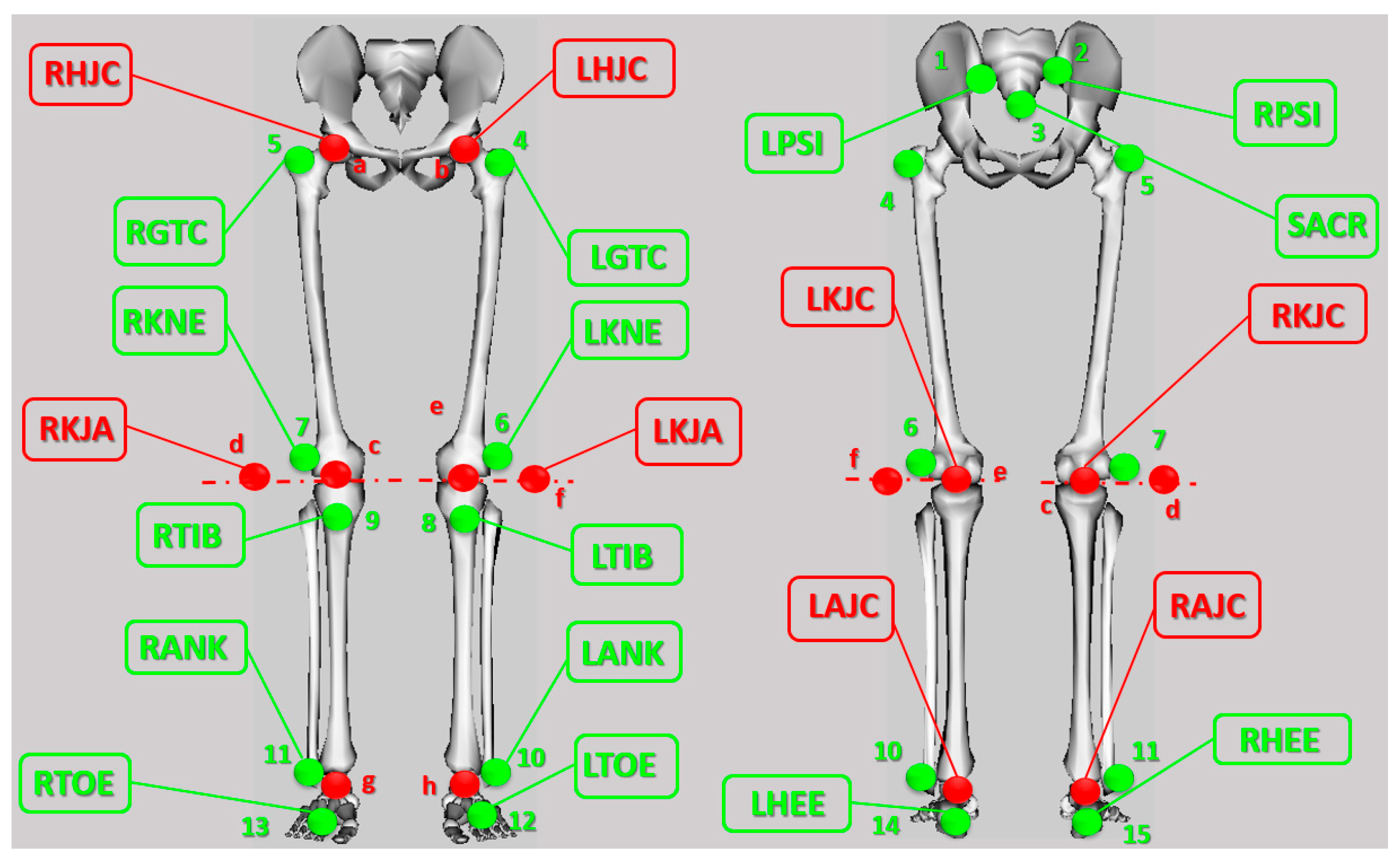
2.3. Marker Protocol

The present study was focused on the 3D kinematic analysis of the lower limb. The lower body was segmented as follows: one pelvis, two femurs, two tibias and two feet. A new marker protocol based on the PiG [24] protocol was developed for this study. The PP is a nonoptimal pose estimator based on a minimum number of markers placed on the subject. In total, 15 physical markers and 8 virtual markers were used (Figure 1). No interference was observed between the position of the markers of the PP and the bicycle in both the sagittal and frontal planes (Figure 2a,b). No kinematic constraints were imposed. The choice of physical marker locations was made with particular care to ensure that the markers were not hidden during pedalling. In addition, they were placed in areas with little movement of the soft masses.

The pelvis kinematics were modelled by placing two markers on the posterosuperior iliac spines (RPSI and LPSI) and one marker on the sacrum (SACR). The sacrum is a fairly large bone; so, to ensure that, for all participants, the location was equivalent, this marker was placed just above the intergluteal line. This disposition allowed us to eliminate the markers placed on the anterior iliac crests that, in the pedalling posture, were partially hidden and very influenced by the STA.

Figure 1 and Figure 2 show that in the thighs and legs, the markers placed in the fatty zones [24] were replaced by markers placed in the greater trochanter and in the tibial tuberosity, respectively. This change significantly reduces the sensitivity of the results to incorrect placement of the markers [24]. The marker arrangement in these solids is as follows: Thighs presented one marker placed on the greater trochanter (RGTC and LGTC) and another on the lateral epicondyle (RKNE and LKNE). The legs featured one marker placed on the tibial tuberosity (RTIB and LTIB) and another on the lateral malleolus (RANK and LANK).

Following the arrangement proposed by Davis et al. [24], two markers were placed on the foot: one on the calcaneus (RHEE and LHEE) and one on the second phalanx of the first metatarsal (RTOE and LTOE). When the participants are wearing shoes, it can be difficult to locate the two anatomical points where the markers should be placed. However, a procedure was developed that only requires the detection of one of the anatomical points. Firstly, a static capture was taken of the participant’s bare foot with the foot markers placed on the specified landmarks. Once the capture was made, the relative position between the foot markers was obtained. Depending on the participant, the HEE marker was sometimes easier to detect by feeling inside the shoe, while on other occasions, the TOE marker was easier. Using the computed relative position of the known marker, the location of the other foot marker could be obtained.

As previously mentioned, the protocol incorporates eight virtual markers. These markers are not physically placed on the participant during motion capture, which enhances participant comfort. They are added during the post-processing phase to define joint centres and axes of rotation. In the present study, virtual markers were employed to define the hip and ankle joint centres, as well as the knee axis of rotation. The hip centre (RHJC and LHJC) was calculated by the functional method SCoRE [29]. The knee rotation axis, which consisted of the knee joint centre (RKJC and LKJC) and an arbitrary point of the knee rotation axis (RKJA and LKJA), was determined from the functional methods SARA [30]. The ankle joint centre (RAJC and LAJC) was determined from the methodology developed by Davis et al. [24]. A table explaining in detail the position of each marker in the PP was included in the Supplementary Materials.

Static calibration was performed with the participant in standing anatomical position. The objective of these captures was to fit the model to the subject morphology. For this purpose, the deviations from the anatomical position were quantified with the idea of correcting them when performing body pose reconstruction, as carried out in PiG [24].

2.4. Body Pose Reconstruction Method

The position and orientation of each solid was reconstructed from the trajectories of the markers obtained experimentally. The orientation of the solids was defined using the recommendations of the ISB [31].

The joint angles were defined as the relative orientation of a solid with respect to its adjacent one. To obtain them, the procedure described in the study by Ojeda et al. [32] was used. This procedure was based on the use of rotation matrices for the calculation of the joint angles. The rotation matrices were obtained by determining the local reference systems of each solid, which are explained below. The reconstruction procedure was implemented in a custom-made calculation routine using Matlab R2024a (The MathWorks, Inc., Natick, MA, USA).

Because no kinematic constraints were imposed, it was necessary to use at least three non-collinear markers to reconstruct the local system of each solid.

The pelvis’ Lateral–Medial (LM) axis was determined from the direction between the RPSI and LPSI markers. The Antero–Posterior (AP) axis was defined as the normal to the plane formed by the RPSI, LPSI and SACR markers. The Cranio–Caudal (CC) axis was defined perpendicular to the AP and LM axes.

The thigh had only two physical markers; so, to obtain the local system for this solid, virtual markers were also used. In this case, the CC axis was calculated from the RHJC and RKJC markers. The AP axis was determined as the normal to the plane defined by the RGTC, RHJC and RKNE markers. The LM axis was defined perpendicular to the CC and AP axes.

The local leg system had to be defined using virtual markers in addition to the physical markers. The CC axis was formed from the RKJC and RAJC markers. The AP axis was defined from the normal to the plane formed by the RKJC, RKJA and RANK markers. The condition of perpendicularity to the CC and AP axes was established to determine the LM axis.

Virtual markers were also used, in this case, following the methodology established by Davis et al. [24]. The AP axis for this solid was calculated from the position of the RHEE and RTOE markers. The LM axis was obtained from the normal to the plane formed by the RHEE, RTOE and RAJC markers. The CC axis was defined perpendicular to the LM and AP axes.

The procedures above have been explained with the markers of the right leg. For the left leg, the procedure was equivalent.

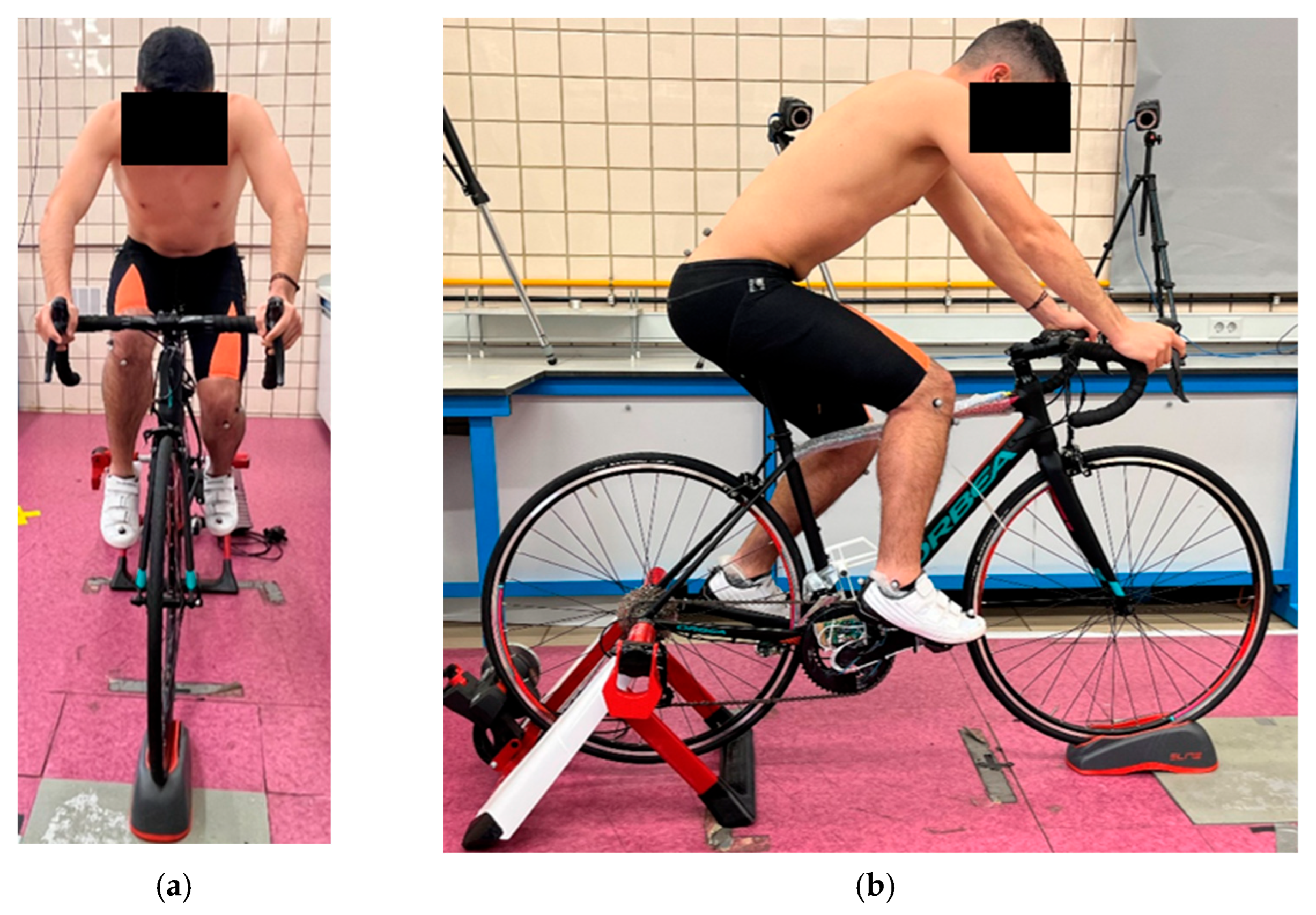
2.5. Test Conditions

Kinematic captures were carried out while maintaining a pedalling power of 170 W and 90 rpm of cadence, similar values to those used by other works [5,9,10].

In addition to this information, a pulse oximeter and individual measurement of maximum frequency were also used together with a basic health questionnaire in which personal history of injury was asked. Cardiopulmonary auscultation was performed, and oxygen saturation and resting heart rate were assessed. A medical research council (MRC) scale for assessment of dyspnoea with exercise was also performed. This scale was chosen because it is a sample of non-athletes.

Saddle height was established using the methodology developed by Holmes and Pruitt [33]. Right knee flexion was estimated using a goniometer (25–35°). To achieve greater comfort for each participant, the saddle height could be altered slightly, trying, in most cases, to ensure that the minimum angle of knee flexion was within the range established by Holmes and Pruitt [33]. The saddle used in this study was the same for all participants. It was a standard saddle purchased with the bicycle. It is 16 cm at its widest point and 5 cm at its narrowest point. The saddle has an anatomical hole. The use of the same saddle for all the participants is justified according to studies related to bicycle fit [22,34]. In these works, it is established that the design of the saddle is important, especially during prolonged use of the bicycle. This was not the case during the measurements performed in this work, where cycling did not exceed 10–15 min. In any case, the participants were checked for comfort by means of questions before, during and at the end of the study, and no results were obtained for discomfort due to the saddle.

Each test was divided into two parts. The first part, which involved the first 2–3 min of each test, was used as a warm-up and to verify that the subject felt comfortable pedalling with the selected saddle height and position on the bicycle. The second part started once the participant had acclimatised to the pedalling conditions. Only in this part were the recordings of the pedalling movement carried out. To prevent fatigue effects on the results obtained, only 5 trials of 10 s each were recorded for each participant. The time between captures was approximately 5–10 s.

2.6. Experimental Data Post-Processing

Experimental data were collected and processed with Vicon Nexus^® 2.12.1 commercial software. Based on residual analysis [35], the data were filtered with a low-pass filter (6 Hz, 4th order Butterworth filter) by a custom-made routine using Matlab R2024a (The MathWorks, Inc., Natick, MA, USA) to eliminate high-frequency noise [36,37].

2.7. Evaluation of the Proposed Protocol

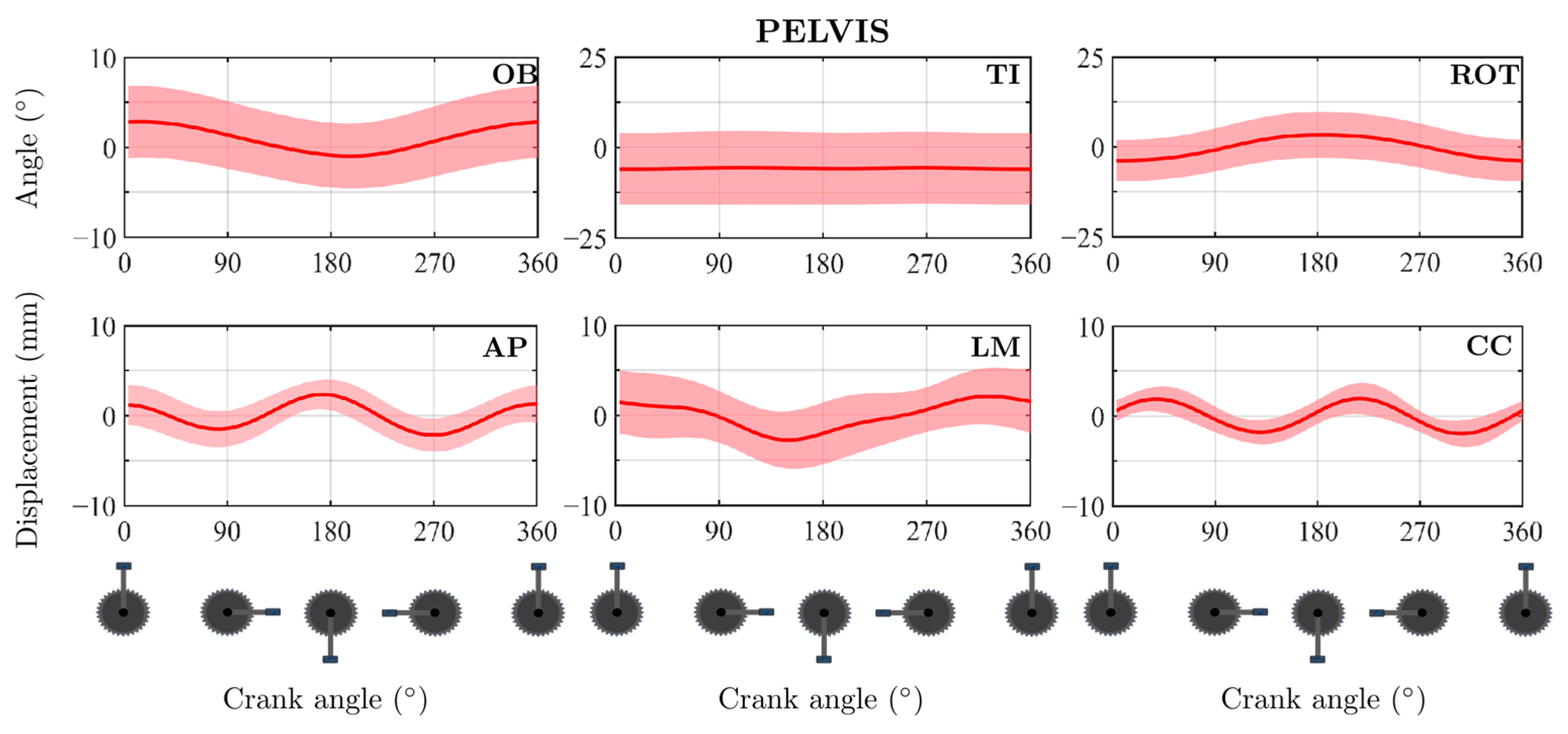
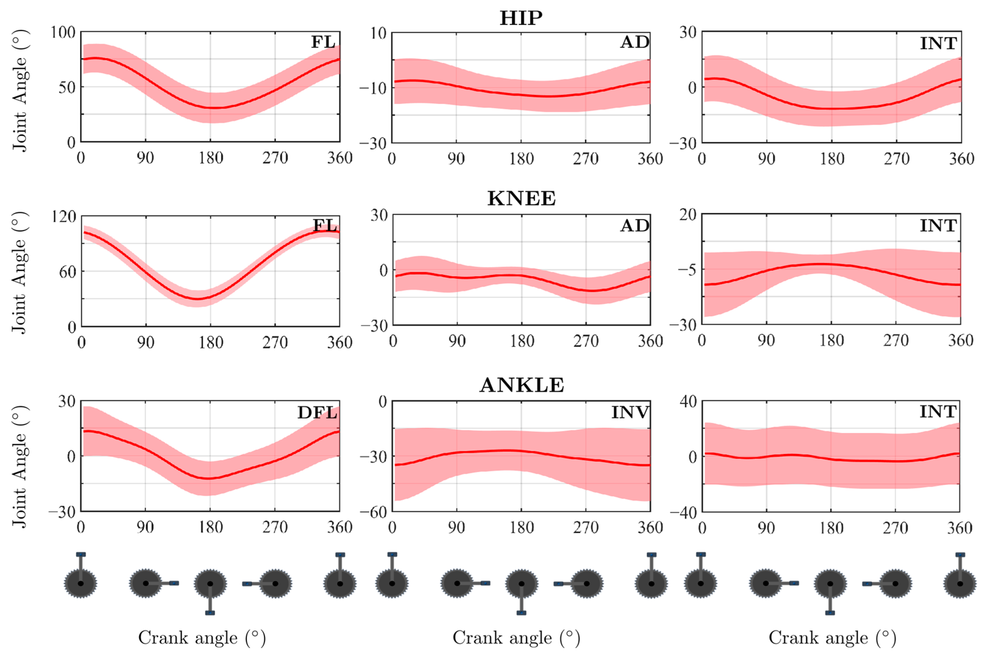
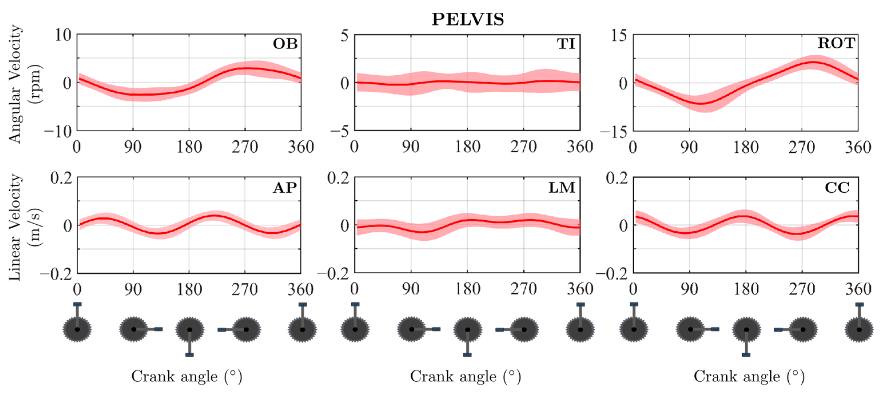
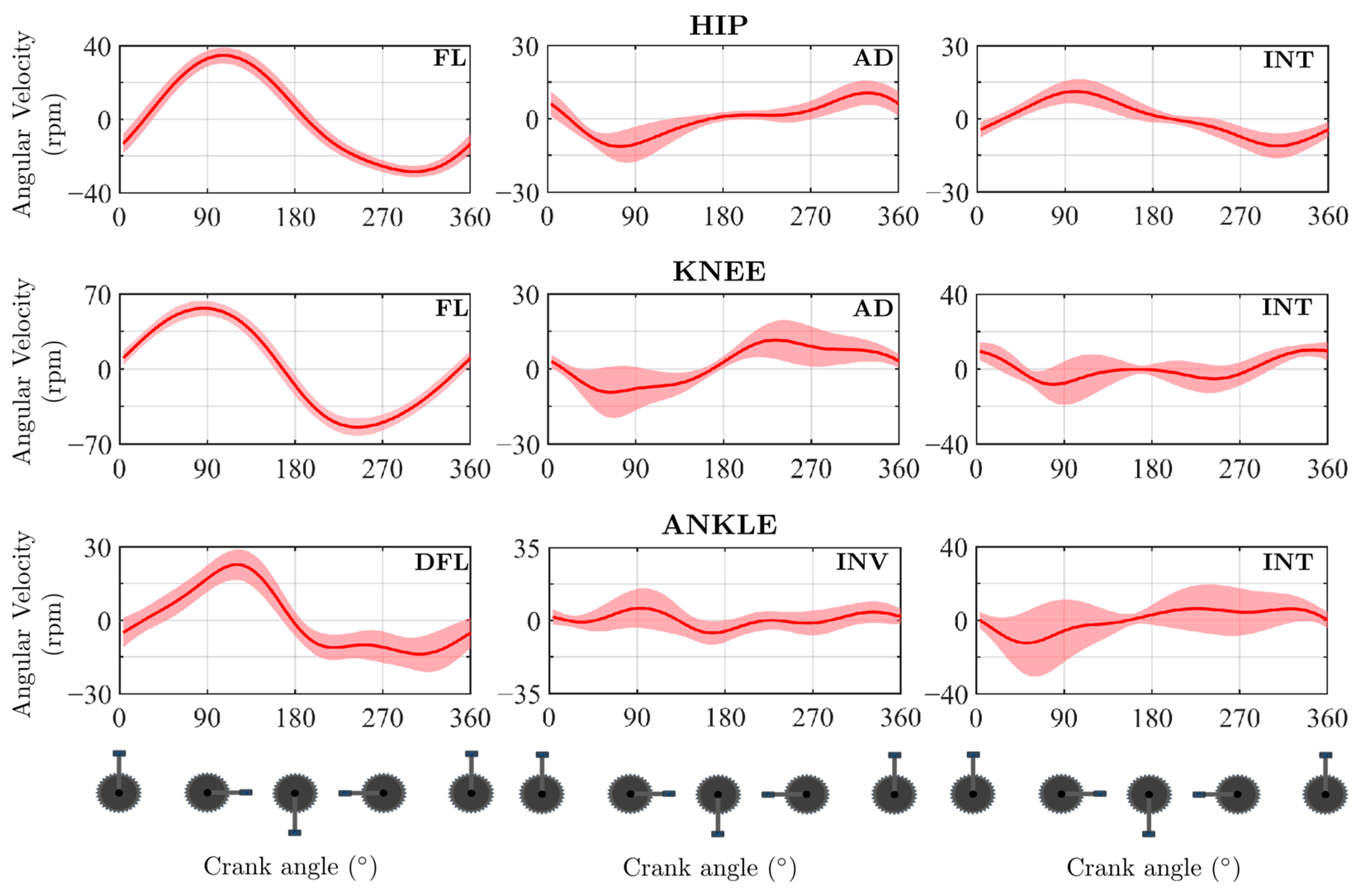
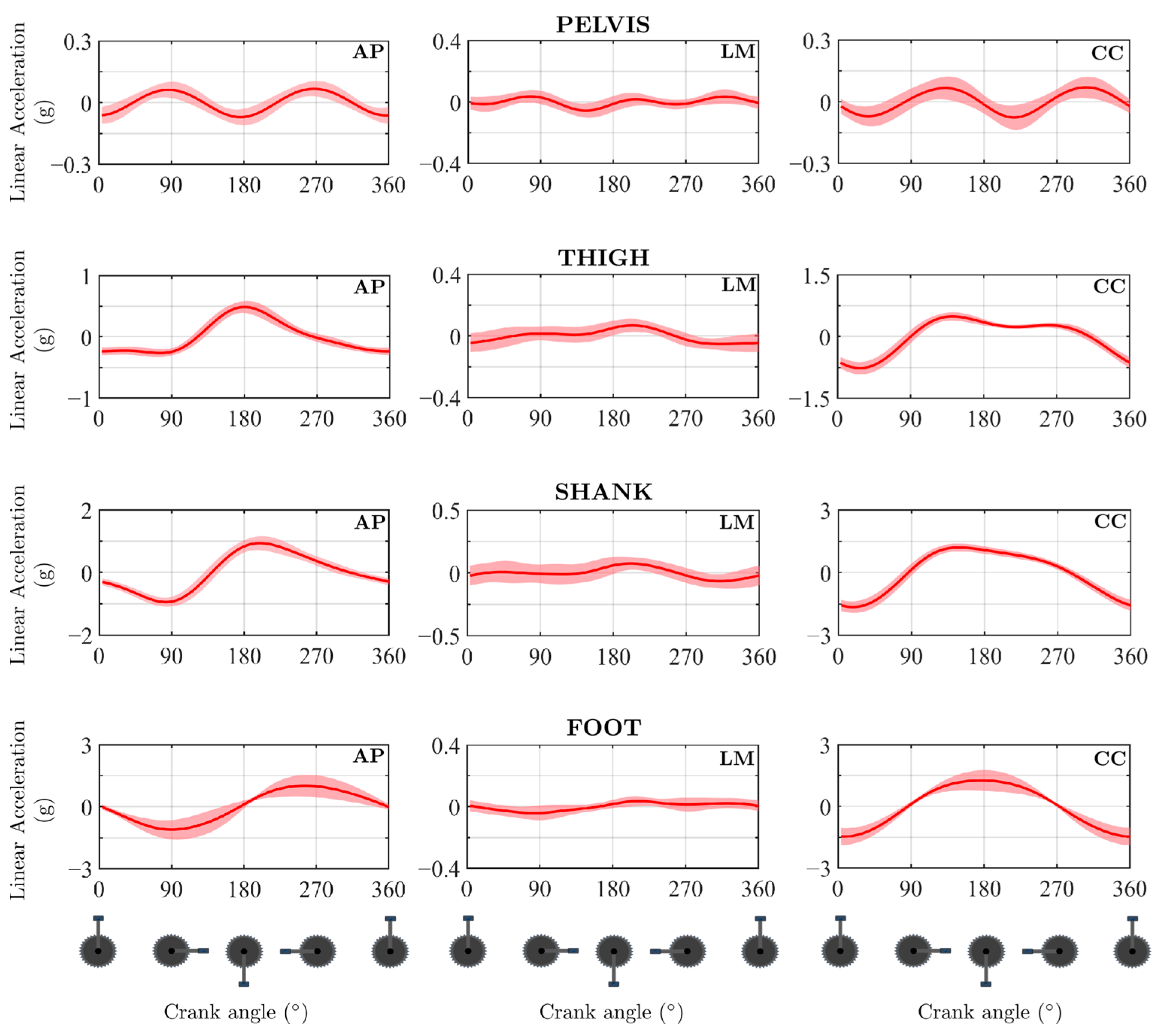
The evaluation of the PP was performed by comparing the kinematic results provided by this protocol in gait analysis with those obtained with two other protocols widely accepted by the scientific community: PiG [24] and the Cleveland modified protocol (CMP) [38]. Two study participants were fitted with sufficient markers to obtain kinematics with all three protocols and were asked to perform at least ten gait cycles. None of the participants had any gait pathology and walked at a freely chosen speed. The kinematics of each gait cycle were obtained with each of the reconstruction protocols. The CCC [39] was calculated for the three comparisons: PP vs. PiG, PP vs. CMP and PiG vs. CMP. The CCC is defined as follows:

$$CCC\left(k\right)={\displaystyle \frac{c_{{JA}_D{JA}_{ND}}\left(k\right)}{\sqrt{\sum _{t=1}^N{\left({JA}_{MP1}\left(t\right)-\overline{{JA}_{MP1}}\right)}^2\ast \sum _{t=1}^N{\left({JA}_{MP2}\left(t\right)-\overline{{JA}_{MP2}}\right)}^2}}}$$

(1)

where:

$$c_{{JA}_{MP1}{JA}_{MP2}}\left(k\right)=\left\{\begin{array}{c}{A}_{{JA}_{MP1}{JA}_{MP2}}\left(k\right)+B_{{JA}_{MP1}{JA}_{MP2}}\left(k\right),ifk\in \left[1,N\right]\\ \\ \hspace{1em}\hspace{1em}\hspace{1em}\hspace{1em}\hspace{1em}{A}_{{JA}_{MP1}{JA}_{MP2}}\left(k\right),ifk=0\end{array}\right.$$

(2)

where:

$$A_{{JA}_{MP1}{JA}_{MP2}}\left(k\right)=\sum _{t=1}^{N-k}\left({JA}_{MP1}\left(t\right)-\overline{{JA}_{MP1}}\right)\ast \left({JA}_{MP2}\left(t+k\right)-\overline{{JA}_{MP2}}\right)$$

(3)

$$B_{{JA}_{MP1}{JA}_{MP2}}\left(k\right)=\sum _{t=N-k+1}^N\left({JA}_{MP1}\left(t\right)-\overline{{JA}_{MP1}}\right)\ast \left({JA}_{MP2}\left(t-N+k\right)-\overline{{JA}_{MP2}}\right)$$

(4)

In Equation (1), CCC(k) represents the cross-correlation coefficient for a time shift k between the same joint angle obtained by different markers protocols. For the set of equations, ${JA}_{MP1}\left(t\right)$ and ${JA}_{MP2}\left(t\right)$ represent the same joint angles of the markers’ protocol 1 and the markers’ protocol 2 at each instant of time t. N is the number of instants that compose the gait cycle. $\overline{{JA}_{MP1}}$ and $\overline{{JA}_{MP2}}$ represent the average value of the joint angle performed by the markers’ protocol 1 and the markers’ protocol 2 over the analysed gait cycle, respectively. ${\tau }_{lag}$ is defined as the joint angle delay and indicates the lag of the markers’ protocol 2 joint angle with respect to the markers’ protocol 1 joint angle. It corresponds to the value of k at which the correlation coefficient CCC(k) is maximum. A ${\tau }_{lag}$ positive value indicates that the markers’ protocol 2 joint angle is shifted forward in the gait cycle relative to the markers’ protocol 1. The CCC(k) oscillates in the interval (−1–1), with the maximum value corresponding to the best overlap between the joint angles on both markers’ protocols evaluated.

3. Results

Table 1. Average values of the cross-correlation coefficient and ${\tau }_{lag}$ for a representative participant. The results are shown as the average ± standard deviation.

Joint	Joint Angle	PP vs. CMP		PP vs. PiG		PiG vs. CMP
		CCC	${\mathit{\tau }}_{\mathit{l}\mathit{a}\mathit{g}}$(%)	CCC	${\mathit{\tau }}_{\mathit{l}\mathit{a}\mathit{g}}$(%)	CCC	${\mathit{\tau }}_{\mathit{l}\mathit{a}\mathit{g}}$(%)
Hip	FL	0.979 ± 0.006	2.4 ± 0.5	0.991 ± 0.004	0.6 ± 0.5	0.991 ± 0.001	1.4 ± 0.5
	AD	0.805 ± 0.014	−1.4 ± 0.5	0.914 ± 0.014	0 ± 0	0.950 ± 0.010	0 ± 0.0
	INT	0.437 ± 0.120	−28.6 ± 17.3	0.533 ± 0.084	−19.6 ± 18.5	0.828 ± 0.022	−0.2 ± 0.4
Knee	FL	0.996 ± 0.001	−1 ± 0.0	0.998 ± 0.000	0 ± 0	0.994 ± 0.001	−1 ± 0.0
	AD	0.898 ± 0.016	−2.6 ± 0.5	0.760 ± 0.063	−4 ± 0.7	0.837 ± 0.023	0.2 ± 0.4
	INT	0.741 ± 0.035	13.2 ± 0.4	0.745 ± 0.014	4.8 ± 0.4	0.660 ± 0.032	6.4 ± 0.5
Ankle	DFL	0.883 ± 0.006	−2 ± 0.0	0.991 ± 0.001	0 ± 0	0.840 ± 0.013	−2 ± 0.0
	INV	0.750 ± 0.043	−39.6 ± 1.8	0.942 ± 0.015	−6.2 ± 0.4	0.779 ± 0.043	−33 ± 1.4
	INT	0.583 ± 0.095	9.2 ± 2.3	0.967 ± 0.010	−0.2 ± 0.4	0.588 ± 0.094	9.6 ± 2.3

Abbreviations: FL = Flexion (Sagittal plane). AD = Adduction (Frontal plane). INT = Internal Rotation (Transverse plane). DFL = Dorsiflexion (Sagittal plane). INV = Inversion (Frontal plane).

shows the average value of the CCC and ${\tau }_{lag}$ obtained by comparing the PP with the CMP in one of the two participants analysed. This table also includes the comparison between the PP and PiG. Finally, this table also shows the value of the CCC and ${\tau }_{lag}$ calculated by comparing the PiG and the CMP.

Figure 3 and Figure 4 reflect the average temporal evolution (TE) of all pedalling cycles analysed for the 19 participants of the pelvis 3D angles and movement and the 3D joint angle of the hip, knee and ankle. The pelvis movements were referenced against its centre of mass (CoM) obtained from the correlations developed by De Leva [40].

Figure 5 shows the intra- and inter-subject coefficient of variation (CV) [41] of the ROM for the pelvic CoM displacements and rotations and the hip, knee and ankle joint angles during pedalling. To obtain the inter-subject CV, all ranges of each movement analysed for the 19 participants were analysed globally. The intra-subject CV for each ROM was obtained as the average value of the CV of the 19 participants analysed.

Figure 6 reflects the average TE of all the pedal cycles analysed for the 19 participants of the CoM pelvis 3D angular and linear velocity. Similarly, Figure 7 shows the TE of the 3D joint velocity of hip, knee and ankle joint. The same pedal cycles analysed previously were analysed for this case. Joint velocity was obtained following the procedure described in the paper by J. Ojeda et al. [32].

Finally, Figure 8 shows, in global coordinates, the average of the TE of the linear accelerations of the pelvis, thigh, leg and foot CoM. As in the case of the pelvis, the CoMs for the rest of the solids that compose the lower body were calculated using the methodology developed by De Leva [40].

4. Discussion

4.1. Proposed Protocol Evaluation

Table 1 shows that high CCC values are obtained when comparing the PP with the PiG and with the CMP in the joint variables contained in the sagittal plane. These results highlight the interest of this work since it suggests that, in cycling, similar results to those provided by protocols accepted by the scientific community can be obtained in the sagittal plane, but with a more stable and comfortable placement of markers for the participant and a simpler procedure.

Outside the sagittal plane, the PP shows a high correlation with the PiG in the hip and ankle with CCC values above 90% for all joint variables. The exception was hip internal rotation where it shows a medium correlation value (53%) and a gait cycle lag of 20%. These results are slightly worse when correlating the PP with PCM for hip variables and worse for ankle variables. However, this difference in results is also apparent when analysing the CCC between the PiG and the CMP. The reduced CCC values observed for hip internal rotation may be attributed to several factors. One such factor, previously discussed in this paper, is the fundamental difference between the protocols: the PP employs a non-optimal pose estimation approach, whereas the CMP utilises a Least-Squares Pose Estimation method. As a result, the PP is highly sensitive to marker placement, and even minor discrepancies in marker positioning can lead to noticeable variations in the calculated kinematics. Conversely, the CMP is more robust to such misplacements due to its reliance on a greater number of markers. However, this increase in marker count may compromise participant comfort during testing. Another consideration, particularly relevant when comparing internal rotation values between the PP and PiG, is the inherently low ROM of this movement, typically around 10°. Such a limited ROM increases the relative impact of minor marker misalignments, potentially affecting both the magnitude and sequence of the observed motion. This underscores the importance of meticulous marker placement when using non-optimal estimation protocols. To mitigate variability introduced by inconsistent marker placement, it is recommended that the same operator apply the markers across all participants. In this work, this methodology was adhered to throughout the experimental protocol. On the other hand, the ankle–foot complex is, along with the shoulder complex, one of the most difficult to analyse accurately in the human body. The results provided by different protocols for the same movement provide a wide dispersion, as shown by Ferrari et al. [42]. However, this limitation is less pronounced in the present study since the pedalling analysis used shoes with cleats, which considerably reduced the possible movements of the foot–ankle outside the sagittal plane.

Regarding knee joint variables outside the sagittal plane, it is observed that the PP correlates better with CMP in the frontal plane than with the PiG. This was to be expected since one of the limitations of the PiG is the estimation of knee joint variables outside the frontal plane if devices such as the Knee Alignment Device [43] (KAD) are not used. The KAD is a device which is composed of three reflective markers that form a directional trihedron which is placed on the knee of the participant to be tested. The objective of using the KAD is to assist the PiG in the automatic definition of the direction of the knee flexion axis during a static trial. The correlations of internal rotation of the knee present average values in all three comparisons. Again, this is to be expected due to the reduced ROM in the transverse plane [42].

4.2. Position Problem

The results of the position problem were analysed from two different approaches. First, they were analysed from a physiological point of view by checking the physical meaning of the results and comparing them with results published in the literature obtained under similar test conditions. Second, a discussion of the intra-subject and inter-subject variability in the results obtained was carried out to determine the robustness of the PP.

The pelvis’ movements as a rigid solid (Figure 3) show small rotations in the sagittal and frontal planes and larger rotations in the transverse plane, a behaviour in accordance with that shown by other authors in their works [8,15]. Similarly, the displacements of the CoM of the pelvis show an oscillatory behaviour around the resting position on the saddle. In particular, the displacements in the AP and CC directions show an oscillation frequency twice that of the displacement in the LM direction. Thus, the pelvis moves to the left during the first phase of the cycle and to the right in the second phase. The pelvis CoM performs a complete cycle of displacement in the AP and CC direction in each half of the cycle because of the extension and flexion mechanism performed in each phase of the pedalling cycle. In general, the movements performed by the pelvis are mainly due to compensatory mechanisms of the body to perform the technical gesture of pedalling. These mechanisms generally tend to be magnified in amateur cyclists and even in professional cyclists because of fatigue [6].

The knee’s flexion–extension movement (Figure 4) presents the greatest ROM during the entire pedalling cycle, approximately 75°. This value is similar to that found in the literature [5,11,15,17]. The TE of this movement shows how an extension of the knee occurs from the beginning of the pedalling cycle (0°) to approximately 160°, in what is known as the power phase [28]. The maximum knee extension occurs just before bottom dead centre (BDC), in concordance with some papers in the literature [5,9,10]. Once the power phase is overcome, the pedal recovery phase begins (180–360°). In this phase, maximum knee flexion occurs when the crank angle is approximately 345°, a value in agreement with the literature [5,9,10,15].

Knee movement in the frontal plane shows an ROM close to 10°, in line with that shown by other works [5,11,12,13]. This movement TE shows that positive values are hardly achieved; so, participants tend to spend the whole pedalling cycle in knee abduction. The abduction presents two maximums: the first with a value of 5° when the crank is positioned at 90°, and the second approximately 13° when the crank is close to 270°. This behaviour coincides with that shown by other authors in their work [3,9,15,16]. Between both maximums, abduction presents a valley with a value close to 0° at the instant when the crank forms 170° with the vertical, coinciding with the moment of least knee flexion. This fact is due to the internal and external collateral ligaments, which are responsible for stability in the lateral–medial direction of the knee, decreasing the capacity of movement in the frontal plane when the knee is more extended due to the tension of them. In addition to these ligaments, the sartorius, semitendinosus, rectus femoris and tensor fasciae latae muscles act as active ligaments contributing to this lateral–medial stability. The tensor fasciae latae causes an external rotation of the knee when it is extended, as can be seen in Figure 4, where there is a smooth decrease in internal rotation that disappears when knee flexion is initiated again. The instants in the pedalling cycle when the maximum internal rotation of the knee occurs coincide with the moments when the highest values of hip adduction are observed—specifically, when the knee is nearest the midline of the body. This is mainly due to the action of the adductor and gracilis (rectus internus) muscles. This behaviour in the internal rotation of the knee, together with its ROM, approximately 5°, is close to that obtained by other authors in their studies [3,9,15,16].

The sagittal plane hip movement (Figure 4) shows a similar behaviour to knee flexion. An extension of this joint is observed from the beginning of the cycle to 150–160°, similarly to that shown by other authors [5,9,10]. Moving to the pedal recovery phase, hip flexion occurs again, coinciding with knee flexion. In this plane, the hip shows an ROM close to 40–45°, in line with that shown by other works [3,9,10,15,16]. The maximum hip flexion value agrees with that shown by Ferrer-Roca et al. [44] and Ericson et al. [2] in their work. Due to the existence of bi-articular muscles that act on both joints (hip and knee), the maximum and minimum reached in knee flexion can affect those of the hip, being the determination of the saddle height a fundamental parameter when optimising these values.

The frontal plane hip movement shows an ROM around 8°, close to that reported by Pouliquen et al. [11] and Galindo-Martinez et al. [15]. The negative value indicates a hip abduction, behaviour in accordance with that reported by some authors [5,9,10,15]. The instant of maximum adduction, reached when the crank is close to the top dead centre (TDC), coincides with the instant of maximum hip flexion, registering values close to −10°, of the order as shown by other authors [5,9,15]. The minimum adduction is reached shortly after passing through the BDC, similar to that shown by Galindo-Martínez et al. [15] in their work.

Concerning the hip movement in the transverse plane, it shows an ROM close to 15°, in line with what is reported in some of the studies [5,9,10,11]. In most of the pedalling cycle, an external rotation of the hip is observed. This movement TE is strongly influenced by the flexion and rotation of the knee. Knee rotation values are maximum near the TDC while hip external rotation values are minimum. When the knee is extended, near the BDC, the rotation capacity of this joint is practically null, as shown in Figure 4. This causes the rotation capacity of the lower body to fall entirely on the hip, which reaches the maximum value of external rotation at this point. A similar behaviour to the one explained above is found in other studies [5,9].

The dorsiflexion–plantarflexion (DFL-PFL) of the ankle presents an ROM in the order of 25°, in agreement with that shown by other authors [11,17]. This movement TE shows both DFL and PFL. These curves’ pattern shows that the DFL movement reaches its maximum value at the beginning of the cycle, because the rearfoot movement is the ideal one for the pedal push. Subsequently, the value of this movement decreases until it reaches 0º near the instant when the crank is forming 90° with the vertical, at which time the effective force applied to the pedals is at its maximum. This behaviour is in accordance with that shown by Bini and Carpes [28]. From this instant, the ankle is in PFL, and the value of this movement increases until it reaches its maximum when the pedal is close to the BDC, because it is at this point that the leg is more stretched. From this point onwards, the PFL ankle movement decreases and tends to a DFL movement near the end of the cycle. This is because, as the crank approaches 345°, the anterior leg muscles at the ankle level and the ilio-psoas, tensor fasciae latae and sartorius at the knee and hip level extend the leg positioning the foot for the beginning of the next power phase [28].

The movements of the ankle outside the sagittal plane are those that show the greatest dispersion of results in the literature as well as in this work. The ROM of ankle inversion and internal rotation movements shown in Figure 4 are of the order of 7° and 4°, respectively, in accordance with those shown by other authors [9,10,11,12,15,16]. However, as mentioned above, the dispersions at these joint angles are high. This fact may be due to several reasons; the first one is related to the pedalling technique and experience of the analysed participants. Another reason may be due to the shoes’ influence and pedal type, especially at the ankle rotation level. This joint angle is in function of the cleats used and the rotation freedom they allow, and this movement may have a greater or lesser ROM.

Intra-subject analysis from the CV of ROMs, as shown in Figure 5, showed a variability in the pelvis close to 15% in the sagittal and transverse plane rotations and of 30% in the frontal plane. The variability in pelvic displacements showed values higher than 15% in all three directions of space. In general, the variability present in the pelvis is explained by the reduced movements that occur in this biomechanical segment during pedalling.

The analysis of intra-subject variability in the joints showed very low values in the sagittal and transverse planes for the hip and knee. The greatest variations were found in the frontal plane of these joints, although they did not exceed 15% in any of the cases. This behaviour was due to the fact that, as shown in Figure 3 and Figure 4, this plane shows reduced ROMs; so, the results were more sensitive to small variations in the placement of the markers and in the movements performed.

The analysis of intra-variability in the case of the ankle showed similar variability in all three planes, somewhat higher than for the other two joints, although in no case did the CV value exceed 15%. This behaviour of the ankle may be due to the lack of practice the participants had in pedalling with cleats and clipless pedals. This discussion is reinforced by analysing the results shown in the Supplementary Materials appended to this paper.

In the analysis of inter-variability based on the CV of the ROMs, higher values than those obtained with the analysis of intra-variability were obtained, which is reflected in the literature [40]. In this study, the variability is quite small in the hip and knee. Outside the sagittal plane, the variability is much higher. Again, the results at the ankle show high variability in all three planes. There are several reasons for these results. From a biomechanical point of view, the mechanism formed by the thigh, leg and foot with the pedal, crank and bicycle frame has different mounting branches. Thus, the same crank position can be achieved with different leg positions. This phenomenon may occur especially in non-professional cyclists without a mature pedalling technique.

However, no data have been found in the literature to confirm this hypothesis. A study with professional cyclists in this sense would therefore be of interest. Another aspect to consider is the morphology of the participants. The saddle height was adjusted for each participant. However, this did not imply that the resulting equivalent mechanisms were similar. The reason is that the ratio between segment lengths in the biomechanical model does not generally hold.

4.3. Velocity Problem

The results obtained showed similarities with those shown in the literature, especially in the sagittal plane, where they present values of the order of those obtained by Sinclair et al. [9]. The ankle in the sagittal plane also presents a value and TE similar to those obtained in the literature [9]. Outside the sagittal plane, there are also high similarities, as in the case of hip and knee internal rotation. In the frontal plane, the hip has an ROM similar of that obtained by Sinclair et al. [9].

Figure 7 also shows that the maximum hip abduction and internal rotation velocities are in the order of 20–30% of the maximum hip flexion velocity at this joint. In the case of the knee, 10–20%, and in the case of the ankle, the maximum inversion and internal rotation velocities are generally 35–45% lower than the absolute maximum PFL velocities.

These results highlight the interest of analysing angular velocities outside the sagittal plane and that significant values of movements outside the sagittal plane could play an important role in the estimation of joint-specific powers, as stated by the authors in a previous work [26].

4.4. Acceleration Problem

A segmental analysis in Figure 8 shows that the acceleration values decrease as one moves up from the foot to the thigh, which is explained by analysing the equivalent mechanism. The foot performs a rotational movement which generates a centrifugal acceleration that is directly dependent on the angular velocity squared and the radius of rotation, which is approximately equal to the crank length. The pedalling speed was defined as constant. It was experimentally proven that this is true on average, although participants produce slight oscillations in angular velocity during the pedalling cycle [26]. Therefore, the tangential acceleration is approximately zero. In the case of the thigh, it is performing an alternating rotational movement with an angular velocity of the order of one third of the pedalling cadence and a rotation radius that is of the order or higher than the length of the crank. This result implies that both tangential and centrifugal accelerations are lower than those of the foot.

A component analysis shows that the largest accelerations occur in the sagittal plane (except for the pelvis), with the CC component being slightly greater than the AP. This is explained by the fact that in the CC direction, the inertial forces have to balance the gravity action. Usually, kinematics outside the sagittal plane are not considered in cycling practice because they present an ROM orders of magnitude lower than that in the sagittal plane, being these assumptions generally extended to the dynamic analysis. However, in the results obtained in this work (Figure 8), it can be observed that the acceleration in the LM direction of the thigh can reach a value between 20% and 30% of the acceleration in the sagittal plane. Therefore, the authors of this paper argue that the values obtained in the LM direction, although small compared to the other two components, should not be underestimated. The accelerations obtained imply the appearance of inertia forces, which cannot be negligible in the overall balance of the system, especially in the estimation of the stresses to which the joints are subjected. Joint reaction force calculations are key to assessing performance and possible injury in cyclists. No results have been found in the literature that develop this hypothesis. Preliminary results obtained by the authors indicate that accelerations can cause forces of inertia in the LM direction of the same order of magnitude of the total resultant force in this direction that the joint is subjected to, especially in positions around the TDC or the BDC.

4.5. Examples of Protocol Applicability

In the last two decades, studies have shown that, in addition to movement in the sagittal plane, there are important movements in the frontal and transverse planes [9,45,46]. Recently, 3D motion analysis has become a crucial tool in addressing rehabilitation processes related to cycling [16].

Patellofemoral syndrome (“cyclist’s knee”) is the most common cause of knee pain in the cyclist [21]. This pain is caused by increased pressure in the patellofemoral joint. Factors like low or anterior saddle position, or excessively long cranks, lead to higher values of the knee flexion angle at the top of the pedal stroke, producing an increase in the patellofemoral contact pressure [22].

Maltracking knee is often accompanied by a decrease in gluteus-medius-generated force, the appearance of contralateral pelvic tilt, valgus knee deviation, and foot pronation [47]. Detection of this behaviour is essential to reduce or eliminate knee joint pain. The most common treatment is to increase recruitment of the gluteus medius and vastus medialis obliquus. In addition, it is necessary to improve the alignment of the foot and ankle on the bicycle to improve the mechanics of the knee and, consequently, reduce pain. The implementation of the proposed protocol can be of great use in clinical practice by allowing for the quantification of kinematic deviations in the pelvis, knee and foot, some of which, as mentioned above, occur outside the sagittal plane.

4.6. Limitations

In this section, the limitations of this study are described. One of these limitations is the fact that only two participants were used for the comparison of the PP with other marker protocols during the gait cycle analysis. This meant that a statistical analysis could not be performed because the statistical power would be too low.

Another limitation of this work is the fact that only men were analysed. This is because the aim was to assess the PP; so, a homogeneous sample of participants was sought. As some studies [48,49] indicate, when pedalling, the saddle affects men and women differently, and this may end up affecting the final results. As a future study linked to this idea, we could analyse whether there are statistically significant differences in the 3D kinematics of pedalling between men and women.

Finally, this study analysed participants with a non-professional character in cycling. This fact may affect the discussion of the results, especially when comparing them with studies that show the kinematics during pedalling but for professional cyclists. As a future study, a comparison of the 3D pedalling kinematics between professional and amateur cyclists could be considered.

4.7. Advantages of This Study

The main advantage of this study is that the PP offers remarkable practical applicability in pedalling tasks where conventional protocols encounter significant limitations, as was discussed. Another significant advantage of the PP is that it does not require the definition of a technical axis system and a subsequent transformation to an anatomical system and is therefore more efficient. Finally, the virtual markers for the hip centres and the knee flexion axis were defined using functional methods to make the protocol as close as possible to the participant.

5. Conclusions

A new protocol has been developed to measure 3D pedal kinematics based on a non-optimal procedure. The number of physical markers used has been reduced to avoid loss of markers due to masking or artefacts due to soft mass movements.

Protocol evaluation through its application to gait analysis has found that it correlates very well with other widely accepted protocols in the literature, especially in the sagittal plane. Those joint angles that have shown a lower correlation are defined outside the sagittal plane and are more difficult to quantify accurately with this technology, regardless of the marker protocol used. In any case, the conclusions obtained in the gait analysis can be extrapolated to cycling since the markers of the new protocol are in positions where there is no presence of large soft masses. Therefore, in response to the first research question, the proposed protocol provides kinematic results in pedalling analysis that are equivalent in accuracy and repeatability to protocols commonly used in gait analysis.

In answer to the second question posed in the motivation of this paper, joint angles outside the sagittal plane may account for 30–40% of the maximum values reached in the sagittal plane, especially in the ankle. The results obtained have shown that angular velocities occurring outside the sagittal plane are not negligible, reaching values up to 35–45% of the velocities contained in the sagittal plane. Therefore, when estimating joint powers, it is advisable to consider the components in the frontal and transverse planes. Similarly, linear accelerations outside the sagittal plane are smaller than those contained in the sagittal plane reaching maximum values in the order of 20–30% of the maximum value contained in the sagittal plane. The preliminary results obtained by the authors of this paper suggest that inertial effects outside the sagittal plane should not be neglected and can be very important, especially at positions such as the TDC and BDC. These conclusions will be developed in a future paper.

References

1. Fonda, B.; Sarabon, N.; Li, F. Validity and reliability of different kinematics methods used for bike fitting. J. Sports Sci. 2014, 32, 940–946. [Google Scholar] [CrossRef]
2. Ericsson, M.O.; Nissel, R.; Németh, G. Joint Motions of the Lower Limb during Ergometer Cycling. J. Orthop. Sports Phys. Ther. 1988, 9, 273–278. [Google Scholar] [CrossRef]
3. Umberger, B.R.; Martin, P.E. Testing the Planar Assumption During Ergometer Cycling. J. Appl. Biomech. 2001, 17, 55–62. [Google Scholar] [CrossRef]
4. Vrints, J.; Koninckx, E.; Van Leemputte, M.; Jonkers, I. The Effect of Saddle Position on Maximal Power Output and Moment Generating Capacity of Lower Limb Muscles During Isokinetic Cycling. J. Appl. Biomech. 2011, 27, 1–7. [Google Scholar] [CrossRef] [PubMed]
5. Cordillet, S.; Bideau, N.; Bideau, B.; Nicolas, G. Estimation of 3D Knee Joint Angles during Cycling Using Inertial Sensors: Accuracy of a Novel Sensor-to-Segment Calibration Procedure Based on Pedaling Motion. Sensors 2019, 19, 2474. [Google Scholar] [CrossRef]
6. Bini, R.R.; Diefenthaeler, F. Kinetics and kinematics analysis of incremental cycling to exhaustion. Sports Biomech. 2010, 9, 223–235. [Google Scholar] [CrossRef] [PubMed]
7. Bini, R.R.; Tamborindeguy, A.C.; Mota, C.B. Effects of Saddle Height, Pedaling Cadence, and Workload on Joint Kinetics and Kinematics During Cycling. J. Sport Rehabil. 2010, 19, 301–314. [Google Scholar] [CrossRef]
8. Bini, R.R.; Dagnese, F.; Rocha, E.; Silveira, M.C.; Carpes, F.P.; Mota, C.B. Three-dimensional kinematics of competitive and recreational cyclists across different workload during cycling. Eur. J. Sport Sci. 2016, 16, 553–559. [Google Scholar] [CrossRef]
9. Sinclair, J.; Hebron, J.; Atkins, S.; Hurst, H.; Taylor, P.J. The influence of 3D kinematic and electromyographical parameters on cycling economy. Acta Bioeng. Biomech. 2014, 16, 89–95. [Google Scholar]
10. Sinclair, J.; Hebron, J.; Hurst, H.; Taylor, P.J. The influence of different cardan sequences on three-dimensional cycling kinematics. Hum. Mov. Sci. 2013, 14, 334–339. [Google Scholar] [CrossRef]
11. Pouliquen, C.; Nicolas, G.; Bideau, B.; Garo, G.; Megret, A.; Delamarche, P.; Bideau, N. Spatiotemporal analysis of 3D kinematic asymmetry in professional cycling during an incremental test to exhaustion. J. Sports Sci. 2018, 36, 2155–2163. [Google Scholar] [CrossRef] [PubMed]
12. Hébert-Losier, K.; Yin, N.S.; Beaven, C.M.; Tee, C.C.L.; Richards, J. Physiological, kinematic, and electromyographic responses to kinesiologytype patella tape in elite cyclists. J. Electromyogr. Kinesiol. 2019, 44, 36–45. [Google Scholar] [CrossRef] [PubMed]
13. Thorsen, T.; Strohacker, K.; Weinhandl, J.T.; Zhang, S. Increased Q-Factor increases frontal-plane knee joint loading in stationary cycling. J. Sport Health Sci. 2020, 9, 258–264. [Google Scholar] [CrossRef] [PubMed]
14. Millour, G.; Duc, S.; Puel, F.; Bertucci, W. Physiological, Biomechanical and subjective effects of medio-lateral distance between the feet during pedaling for cyclists of different morphologies. J. Sports Sci. 2021, 39, 768–776. [Google Scholar] [CrossRef]
15. Galindo-Martínez, A.; López-Valenciano, A.; Albaladejo-García, C.; Vallés-González, J.M.; Elvira, J.L.L. Changes in the Trunk and Lower Extremity Kinematics Due to Fatigue Can Predispose to Chronic Injuries in Cycling. Int. J. Environ. Res. Public Health 2021, 18, 3719. [Google Scholar] [CrossRef]
16. Yum, H.; Kim, H.; Lee, T.; Park, M.S.; Lee, S.Y. Cycling kinematics in healthy adults for musculoskeletal rehabilitation guidance. BMC Musculoskelet. Disord. 2021, 22, 1044. [Google Scholar] [CrossRef]
17. Pouliquen, C.; Nicolas, G.; Bideau, B.; Bideau, N. Impact of Power Output on Muscle Activation and 3D Kinematics During an Incremental Test to Exhaustion in Professional Cyclists. Front. Sport Act. Living 2021, 2, 516911. [Google Scholar] [CrossRef]
18. Ojeda, J.; Martínez-Reina, J.; Mayo, J. A method to evaluate human skeletal models using marker residuals and global optimization. Mech. Mach. Theory 2014, 73, 259–272. [Google Scholar] [CrossRef]
19. McLeod, W.D.; Blackburn, T.A. Biomechanics of knee rehabilitation with cycling. Am. J. Sports Med. 1980, 8, 175–180. [Google Scholar] [CrossRef]
20. Farrell, K.C.; Reisinger, K.D.; Tillman, M.D. Force and repetition in cycling: Possible implications for iliotibial band friction syndrome. Knee 2003, 10, 103–109. [Google Scholar] [CrossRef]
21. Wanich, T.; Hodgkins, C.; Columbier, J.A.; Muraski, E.; Kennedy, J.G. Cycling injuries of the lower extremity. J. Am. Acad. Orthop. Surg. 2007, 15, 748–756. [Google Scholar] [CrossRef] [PubMed]
22. Kotler, D.H.; Babu, A.N.; Robidoux, G. Prevention, evaluation, and rehabilitation of cycling-related injury. Curr. Sports Med. Rep. 2016, 15, 199–206. [Google Scholar] [CrossRef]
23. Capozzo, A.; Cappello, A.; Della Croce, U.; Pensalfini, F. Surface-Marker Cluster Design Criteria for 3-D Bone Movement Reconstruction. IEEE Trans. Biomed. Eng. 1997, 44, 1165–1174. [Google Scholar] [CrossRef]
24. Davis, R.; Ounpuu, S.; Tyburski, D.; Gage, J.R. A gait analysis collection and reduction technique. Hum. Mov. Sci. 1991, 10, 575–587. [Google Scholar] [CrossRef]
25. Carpes, F.P.; Rossato, M.; Faria, I.E.; Mota, C.B. Bilateral pedalling asymmetry during a simulated 40 km cycling time-trial. J. Sports Med. Phys. Fit 2007, 47, 51–57. [Google Scholar]
26. Martín-Sosa, E.; Chaves, V.; Alvarado, I.; Mayo, J.; Ojeda, J. Design and Validation of a Device Attached to a Conventional Bicycle to Measure the Three-Dimensional Forces Applied to a Pedal. Sensors 2021, 21, 4590. [Google Scholar] [CrossRef]
27. Balbinot, A.; Milani, C.; da Nascimento, J.S.B. A new crank arm-based load cell for the 3D analysis of the force applied by a cyclist. Sensors 2014, 14, 22921–22939. [Google Scholar] [CrossRef]
28. Bini, R.R.; Carpes, F.P. Biomechanics of Cycling, 1st ed.; Springer: Cham, Switzerland, 2014. [Google Scholar]
29. Ehrig, R.M.; Taylor, W.R.; Duda, G.N.; Heller, M.O. A survey of formal methods for determining the centre of rotation of ball joints. J. Biomech. 2006, 39, 2798–2809. [Google Scholar] [CrossRef] [PubMed]
30. Ehrig, R.M.; Taylor, W.R.; Duda, G.N.; Heller, M.O. A survey of formal methods for determining functional joint axes. J. Biomech. 2007, 40, 2150–2157. [Google Scholar] [CrossRef]
31. Wu, G.; Cavanagh, P.R. ISB Recommendation for standardization in the reporting of kinematic data. J. Biomech. 1995, 28, 1257–1261. [Google Scholar] [CrossRef]
32. Ojeda, J.; Martínez-Reina, J.; Mayo, J. The effect of kinematic constraints in the inverse dynamics problem in biomechanics. Multibody Syst. Dyn. 2016, 37, 291–309. [Google Scholar] [CrossRef]
33. Holmes, J.C.; Pruitt, A.L.; Whalen, N.J. Lower extremity overuse in bicycling. Clin. Sports Med. 1994, 13, 187–205. [Google Scholar] [CrossRef]
34. Cyr, A.; Ascher, J. Clinical Applications of Bike Fitting. In Endurance Sports Medicine; Miller, T.L., Ed.; Springer: Cham, Switzerland, 2023. [Google Scholar]
35. Winter, D.A. Biomechanics and Motor Control of Human Movement; John Wiley & Sons Inc.: Hoboken, NJ, USA, 2009; ISBN 978-0-470-39818-0. [Google Scholar]
36. Fang, Y.; Fitzhugh, E.C.; Crouter, S.E.; Gardner, J.K.; Zhang, S. Effects of workloads and cadences on frontal plane knee biomechanics in cycling. Med. Sci. Sports Exerc. 2016, 48, 260–266. [Google Scholar] [CrossRef] [PubMed]
37. Gregersen, C.S.; Hull, M.L. Non-driving intersegmental knee moments in cycling computed using a model that includes three-dimensional kinematics of the shank/foot and the effect of simplifying assumptions. J. Biomech. 2003, 36, 803–813. [Google Scholar] [CrossRef]
38. Sutherland, D. The evolution on clinical gait analysis Part II: Kinematics. Gait Posture 2002, 16, 159–179. [Google Scholar] [CrossRef] [PubMed]
39. Li, L.; Caldwell, G. Coefficient of cross correlation and the time domain correspondence. J. Electromyogr. Kinesiol. 1999, 9, 385–389. [Google Scholar] [CrossRef]
40. de Leva, P. Adjustments to Zatsiorsky-Seluyanov’s segment inertia parameters. J. Biomech. 1996, 29, 1223–1230. [Google Scholar] [CrossRef]
41. Roja Ruiz, F.J.; Oña Sicilia, A.; Gutiérrez Dávila, M. Evaluation of interindividual and intraindividual variability in basketball jump throws through biomechanical analysis. Biomecánica 1998, 11, 88–97. [Google Scholar]
42. Ferrari, A.; Benedetti, M.G.; Pavan, E.; Frigo, C.; Bettinelli, D.; Rabuffetti, M.; Crenna, P.; Leardini, A. Quantitative comparison of five current protocolos in gait analysis. Gait Posture 2008, 28, 207–216. [Google Scholar] [CrossRef]
43. Davis, R.B.; DeLuca, P.A. Clinical gait analysis: Current methods and future decision. In Human Motion Analysis: Current Applications and Future Directions; Harris, G.F., Smith, P.A., Eds.; The Institute of Electrical and Electronic Engineers Press: New York, NY, USA, 1996; pp. 17–42. [Google Scholar]
44. Ferrer-Roca, V.; Rivero-Palomo, V.; Ogueta-Alday, A.; Rodríguez-Marroyo, J.A.; García-López, J. Acute effects of small changes in crank length on gross efficiency and pedalling technique during submaximal cycling. J. Sports Sci. 2017, 35, 1328–1335. [Google Scholar] [CrossRef]
45. Johnston, T.E. Biomechanical considerations for cycling interventions in rehabilitation. Phys. Ther. 2007, 87, 1243–1252. [Google Scholar] [CrossRef] [PubMed]
46. Bini, R.; Hume, P.A.; Croft, J.L. Effects of bicycle saddle height on knee injury risk and cycling performance. Sports Med. 2011, 41, 463–476. [Google Scholar] [CrossRef] [PubMed]
47. Barton, C.J.; Lack, S.; Malliaras, P.; Morrissey, D. Gluteal muscle activity and patellofemoral pain syndrome: A systematic review. Br. J. Sports Med. 2013, 47, 207–214. [Google Scholar] [CrossRef] [PubMed]
48. Vicari, D.S.S.; Patti, A.; Giustino, V.; Figlioli, F.; Zangla, D.; Maksimovic, N.; Drid, P.; Palma, A.; Bianco, A. Saddle pressures distribution at different pedaling intensities in young off-road cyclists: Focus on sex. Ann. Med. 2025, 57, 2495764. [Google Scholar] [CrossRef]
49. Potter, J.J.; Sauer, J.L.; Weisshaar, C.L.; Thelen, D.G.; Ploeg, H.L. Gender differences in bicycle saddle pressure distribution during seated cycling. Med. Sci. Sports Exerc. 2008, 40, 1126–1134. [Google Scholar] [CrossRef]
Figure 1. Markers’ location that form the protocol. Green: physical markers. Red: virtual markers.
Applsci 15 06382 g001
Figure 2. Markers placed on a participant during pedalling. (a) Marker position during pedalling in frontal plane; (b) marker position during pedalling in sagittal plane.
Applsci 15 06382 g002
Figure 3. Temporal evolution of the angles and displacements of the pelvis centre of mass for the sagittal, frontal and transverse planes and for the antero–posterior, lateral–medial and cranio–caudal directions during pedalling cycle. Values are shown as the mean ± standard deviation. Abbreviations: TI = Pelvic Tilt. OB = Pelvic Obliquity. ROT = Pelvic Rotation. AP = Antero–Posterior direction. LM = Lateral–Medial direction. CC = Cranio–Caudal direction.
Applsci 15 06382 g003
Figure 4. Temporal evolution of the angles of the hip, knee and ankle joint angles for the sagittal, frontal and transverse planes during pedalling cycle. Values are shown as the mean ± standard deviation. Abbreviations: FL = Flexion. AD = Adduction. INT = Internal Rotation. DFL = Dorsiflexion. INV = Inversion.
Applsci 15 06382 g004
Figure 5. Graphical representation of the coefficient of variation for the ranges of movement of the variables analysed at the position level. Red bars: intra-subject coefficient of variation. Blue bars: inter-subject coefficient of variation.
Applsci 15 06382 g005
Figure 6. Temporal evolution of the angular and lineal velocity of the pelvis CoM for the sagittal, frontal and transverse planes and for the antero–posterior, lateral–medial and cranio–caudal directions during pedalling cycle. Values are shown as the mean ± standard deviation.
Applsci 15 06382 g006
Figure 7. Temporal evolution of the angular and lineal velocity of the pelvis CoM and the hip, knee and ankle joint velocity for the sagittal, frontal and transverse planes during pedalling cycle. Values are shown as the mean ± standard deviation.
Applsci 15 06382 g007
Figure 8. Temporal evolution of the centre of mass linear accelerations of the pelvis, thigh, shank and foot in the three directions of space during a pedalling cycle for each participant studied. Acceleration values are normalised to the value of gravity (9.81 m/s2). The results are shown as the average ± standard deviation.
Applsci 15 06382 g008