Investigating Bayesian Parameter Identification Using Non-Standard Laboratory Specimens

Abstract

This work investigates the applicability of Bayesian inverse analysis for identifying parameters from non-standard aluminum specimens with notches that induce stress concentrations. Unlike conventional standardized specimens, the notched samples used in this work are typically unsuitable for direct parameter extraction due to geometric irregularities and size effects. The experimental procedure involved tensile tests conducted using a universal testing machine, with deformation data collected via LVDT sensors and optical measurements with digital image correlation. The numerical simulations were performed using a quadrilateral finite element model with embedded strong discontinuities to capture the complete material response, including elastic, plastic, and fracture behavior. The proposed identification procedure successfully provided reliable posterior parameter estimates on aluminum rectangular and single-notch specimens. Furthermore, the identified parameters were validated on a double-notch specimen made of the same material. The results highlight the importance of parameter interpretation and show that the Bayesian framework can reliably identify key material and model-dependent parameters from non-standard specimens while accounting for uncertainty in both measurements and model formulation.

1. Introduction

Numerical models are essential tools in engineering for analyzing complex physical processes, including both linear and nonlinear material behaviors [1]. While they are traditionally used to simulate the performance of future structures and systems, their application also extends to advanced tasks, such as reliability assessment [2], remaining useful life (RUL) prediction [3,4], and system-level optimization [5] for existing structures. The predictive performance of these models depends on how accurately they represent the underlying physical phenomena, which is influenced by the selected approximations and parameter choices [6,7]. In particular, material behavior, governed by constitutive laws, is sensitive to these input parameters, which play a critical role in analyzing the underlying physical processes [8]. These parameters are typically determined through experimental testing, which includes both standardized and non-standardized procedures. While standardized tests provide baseline values suitable for general use, non-standard tests are often required to investigate localized phenomena and nonlinear behavior. However, the parameters obtained from such tests are highly sensitive to size effect and specimen geometry, which can complicate the interpretation and limit the general applicability of the derived parameters.

This work focuses on the identification of input parameters that govern the elastic, plastic hardening, and failure behavior of aluminum alloy specimens. Some parameters may reflect intrinsic material properties, while others may be model-dependent, relying on the specific type of model. To identify these parameters, this work goes beyond standardized laboratory tests by examining non-standard tests using notched specimens, which introduce stress concentrations and weaken the material. To extract these parameters from non-standard tests, a Bayesian inverse procedure [6,9] is applied with an embedded strong discontinuity Q6ED model [10,11] on laboratory samples tested until failure. Furthermore, the study demonstrates the capability of Bayesian identification to derive material parameters from experimental tests not originally intended for their targeted calibration, or when it is not possible to test ideal specimens.

The process of determining parameter values to align model predictions with experimental measurements of a particular problem is known as parameter identification or model calibration [6,8], which aims to find parameters independent of sample size, geometry, and boundary conditions to ensure the applicability of the model to a wide range of engineering problems [8]. A traditional approach to parameter identification relies on standardized tests and direct laboratory measurements that are related to specific parameters. In the context of material failure, different tests are recommended to determine the necessary material parameters. For example, uniaxial tension and splitting tests are commonly used to determine material strength, while three and four-point notched bending tests are employed to evaluate fracture energy [12]. However, beyond the dependence on the test design, several challenges arise from this approach [12,13]. As numerical models are increasingly complex with a range of parameters, finding the proper measurements becomes challenging. Even when such measurements exist, the sheer volume of collected data can influence the results. For example, in [14], it was shown that fracture energy values depend on the timing of test termination. Additionally, the obtained results can also be affected by the nonlinear processes occurring within the material during testing. Stress concentrations caused by notches, holes and imperfections can lead to inaccuracies and the general applicability can thus be influenced by the size and shape of these notches [15,16]. Finally, the existence of various uncertainties, such as measurement and numerical model errors cannot be incorporated into the direct laboratory identification process which leads to unreliable parameter identification.

The limitations of relating parameters to direct laboratory measurements can be overcome by solving an inverse problem, where numerical model predictions are compared to experimental measurements to identify the optimal set of model parameters. There are two distinct frameworks for solving the inverse problem: deterministic and probabilistic [16,17]. Deterministic approaches, also known as optimization techniques, rely on defining a loss function that quantifies the discrepancy between the numerical output of the model and the experimental measurements. The parameter set that minimizes the loss function is considered the “best” estimate and is assumed to approximate the true values [8,9,18]. This approach is effective when experimental data are highly informative and the inverse problem is well-posed. However, in more complex settings, especially those involving nonlinearity, deterministic methods have important limitations. They do not account for uncertainties in the identification process, such as measurement inaccuracies and modeling errors. Furthermore, due to the ill-posed nature of many inverse problems, multiple parameter sets may yield similarly low loss values, leading to non-unique solutions. To address this issue, additional constraints or regularization techniques are typically employed to ensure a stable and well-posed solution [9,19]. An example of such a parameter identification procedure with nonstandard metallic specimens by instrumented indentation and small punch can be found in [20,21,22].

Probabilistic approaches, on the other hand, represent parameters through probability distributions. This approach ensures that the inverse problem is well defined. A widely used probabilistic method is the Bayesian inverse method (Bayesian inference) [9], which is based on Bayes’s theorem of conditional probability. Here, the unknown parameters are treated as random variables, described by a prior distribution based on existing knowledge or experience. The prior distributions are then updated using experimental measurements from a specimen or structure. Notably, the required parameters do not need to be directly measured. Instead, the combinations of simpler measurements can be used to indirectly provide valuable information for parameter estimation. This enables the incorporation of a broader range of experimental data into the identification process. The end result of the identification is the posterior distributions that reflect the updated parameter estimates. The key strength of this approach lies in the ability to account for uncertainties by treating the discrepancy between numerical model predictions and experimental measurements as a variable within the error model. The error model is defined by accounting measurement and modeling errors. By directly incorporating these uncertainties into the identification process, the Bayesian approach provides a more comprehensive and realistic estimation of model parameters [9,23,24,25]. Solving the inverse problem of parameter identification across the full range of material behavior, from the elastic and plastic phases to complete failure, requires advanced nonlinear numerical models and methods. Several approaches have been developed for this purpose, including the Extended Finite Element Method (X-FEM) [26,27], the Embedded Strong Discontinuity Finite Element Method (ED-FEM) [11,28,29], the Phase-Field Method [30,31], the Lattice Element Method [32,33,34,35] and cohesive zone models [36].

Various applications of Bayesian parameter identification can be found in the literature. Namely, the combined isotropic/kinematic hardening model was calibrated based on the cyclic response of cantilever steel specimens, employing a Gaussian process model [37]. In [38], hierarchical Bayesian identification was performed to identify the elastic parameters of the spring mass model in the dynamic test using acceleration measurements. Ultrasonic experiments were performed on a large aluminum plate containing a hole, where a semi-analytical numerical model in conjunction with the MCMC method was used to estimate transmission coefficients [39]. The Bayesian method was also applied to full-scale structures, such as a seven-story cross-laminated timber building [23], where gPCE and MCMC methods together with results of a vibration tests were used to identify elastic constants. Similarly, in [40], the elastic parameters of cultural heritage buildings were identified using a simplified finite element model, MCMC methods, and ambient vibration measurements. Furthermore, the elastic parameters of the concrete dams have been identified through gPCE and MCMC methods and by monitoring displacement data [41]. A hierarchical Bayesian approach combined with ambient vibration tests and gPCE was used in another dam study [42]. In [18], the goal was to identify mechanical model parameters based on existing damage patterns using the Bayesian inference method and a Gaussian process model.

Several studies have also focused on the identification of fracture parameters. For instance, the elastic and strength parameters for FEM model of concrete tram poles were determined in [17] using a Kriging proxy model, MCMC, and vibration testing on pole specimens. In [43], the fracture properties of concrete and steel-concrete bond parameters were investigated using ED-FEM and X-FEM models, based on tensile tests on concrete beams. Here, gPCE and Kalman filtering were used alongside displacement measurements and cyclic fracture energy tests for parameter identification. Additionally, in [44], the parameters of a lattice model for mortar prisms reinforced with carbon fiber polymer plates were identified by double shear test, using gPCE and Kalman filtering with Digital Image Correlation (DIC) measurements. In [45], the focus was on identifying parameters of lattice models, specifically the mechanical properties of mortar and concrete, through unconfined compression cube tests and notched three-point bending tests by applying gPCE, MCMC, and Crack Mouth Opening Displacement (CMOD) measurements. The study presented in [46] focused on fracture parameters, such as strength and toughness in a phase-field model for elastic solids and brittle cement mortar, utilizing notched three-point bending tests with sequential updating, gPCE, and MCMC methods. Finally, the study presented in [47] addressed the identification of phase-field model parameters for metals through both synthetic and experimental measurements. For the experimental part, load-displacement measurements from I-shaped Al-5005 and Sandia Al-5052 specimens were used in combination with MCMC-based methods.

Despite the progress made in identifying fracture parameters, these studies reveal some common challenges. Parameters associated with the later stages of failure tend to yield more uncertain results. Furthermore, the applicability of the identified parameters across different specimen geometries and stress states is not generally investigated.

This study applies a Bayesian identification methodology to full-stage parameter identification in the mechanical testing of non-standard aluminum 6060 alloy specimens, covering the entire material response from elastic and plastic deformation to fracture and complete failure. The methodology uses the embedded discontinuity model (Q6ED) with general polynomial chaos expansion (gPCE) as a proxy model. The Q6ED model is capable of representing material plasticity with isotropic hardening and simulating crack initiation and propagation. Cracks are introduced within the elements as discontinuity lines (displacement jumps) with independent location and orientation, ensuring that the computed fracture energy dissipation remains independent of element size. A novelty lies in the combination of these methods applied to non-standard and unsuitable specimens for direct parameter extraction, as they do not represent standardized testing protocols. Three different specimen geometries were tested to evaluate the general applicability of the identified parameters regardless of geometry, shape, or stress conditions, assuming the material remains the same. Specifically, elastic parameters were identified from rectangular specimens, plastic and fracture parameters from notched dogbone specimens, and the full parameter set was verified using a double−notched specimen. This process allows not only the identification of uncertain parameters but also their validation across different geometries and stress states. For parameter identification, all specimens were subjected to uniaxial tensile testing with simple laboratory measurements from LVDT sensors, complemented by an optical measurement system.

The structure of this paper is as follows. Section 2 describes the numerical model used for simulating material failure. Section 3 provides an overview of the Bayesian inverse method. Section 4 details the test design process and experimental setup. Section 5 presents the parameter identification results, while Section 6 gives conclusions.

2. Modeling of Fracture Propagation

As material is subjected to loading, stress level increases, which leads to the formation of stress concentrations. These concentrations typically occur in areas of imperfections, such as pores, inclusions, pre-existing damages, as well as around geometric features like holes, notches, and corners. First, the material exhibits plastic hardening. Furthermore, as the stress increases, microcrack initiation starts leading to macrocrack formation.

This work provides the simulation of fracture propagation mechanisms with a 2D solid quadrilateral finite element enhanced with incompatible modes method and the embedded strong discontinuity, known as Q6ED [10,11]. The incompatible modes method enriches the displacement field of the finite element with additional quadratic terms, which has a beneficial influence on the accuracy of the model [1,10]. The embedded strong discontinuity method is used to simulate crack initiation and propagation processes. This section provides a brief overview of the model’s formulation, together with the crack nucleation criteria and used constitutive laws. Further formulation and implementation details of the model can be found in the following works [11].

2.1. Q6ED Model with the Embedded Strong Discontinuity

During the simulation of material failure, each finite element in the Q6ED model consists of two parts: the bulk material and a crack. Initially, as long as the stress within a finite element remains below the defined material strength, the entire element behaves as bulk material, which is first modeled using a linear elastic law, followed by an elastoplastic isotropic hardening model. However, when the stress exceeds the defined material strength of a given element, a crack followed by material softening is introduced.

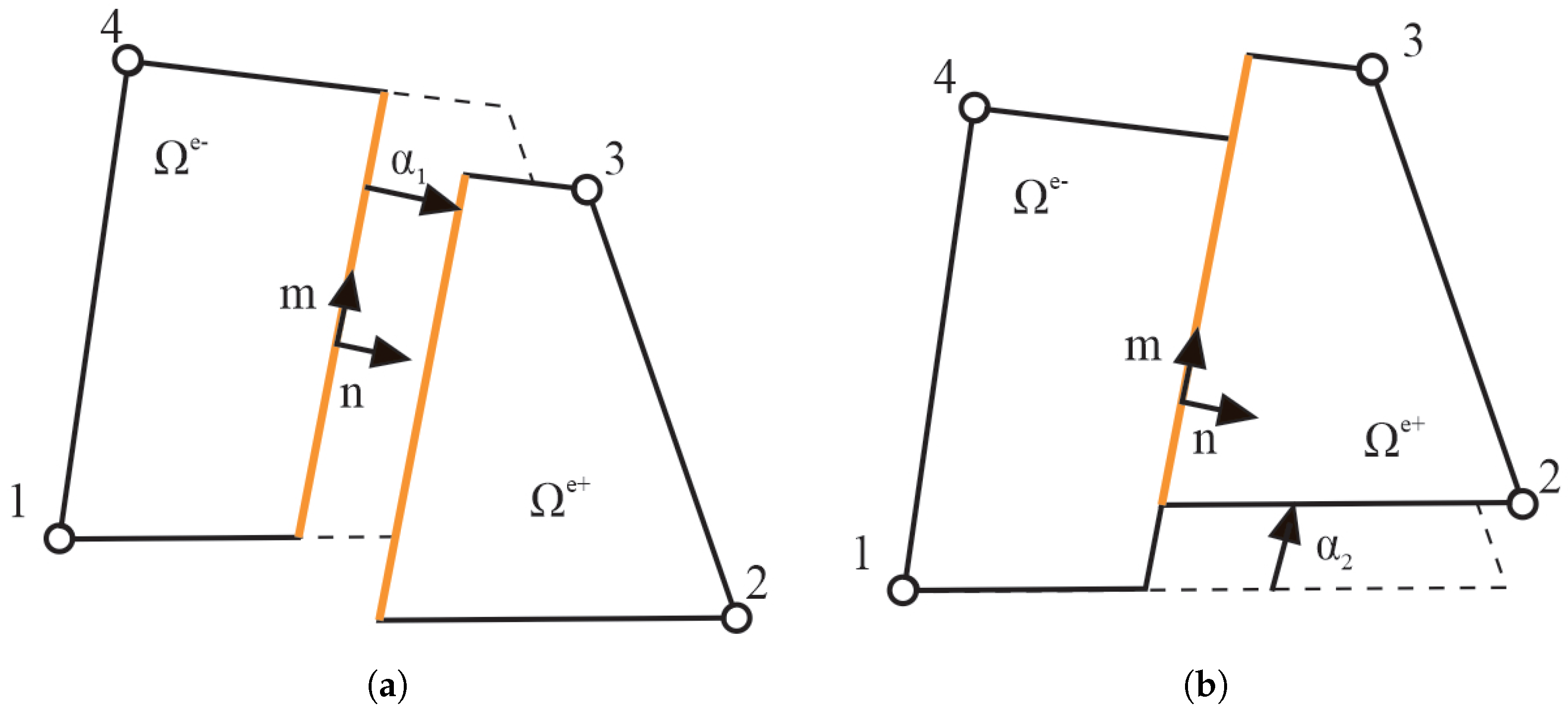
The crack embedding follows the statically and kinematically optimal nonsymmetric formulation (SKON) formulation of the embedded strong discontinuity method [48], which has demonstrated effectiveness in capturing complex fracture behaviors in materials [10]. In this approach, the crack inside each finite element is represented by a local jump in the displacement field over the defined crack line. This approach ensures that the results remain independent of the finite element size. Figure 1 illustrates the Q6ED finite element, which is capable of simulating the constant separation of material during cracking in both Mode I and Mode II. The separation of the material is controlled by softening parameters ${\alpha }_i$ (${\alpha }_1$ and ${\alpha }_2$).

As the crack is formed and keeps opening, the phenomenon of energy dissipation occurs. This phenomenon is defined by the exponential softening law and its internal variables ${\xi }_n$ and ${\xi }_m$. The values of the variables indicate the level of element degradation for both separation modes.

2.2. Kinematics

The quadrilateral finite element formulation is enhanced by incompatible modes and embedded discontinuities methods. The resulting displacement field is defined as follows:

$$\mathbf{u}(\xi ,{\Gamma }^e)=\sum _{a=1}^4{\mathbf{N}}_a\left(\xi \right){\mathbf{d}}_a+\sum _{b=1}^2{\mathbf{M}}_b\left(\xi \right){\rho }_b+\sum _{i=1}^2{\mathbf{p}}_i(\xi ,{\Gamma }^e){\mathbf{\alpha }}_i.$$

(1)

The first term represents the standard finite element part, where $N_a$ bilinear Lagrange interpolation functions and ${\mathbf{d}}_a$ are nodal displacement values. The second term introduces enhancements through the incompatible mode method, defined through the $M_1=1-{\xi }^2$ and $M_2=1-{\eta }^2$ shape functions and corresponding incompatible mode parameters ${\mathbf{\rho }}_b$. The last term accounts for embedded discontinuities, where ${\mathbf{p}}_i$ are discontinuity shape functions which are defined by assuming that during the fracture, ${\Omega }^{e-}$ part of the element remains still while the counterpart ${\Omega }^{e+}$ moves (see Figure 1):

$${\mathbf{p}}_1=\left(H_{\Gamma }\left(\mathbf{x}\right)\sum _{a\in {\Omega }^{e+}}{N}_a\right)\mathbf{n}{\mathbf{p}}_2=\left(H_{\Gamma }\left(\mathbf{x}\right)-\sum _{a\in {\Omega }^{e+}}{N}_a\right)\mathbf{m}.$$

(2)

The unit normal and tangent vectors to the crack ${\Gamma }^e$ from Equation (2) are represented by $\mathbf{n}={[n_x,n_y]}^T$ and $\mathbf{m}={[m_x,m_y]}^T={[-n_y,n_x]}^T$. The function $H_{\Gamma }$ represents the Heaviside step function, which introduces a displacement jump across the crack for $\mathbf{x}\in {\Omega }^{e+}$.

2.3. Crack Nucleation

The nucleation of cracks within each Q6ED element is governed by the stress state at the element’s four integration points, which determine both the crack’s location and orientation. The procedure, first introduced by [10], consists of two key processes: the fracture initiation and the definition of crack position and orientation.

Fracture initiation is regulated using the Rankine criterion, which assumes that a crack forms when the maximum principal stress exceeds the material’s tensile strength. At each simulation timestep, all uncracked finite elements are evaluated using this criterion. First, the principal stress values ${\sigma }_{p1,p2}^{e,i}$ at the four integration points are computed. The maximum principal stress at each integration point is determined by ${\sigma }_p^{e,i}=max[{\sigma }_{p1}^{e,i},{\sigma }_{p2}^{e,i}]$. The highest value among these is selected ${\sigma }_p^e=\underset{i=1,...,4}{max}{\sigma }_p^{e,i}$. This value is then compared with the tensile strength of the material ${\sigma }_n$. If ${\sigma }_p^e$ exceeds this value, the element fractures, and a crack within the element is initiated.

Once a crack is initiated, its position and orientation need to be defined. The integration points where ${\sigma }_p^e$ reaches its maximum value (within a tolerance) are collected in the set: $B^e=id\in 1,2,3,4:{\sigma }_p^{e,id}={\sigma }_p^e$. The geometric center of the crack is obtained by averaging the global coordinates of the points in $B^e$:

$${\mathbf{x}}_{ED}^e={\displaystyle \frac{1}{N_{B^e}}}\sum _{i\in B^e}{\mathbf{x}}^{e,i},$$

(3)

where $N_{B^e}$ is the number of contributing points, and ${\mathbf{x}}^{e,i}$ are their global coordinates. The average stress at points $B^e$ is calculated as follows:

$${\mathit{\sigma }}_{ED}^e={\displaystyle \frac{1}{N_{B^e}}}\sum _{i\in B^e}{\mathit{\sigma }}^{e,i},$$

(4)

where ${\mathit{\sigma }}^{e,i}$ are the stress values of each contributing point. The crack orientation angle ${\alpha }_{ED}^e$ is then derived from these averaged stress values:

$${\alpha }_{ED}^e={\displaystyle \frac{1}{2}}\arctan \left({\displaystyle \frac{2{\sigma }_{xyED}^e}{{\sigma }_{x{x}_{ED}}^e-{\sigma }_{y{y}_{ED}}^e}}\right).$$

(5)

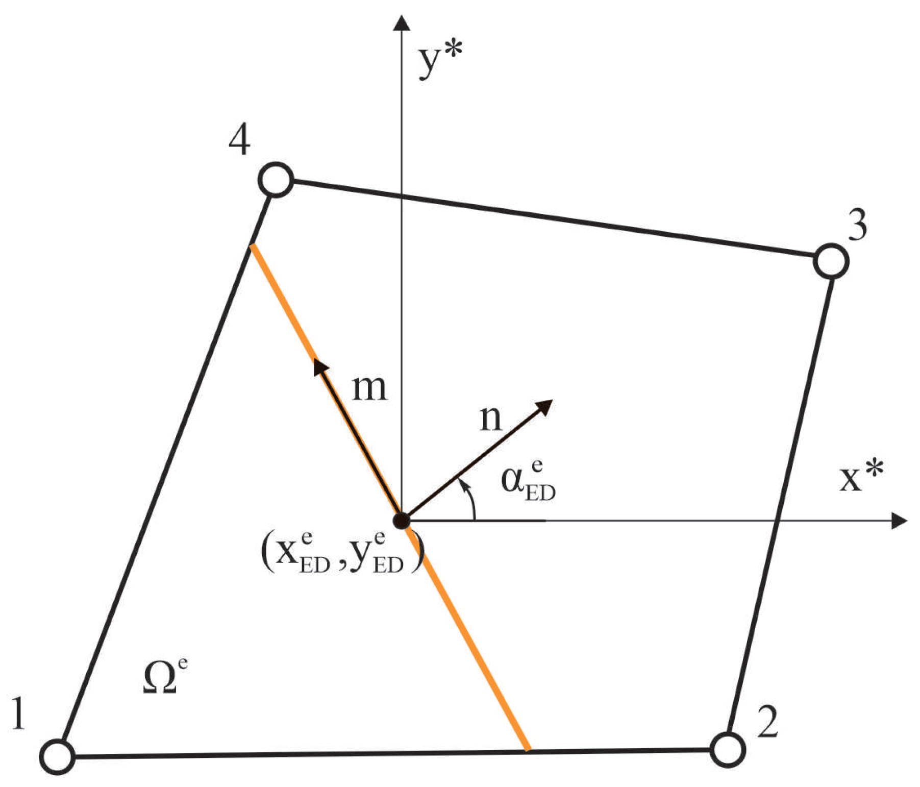
With the calculated position ${\mathbf{x}}_{ED}^e$ and orientation ${\alpha }_{ED}^e$, embedding the crack is straightforward (see Figure 2). The crack normal, represented by the angle ${\alpha }_{ED}^e$, aligns with the vector $\mathbf{n}$, while the tangential vector $\mathbf{m}$ is perpendicular to it. Once defined, the crack’s geometry remains fixed throughout the simulation, with only the separation parameters (${\alpha }_1,{\alpha }_2$) evolving over time. Each finite element can have only one crack, but multiple cracks can emerge across the mesh during each timestep.

2.4. Constitutive Law

The material initially deforms elastically, following the principles of Hooke’s law. The linear elastic behavior is applied to the bulk region of the element, where the stress is defined as $\mathit{\sigma }=\mathit{C}\overline{ϵ}$. Here, $\mathit{C}$ represents the constitutive matrix, determined by Young’s modulus E and Poisson’s ratio $\nu$, while $\overline{ϵ}$ denotes the strain in the bulk material.

During the loading process, each finite element is evaluated for elastoplastic behavior with isotropic hardening. At every Gaussian integration point, the equivalent stress is calculated based on the von Mises yield criterion:

$${\sigma }_{eq}=\sqrt{{\sigma }_{xx}^2+{\sigma }_{yy}^2-{\sigma }_{xx}{\sigma }_{yy}+3{\tau }_{xy}^2}.$$

(6)

The corresponding yield function is defined as follows:

$$f={\sigma }_{eq}-\left({\sigma }_0+H·{\epsilon }_p^{*}\right),$$

(7)

where ${\sigma }_0$ is the yield strength, H is the hardening modulus, and ${\epsilon }_p$ is the equivalent plastic strain for each Gauss integration point. If the yield function returns a positive value, elastoplastic isotropic hardening occurs at that integration point. The plastic strain is then updated using the radial return algorithm (see [1]), and the stress tensor is subsequently computed as follows: $\sigma =\mathit{C}(\overline{ϵ}-{ϵ}_p)$, where ${ϵ}_{\mathit{p}}$ represents the plastic strain tensor.

As the stress continues to increase and surpasses the material strength, the first cracks begin to form. At this phase, the finite element is divided into the crack domain and the remaining bulk material. Crack behavior, including material degradation and energy dissipation, is governed by two uncoupled plasticity softening laws [1]. Each law corresponds to the separation modes, Mode I (opening) and Mode II (sliding), and is formulated within the framework of thermodynamics using Helmholtz free energy. These laws describe the dissipation of energy during the fracture process of material by irreversible accumulation of plastic deformations while preserving the stiffness of the material.

When the Rankine failure criterion is activated, the softening failure function $\overline{\overline{\varphi }}$ controls the material degradation and evolution of internal variables. For tensile Mode I, it is defined as follows:

$${\overline{\overline{\varphi }}}_n(t_1,{\overline{\overline{q}}}_n)=t_1-({\sigma }_n-{\overline{\overline{q}}}_n)\le 0,$$

(8)

where $t_1$ is the normal traction value on the crack line and ${\sigma }_n$ is the material tensile strength. The variable ${\overline{\overline{q}}}_n$ represents the softening traction value:

$${\overline{\overline{q}}}_n={\displaystyle \frac{\partial {\overline{\overline{\Psi }}}_n}{\partial {\overline{\overline{\xi }}}_n}}={\sigma }_n\left(1-exp\left[-{\displaystyle \frac{{\sigma }_n}{G_{fn}}}{\overline{\overline{\xi }}}_n\right]\right),$$

(9)

where $G_{fn}$ is the Mode I material fracture energy and ${\overline{\overline{\xi }}}_n$ is the internal softening variable.

For shear Mode II, Equation (9) remains valid, with the notation changed from n to m to represent Mode II parameters. The failure function for shear Mode II is formulated as follows:

$${\overline{\overline{\varphi }}}_m(t_2,{\overline{\overline{q}}}_m)=\left|t_2\right|-({\sigma }_m-{\overline{\overline{q}}}_m)\le 0.$$

(10)

Here, $t_2$ represents the tangential traction on the crack line, and its absolute value is related to the potential for the crack to slide in both directions.

With the constitutive laws defined, the entire fracture process of the material in the Q6ED model is determined by the previously introduced elastic, elastoplastic and fracture model parameters. Since this paper deals with only tensile fracture of the material, shear fracture parameters are neglected. So, uncertain parameters subjected to the identification procedure can be collected into a single vector $\mathbf{z}$:

$$\mathbf{z}=\left[E,\nu ,{\sigma }_0,H,{\sigma }_n,G_{fn}\right]$$

(11)

3. Bayesian Model Calibration

Material failure is a complex, nonlinear process governed by constitutive laws and their corresponding input parameters, which play a crucial role in simulations by influencing both crack initiation and propagation. Accurately determining these parameters is essential for achieving reliable simulation outcomes.

This work relies on minimizing the discrepancy between numerical model predictions and experimental observations by using simple measurements such as those shown in [49]. The relationship between the parameters $\mathbf{z}$ and measurable test behavior is expressed as follows:

$$\mathbf{u}=\mathcal{G}\left(\mathbf{z}\right)\mathbf{u}\in {\Re }^Q.$$

(12)

Here, $\mathbf{u}$ represents the vector of measurable model outputs, and $\mathcal{G}$ denotes the numerical model operator, often referred to as the forward model, that predicts these measurements based on the values of model parameters $\mathbf{z}$. The objective of identification is to determine the optimal values of $\mathbf{z}$ such that the model output $\mathbf{u}$ closely matches observed data. This leads to an inverse problem, where the forward model $\mathcal{G}$ must be inverted to estimate the unknown parameters accurately. This section provides a brief overview of probabilistic Bayesian inverse method used in this work, along with its accompanying methodology. For more details, refer to [49].

3.1. The Bayesian Inverse Method

The Bayesian inverse method is a robust and efficient probabilistic approach for identifying uncertain parameter values by solving the inverse problem. In this work, the uncertain parameters are defined in Equation (11). These parameters are treated as random variables and are expressed in vector form as $\mathbf{z}:\Omega \to {\mathbb{R}}^n$

$$\mathbf{z}\left(\omega \right):=\left[E\left(\omega \right),\nu \left(\omega \right),{\sigma }_0\left(\omega \right),H\left(\omega \right),{\sigma }_n\left(\omega \right),G_{fn}\left(\omega \right)\right],$$

(13)

where $\omega$ represents one realization from the set of all possible realizations $\Omega$. Each model parameter $z_i$ within the vector $\mathbf{z}$ is described by its probability density function $\pi \left(z_i\right)$. Assuming that the input parameters are mutually independent, their joint probability function $\pi \left(\mathbf{z}\right)$ can be expressed as [23,50]:

$$\pi \left(\mathbf{z}\right)=\pi (z_1,\dots ,z_{N_i})=\prod _{i=1}^{N_i}{\pi }_i\left(z_i\right).$$

(14)

The term $\pi \left(\mathbf{z}\right)$ is referred to as the prior distribution of the parameter values. The selection of the prior distribution is influenced by various factors, including prior experience, results from previous identification efforts, available measurement data, or even mere assumptions [23,50].

The solution of the numerical forward model, $\mathcal{G}$, with the “true” set of input parameters should ideally match the obtained measurements from the analyzed structure or specimen. However, in practice, this is not achievable due to inherent errors and imperfections in both the measurement and modeling processes, especially when dealing with nonlinear phenomena. Taking this into account, an obtained measurement ${\mathbf{d}}_m$ can be expressed as a realization of a random variable [23,50]:

$${\mathbf{d}}_m\left({\omega }_e\right)={\mathbf{u}}_{\mathrm{true}}+ϵ\left({\omega }_e\right)=\mathcal{G}\left({\mathbf{z}}_{\mathrm{true}}\right)+ϵ\left({\omega }_e\right).$$

(15)

Here, ${\mathbf{u}}_{\mathrm{true}}$ represents the measurable variable predicted by using the “true” parameter values ${\mathbf{z}}_{\mathrm{true}}$, while $ϵ$ accounts for the the combined errors in the measurement and the modeling, depending on the specific realization ${\omega }_e$. These errors are described by their probability density function ${\pi }_{ϵ}$. It is further assumed that the realizations of the errors $\mathit{ϵ}$ are independent of the realizations of the uncertain input parameters $\mathbf{z}$, ensuring that the random variables $\mathbf{z}$ and $\mathit{ϵ}$ are independent. Accurately defining the error distribution is a crucial step in the identification process. This work considers three types of additive errors: measurement errors, numerical model errors, and proxy modeling errors

$$\mathit{ϵ}={\mathit{ϵ}}_{\mathrm{meas}}+{\mathit{ϵ}}_{\mathrm{model}}+{\mathit{ϵ}}_{\mathrm{proxy}},$$

(16)

where the last term, ${\mathit{ϵ}}_{\mathrm{proxy}}$, arises when the computationally expensive numerical simulation is replaced by a proxy model. These three error components are assumed to be mutually independent.

The measurement error ${\mathit{ϵ}}_{\mathrm{meas}}$ is often assumed to follow a normal distribution, ${\mathit{ϵ}}_{\mathrm{meas}}\sim \mathcal{N}(\mathbf{0},{\mathbf{C}}_{\mathrm{meas}})$, centered around the experimental measurements. This assumption is justified by the use of standardized calibration and testing procedures, which ensure consistent and reliable measurement performance. The covariance matrix ${\mathbf{C}}_{\mathrm{meas}}$ is taken as diagonal, assuming independent error components. The diagonal entries ${\sigma }_i^2$ are defined based on the manufacturer’s specifications of the measurement device, which may be expressed as a percentage of the measured values. This percentage typically reflects the maximum possible error, which is here interpreted as a $3{\sigma }_i$ deviation under the normal distribution assumption. Consequently, the standard deviation ${\sigma }_i$ of the measurement error is calculated by dividing the maximum error by three.

In contrast, modeling and proxy errors are inherently more complex. They may exhibit correlation, systematic bias, or non-Gaussian behavior, especially near crack initiation. If not properly addressed, such simplifications can lead to underestimated uncertainties and biased parameter estimates, even if the model fits the experimental data. Various strategies exist to handle numerical model errors. One approach is to treat the associated covariance matrix as an additional unknown within the identification process [25]. Alternatively, it can be estimated separately as a deterministic, input-dependent function, based on the constitutive laws employed and comparisons between model predictions and experimental data. To avoid the risk of incorporating incorrectly estimated bias and correlations, a simple analysis was conducted comparing model predictions with experimental results for non-linear data. This revealed that modeling error exhibited noticeable bias only in the later stages of testing, where increased uncertainty was already anticipated. In contrast, proxy model errors were generally small and only weakly correlated, with a negligible impact on the later parts of the response. Based on these findings, we adopt the simplifying assumption that these error components are also zero-mean, mutually independent, and Gaussian. This is considered a pragmatic compromise in the absence of reliable bias quantification. Thus, the modeling errors ${\mathit{ϵ}}_{\mathrm{model}}$ were modeled as heteroscedastic measurement noise, where the variance is an input-dependent function of the chosen quantities. For the proxy modeling error ${\mathit{ϵ}}_{\mathrm{proxy}}$, the standard deviation is estimated from the variance of proxy errors evaluated on an independent validation dataset, i.e., input–output pairs not used during proxy model training.

The main idea of the Bayesian method is to update the prior distribution of the parameters $\pi \left(\mathbf{z}\right)$ using the obtained measurements ${\mathbf{d}}_m$ by applying Bayes’ theorem of conditional probability [23,51,52]:

$$\pi \left(\mathbf{z}\right|{\mathbf{d}}_m)={\displaystyle \frac{\pi \left({\mathbf{d}}_m\right|\mathbf{z})\pi \left(\mathbf{z}\right)}{\pi \left({\mathbf{d}}_m\right)}}.$$

(17)

Here, $\pi \left({\mathbf{d}}_m\right|\mathbf{z})$ represents the likelihood function, which quantifies the probability of obtaining the measurement ${\mathbf{d}}_m$ given a specific set of parameter values $\mathbf{z}$. This likelihood function is defined by the probability that the error $ϵ$ equals ${\mathbf{d}}_m-\mathbf{u}$ [23], where $\mathbf{u}$ is computed from the forward operator $\mathbf{u}=\mathcal{G}\left(\mathbf{z}\right)$.

The term $\pi \left({\mathbf{d}}_m\right)$ is referred to as the evidence function. It serves as a normalization constant in Bayes’ theorem, ensuring that the posterior distribution $\pi \left(\mathbf{z}\right|{\mathbf{d}}_m)$ integrates to 1.

The expression $\pi \left(\mathbf{z}\right|{\mathbf{d}}_m)$ represents the posterior distribution of the parameter values $\mathbf{z}$. This distribution is the final result of the Bayesian inverse procedure, representing the updated understanding of the parameter values based on the used measurements ${\mathbf{d}}_m$.

A common challenge with the Bayesian inverse method is that, in most cases, the posterior distribution cannot be formulated explicitly. To address this, various mathematical techniques, such as sampling methods, have been developed to approximate its shape.

Sampling methods generate samples that approximate a stationary distribution matching the desired posterior distribution. In this work, the Markov Chain Monte Carlo (MCMC) method, based on the Metropolis–Hastings algorithm, is chosen as a robust, simple, and model-independent technique [19,50,51,53,54]. This method employs a random walk approach to efficiently generate samples from the posterior distribution.

However, when the posterior distribution exhibits a complex shape, the effective application of the MCMC method requires evaluating hundreds or even thousands of proposed parameter candidates. The most computationally intensive part of this process is constructing the likelihood function, which involves computing the forward model solutions $\mathcal{G}\left(\mathbf{z}\right)$ for each candidate parameter. For complex numerical models, such as models to simulate fracture processes, this represents a significant computational burden. To mitigate this, mathematical proxy models are often employed.

3.2. General Polynomial Chaos Expansion (gPCE) Proxy Model

Performing multiple fracture simulations often requires extensive computational efforts, which can be both time and resource-consuming. These can make solving the Bayesian inverse problem using the MCMC method excessively slow or even impossible. To address this issue, mathematical proxy models are necessary. These models, also known as surrogate, meta, or response surface models, provide approximate results of numerical simulations with a certain degree of precision, thereby significantly accelerating the computational process [51,55,56]:

$$\mathcal{G}\left(\mathbf{z}\right)\approx \tilde{\mathcal{G}}\left(\mathbf{z}\right).$$

(18)

Here, $\tilde{\mathcal{G}}\left(\mathbf{z}\right)$ represents the proxy model’s approximation of the forward model operator $\mathcal{G}$.

The choice of proxy model must be made carefully, taking into account the characteristics of the analyzed problem. The study [49] compares the accuracy of various proxy models used to approximate numerical simulation results in crack propagation problems. With respect to performance, for simpler fracture propagation cases, the gPCE model demonstrated accuracy comparable to other approaches, such as neural networks, and was effective in achieving precise parameter identification. From a practical standpoint, the gPCE model is well-regarded for its computational efficiency and ease of training. Additionally, a sufficiently accurate gPCE model provides an analytical representation of the numerical model’s output, enabling efficient statistical analysis with minimal computational cost. Based on these considerations, the gPCE proxy model is selected. However, it is important to note that for more complex fracture problems, gPCE may not be the most suitable proxy model, as highlighted in the same study.

The gPCE method approximates numerical model solutions through a linear combination of multidimensional polynomials and their corresponding coefficients [53,57,58], as expressed by the following:

$$\mathbf{u}=\mathcal{G}\left(\mathbf{z}\right)\approx \tilde{\mathcal{G}}\left(\mathbf{z}\right)=\tilde{\mathbf{u}}=\sum _{k=0}^{K-1}{\nu }_k{\Phi }_k\left(\mathbf{z}\right)={\rm Y}\Phi \left(\mathbf{z}\right),$$

(19)

where $\tilde{\mathbf{u}}$ represents the approximation of the numerical model’s output, $\Phi$ is the selected set of polynomials collected in the vector $\Phi ={[{\Phi }_0\left(\mathbf{z}\right),{\Phi }_1\left(\mathbf{z}\right),\dots ,{\Phi }_{K-1}\left(\mathbf{z}\right)]}^T$, and ${\rm Y}=[{\nu }_0,{\nu }_1,\dots ,{\nu }_{K-1}]$ denotes the coefficients of the polynomial expansion, where ${\nu }_k\in {\mathbb{R}}^Q$ corresponds to the polynomial ${\Phi }_k$.

To accurately approximate the forward model, a polynomial basis is first selected based on the prior distribution of the model parameters. The coefficients ${\rm Y}$ are then determined by solving a linear regression problem that minimizes the mean squared error (MSE) [53]:

$$\mathbb{E}\left[{\widetilde{ϵ}}^2\right]=\mathbb{E}\left[{(\mathbf{u}-\tilde{\mathbf{u}})}^2\right]={\int }_{\mathbb{R}}{(\mathbf{u}\left(\mathbf{z}\right)-\tilde{\mathbf{u}}\left(\mathbf{z}\right))}^2\pi \left(\mathbf{z}\right)d\mathbf{z}\approx {\displaystyle \frac{1}{N}}\sum _{i=1}^N\left(\mathbf{u}\left({\mathbf{z}}_i\right)-\tilde{\mathbf{u}}\left({\mathbf{z}}_i\right){)}^2\right).$$

(20)

One significant advantage of the gPCE method is its ability to compute sensitivities directly from its coefficients [59]. Sensitivity analysis plays an essential role in experimental design, helping to optimize sensor placement and identify the most informative measurable outputs [60]. In this study, we used Sobol Sensitivity Analysis, a method for evaluating the contribution of input variables (i.e., model parameters) to the variance in the model’s output. This method decomposes the total variance in the output into partial variances, which can be calculated directly from the coefficients of the gPCE model. Partial variance measures the extent to which the variability in the solutions $\mathit{u}$ can be attributed to the changes in the values of one or more model parameters. Sobol indices represent this relative measure by the ratio of partial variance (caused by variations in a specific subset of model parameters) to the total variance (resulting from all model parameters) [49,61,62,63].

4. Test Design and Experimental Setup

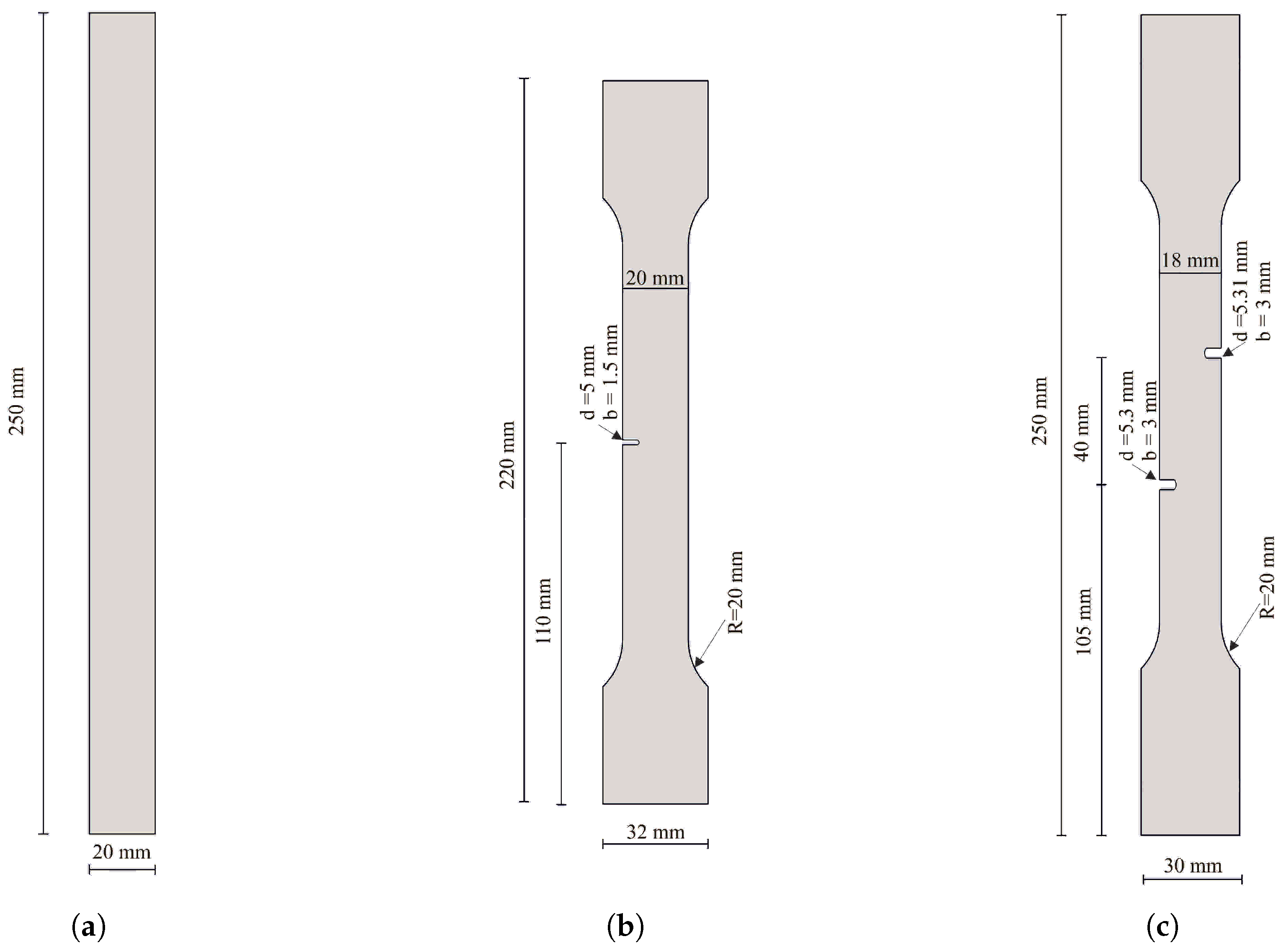
The identification of parameters was performed for aluminum 6060 alloy specimens with unknown properties through the tensile loading tests. Three different specimen designs were selected for the experiments (see Figure 3).

Before conducting physical experiments, it is important to carry out a test design procedure to evaluate the effectiveness of the planned tests, specimen geometries, and measurement techniques for identifying the target parameters. This helps reduce the risk of test failure. As a part of this process, sensitivity analysis is used to gain insights into how strongly different parameters influence the planned measurements. In this study, Sobol sensitivity analysis was applied to quantify the effect of parameter variations on the simulated responses. To support this, virtual simulations were created to replicate the planned experiments. By examining how different combinations of parameter values affect the measured responses, the most informative measurements and configurations can be selected. Following the sensitivity analysis, the chosen measurements were applied in the laboratory in order to identify the uncertain parameters and to verify their results.

4.1. Test Design

The uncertain parameters of the aluminum alloy are treated as random variables, initially characterized by a uniform prior distribution $z_i\sim \mathcal{U}(a,b)$. This choice reflects a non-informative prior defined between the bounds given based on the best engineering judgment. These bounds are given in

Table 1. Prior distributions for material parameters.

Parameter	Distribution	Left Bound (a)	Right Bound (b)
E	$U(a,b)$	$50,000\mathrm{N}/{\mathrm{mm}}^2$	$100,000\mathrm{N}/{\mathrm{mm}}^2$
$\nu$	$U(a,b)$	$0.2$	$0.4$
${\sigma }_0$	$U(a,b)$	$50\mathrm{N}/{\mathrm{mm}}^2$	$150\mathrm{N}/{\mathrm{mm}}^2$
H	$U(a,b)$	$2000\mathrm{N}/{\mathrm{mm}}^2$	$6000\mathrm{N}/{\mathrm{mm}}^2$
${\sigma }_n$	$U(a,b)$	$150\mathrm{N}/{\mathrm{mm}}^2$	$300\mathrm{N}/{\mathrm{mm}}^2$
$G_{fn}$	$U(a,b)$	$100\mathrm{N}/\mathrm{mm}$	$300\mathrm{N}/\mathrm{mm}$

. The parameter identification process is conducted in two phases. In the first phase, the rectangular specimen (see Figure 3a) is used to identify the elastic parameters (E and $\nu$). Although Young’s modulus E and Poisson’s ratio $\nu$ are standard parameters in engineering, for stochastic computations, it is often more advantageous to work with the bulk modulus K and shear modulus G, as they directly correspond to the eigenvalues of the constitutive matrix. Ensuring the positivity of K and G automatically guarantees the positive definiteness of the constitutive matrix. Nevertheless, in this work, we use the parameter pair $(E,\nu )$, and enforce the positivity of K and G through appropriately bounded distributions of these parameters.

The proposed laboratory setup for parameter identification includes both force−displacement measurements and deformation measurements taken from the specimen’s lateral surfaces. In the middle of the specimen, two points were selected on opposite sides of the lateral boundary, and the sum of their horizontal displacements is used as a measurement. To validate the feasibility of this approach prior to experimental testing, a Sobol sensitivity analysis was performed. A set of 200 parameter combinations from the prior distribution was generated using a Quasi-Monte Carlo (QMC) sampling technique, ensuring a well-distributed sample set. For each generated sample, virtual measurements were collected at different time steps using a linearly incrementing displacement control. Then a gPCE model was trained using 150 random samples, while 50 were used for accuracy testing. The degree of the polynomial basis was optimized to achieve the best accuracy. The results of the sensitivity analysis, presented in Figure 4, confirm that the selected measurements effectively capture the influence of both elastic parameters.

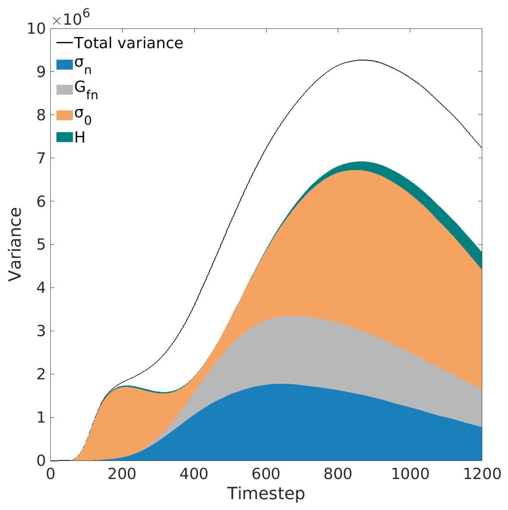
For the identification of the elastoplastic hardening and fracture parameters, the single−notched dog bone specimen is used (see Figure 3b). For this case, only a force−displacement measurement was selected for the identification process. Following the same procedure as the elastic parameter identification, a set of 2000 combinations of parameters was generated using QMC sampling and a corresponding gPCE model was trained. The results, presented in Figure 5, show that force−displacement measurement is sufficient to capture the influences of the elastoplastic and fracture model parameters.

4.2. Experimental Setup

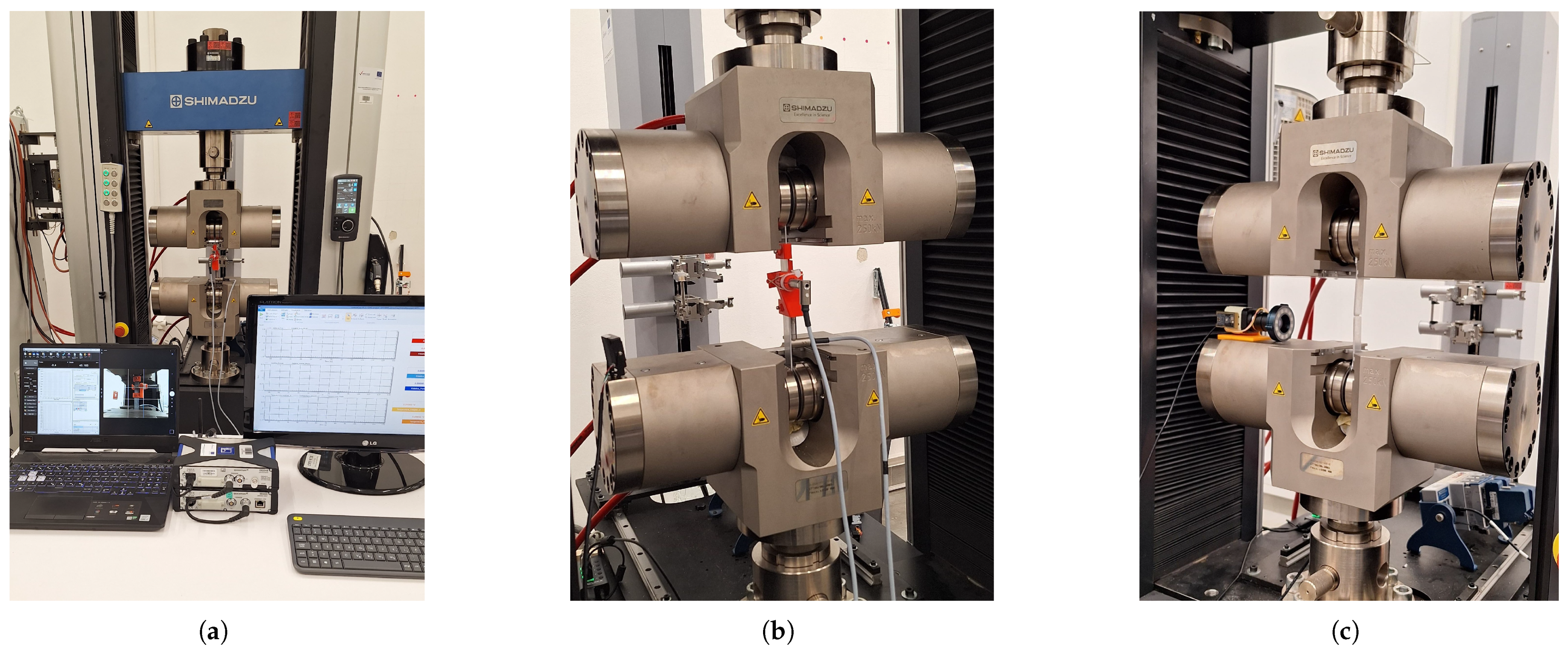
Experimental investigations were conducted in the Structures Laboratory of FCEAG at the University of Split. Multiple measurement systems were used to obtain precise data on the physical properties of the test specimens (see Figure 6). The samples were fabricated from 6060 T4 aluminum alloy stock using a CNC milling machine, in accordance with the ISO 6892 standard. Additionally, some of the specimen was notched to induce stress concentration areas, as illustrated in Figure 3. Dimensional accuracy was verified prior to every test.

Specimens were loaded using a Shimadzu AGX-V 250 kN Universal Testing Machine (UTM), Shimadzu, Singapore. Strains were measured with an SIE extensometer and a crossbar positional sensor; both devices are classified as accuracy class 0.5. Forces were recorded using a load cell (nominal capacity 250 kN, accuracy class 0.5). Testing was performed under displacement control of the upper jaw at a constant speed of 2 mm/min, chosen to match the strain rate from ISO 6892. The termination condition was defined as a 10% drop in subsequent force, and data were sampled at 100 Hz.

To determine Poisson’s ratio, additional sensors and measurement systems were utilized. Longitudinal and transverse strains were measured using LVDT sensors (HBM WA-L, 0–10 mm nominal range). A custom made 3D-printed jig, manufactured from ABS plastic on a BambuLab X1Carbon desktop 3D printer, was used to hold the sensors orthogonally and maintain attachment to the sample during loading. The testing regime for measuring Poisson’s ratio was limited to the elastic deformation region and cycled five times before data collection to ensure the positional stability of all components in the measurement chain. The LVDT sensors were connected to an HBM Quantum MX840B universal amplifier, which acquired data independently of the UTM. To synchronize the two data sources (the UTM and the MX840B), analog signals representing crossbar displacement and force were recorded by the MX840B.

In addition to the mechanical measurements, an optical measurement system was employed. An industrial camera (2560 × 1440 pixels) was positioned with its imaging plane parallel to the specimen plane and configured to capture an image every 0.5 s. It was synchronized with the data acquisition software so that crossbar displacement and force values were recorded for each frame. The camera used a varifocal lens (5–50 mm) with a maximum aperture of f/1.6. Captured images were undistorted to remove radial and tangential distortions using camera parameters obtained through a checkerboard calibration procedure; this step was repeated for every experimental setup to account for the variable zoom setting. Camera parameter determination and image undistortion were carried out in MATLAB (version 9.13.0, R2022b, The MathWorks Inc.: Natick, MA, USA, 2022).

A random speckle pattern was applied to the samples to facilitate Digital Image Correlation (DIC). The DIC analysis was performed using the open-source software [64], implemented in the MATLAB environment [65].

To assess the accuracy of the DIC system, a calibration run was carried out. Before each tensile test, the specimen was translated through the camera’s field of view using the UTM crossbar. The sample was held only by the upper jaw, leaving the lower end free. The position of the sample was recorded using the MX840B amplifier. Analysis of the calibration run revealed displacement accuracy and apparent strain values related to lens irregularities, specimen preparation, and DIC limitations. The root-mean-square error in displacement was 0.1 mm, and the strain noise was below $1\times {10}^{-3}$, primarily due to camera limitations (and to a lesser extent, specimen preparation and inherent DIC constraints). Nevertheless, the DIC data were qualitatively accurate in capturing the expected strain distributions near critical stress zones.

A summary of the identification procedures for elastic, elastoplastic, and fracture parameters—along with details on specimen types, measurement methods, and equipment used—is provided in

Table 2. Identification of elastic, elastoplastic, and fracture parameters.

Parameter	Specimen	Measurement	Equipment
E	Rectangular	Force−displacement	UTM
$\nu$	Rectangular	Lateral deformation	LVDT
${\sigma }_0,H,{\sigma }_n,G_{fn}$	Single−notched	Force−displacement	UTM

.

5. Results

This section presents the results of the Bayesian identification process for the uncertain parameters of aluminum 6060 alloy specimens. The identification was performed using experimental measurements in conjunction with a trained generalized Polynomial Chaos Expansion (gPCE) proxy model, developed from virtual test data, and a Markov Chain Monte Carlo (MCMC) analysis within a Bayesian framework. The numerical simulations were implemented within the FEAP finite element framework [66], while the gPCE model training and MCMC sampling were carried out using the open-source library SGLIB [67].

To ensure consistency with the experimental setup, the virtual tests used for training the proxy model were designed to replicate the same boundary conditions and loading rates. Virtual measurements were gathered from a timestep-based simulation, where each timestep represents every tenth data point collected by the measurement equipment. This discretization yields 590 timesteps for measurement regarding the identification of the elastic parameters and 1200 timesteps for the elastoplastic and fracture ones. All virtual test simulations were executed on a high-performance cluster computer, which is capable of running 400 parallel computations.

5.1. Identification of Elastic Parameters

The identification process begins with the training of a proxy model to ensure a fast yet precise approximation of virtual test results of the numerical model. To train the gPCE proxy model, a dataset of 800 parameter combinations was generated from the prior distribution using QMC sampling, with an additional set of 200 for accuracy testing. The computation of the results for this parameter sample by cluster computer took around 5 min to complete. Training the optimal gPCE model involves solving Equation (20) and selecting the polynomial degree that minimizes the error metrics between the proxy model and the generated test sample results from the numerical model. In this work, the mean Maximum Absolute Error (MAE) averaged over the timestep domain is used. A fourth-degree polynomial with 15 coefficients per timestep was found to provide the best fit.

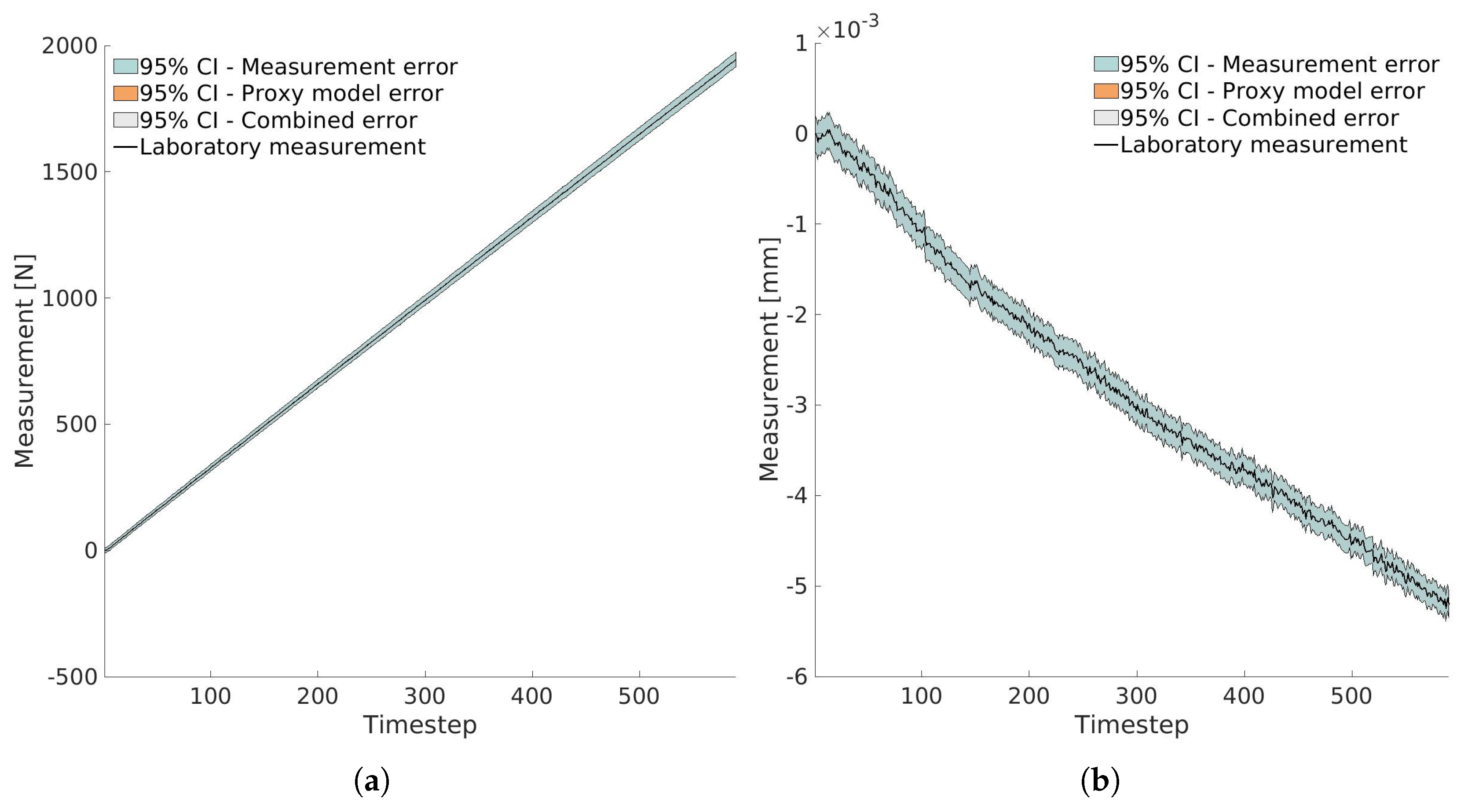
With the trained proxy model, the next step is to define the error distributions. First, we consider the measurement error distribution. For the force–displacement data, the standard deviation ${\sigma }_i$ is set to 0.167% of the measured value. This is based on the maximum error specified by the UTM machine (class 0.5), assuming the maximum error represents $3\sigma$ under a normal distribution. For the lateral deformation measurements, the standard deviation is determined in the same way using the error specified by the LDTV manufacturer (class 0.5), and is also set to 0.167% of the measured value. Additionally, a constant component of $0.0001\mathrm{mm}$ is included to account for other sources of noise, such as those originating from the measuring circuitry, thermal fluctuations, and similar effects, which manifest as spikes due to the small magnitude of measured values (see Figure 7b).Since the identification of elastic parameters focuses on the material’s linear elastic behavior, modeling errors are not considered at this stage. The constitutive law used in the numerical model is sufficiently accurate for this purpose. The standard deviation of the proxy model error is defined based on the differences between the predictions of the trained gPCE model and the results obtained from 200 independent testing samples. These error distributions, along with the collected laboratory measurements, are presented in Figure 7. Here, only the measurement errors are visible, as the proxy model errors are very small due to the linear nature of the problem.

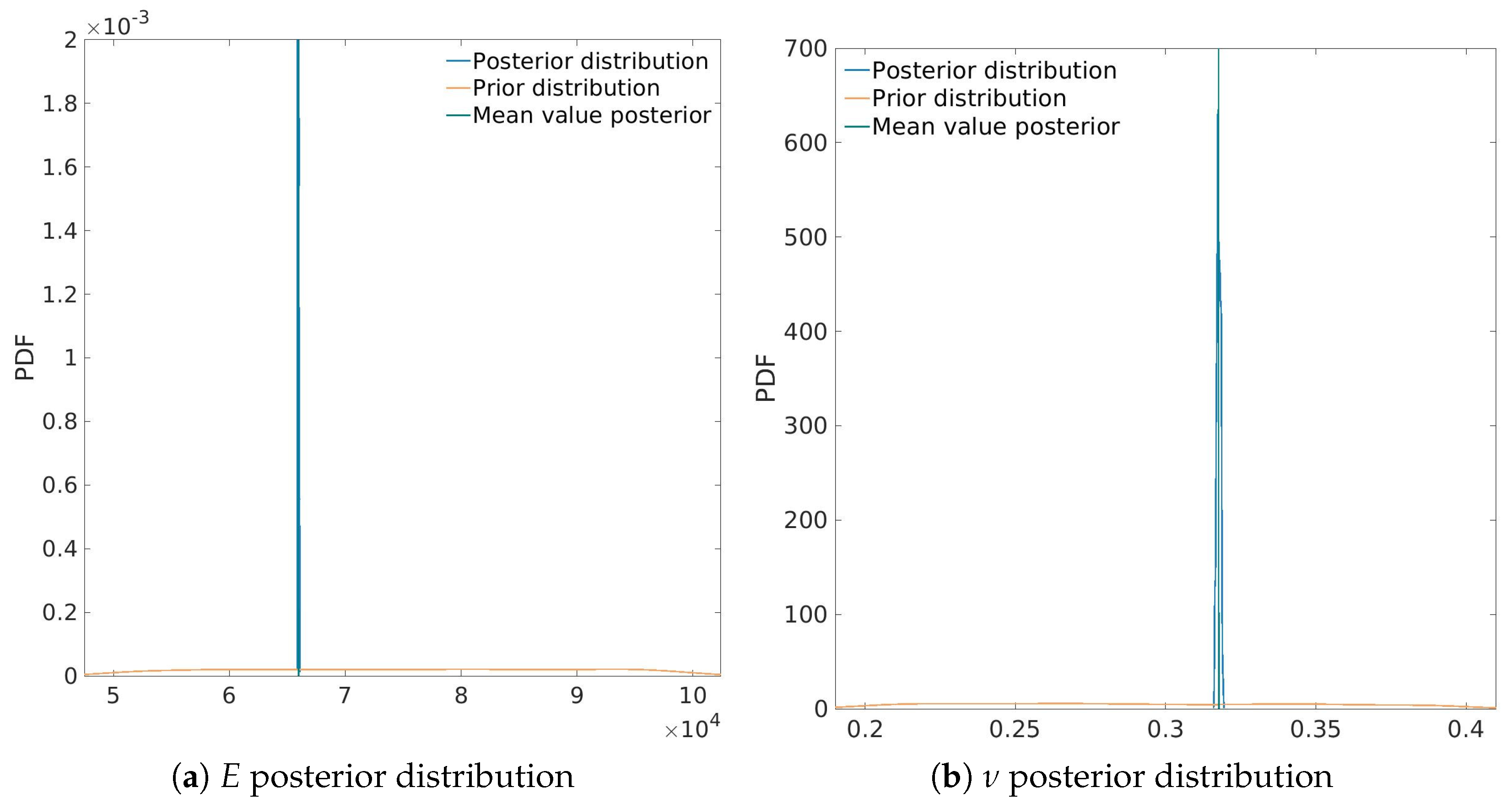
The MCMC analysis is conducted using 100 Markov chains and 500 simulation steps, totaling 50,000 computed results for the combinations of the elastic parameters. The entire analysis was completed in less than a minute. The results of the identification are shown in Figure 8. The results shows a successful identification of both elastic parameters, as their posterior distributions have minimal variation, which ensures a high degree of certainty. The maximum a-posterior (MAP) value—the point estimate of the parameter, maximizing the posterior distribution—for Young’s modulus E is 66,542 N/mm², while the Poisson’s ratio $\nu$ is 0.319. These values are considered certain and are used as constants in the next phase of the identification.

5.2. Identification of Elastoplastic and Fracture Parameters

This phase of the identification process involves the elastoplastic hardening of the material, the development of microcracks, the formation of the macrocrack, and finally, the material failure. These processes result in complex datasets that are much more challenging to interpret compared to elastic parameters, resulting in significantly higher computational effort needed.

To train the gPCE model, 20,000 samples were generated from the prior distributions using QMC sampling, with an additional 5000 samples used for testing. These computations performed on a cluster computer required approximately 70 h to complete. After validation and testing, a ninth-degree polynomial gPCE with 715 coefficients per timestep was found to provide the most accurate results.

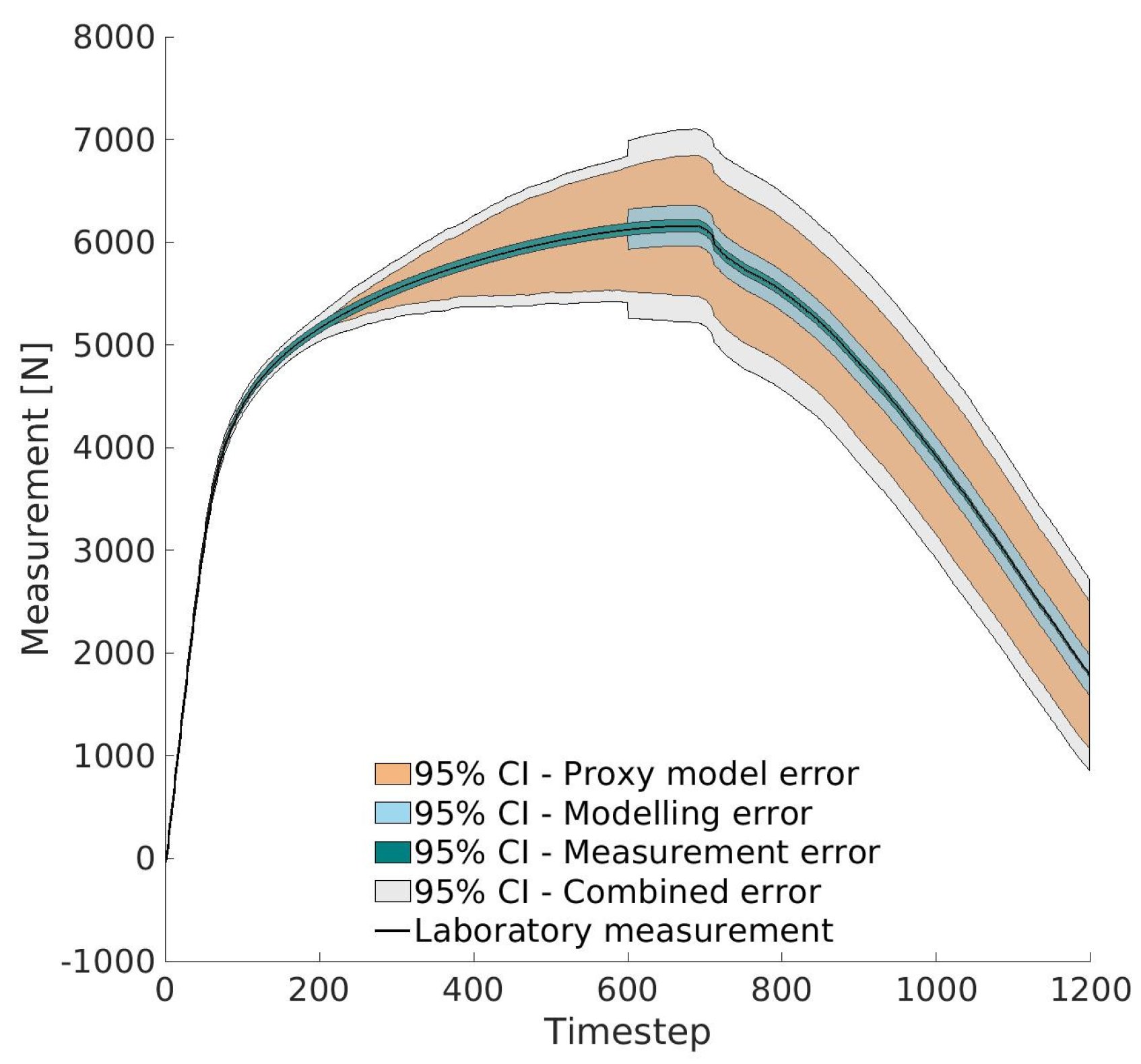
Regarding the definition of the error distributions, the standard deviation of the measurement error ${\sigma }_i$ was set to 0.167% of the measured value. The modeling error is defined by comparing the laboratory measurements with the results from the numerical model, based on knowledge of the constitutive laws used. Here, we divide the modeling error into two parts. The first part relates to the linear elastic and elastoplastic hardening behavior, as well as the onset of microcrack formation. For this part, a standard deviation of ${\sigma }_i=25$ N is chosen. This value is selected because the numerical model produces identical outputs for the same input parameters, whereas real materials exhibit inherent variations. Since the elastic parameters were fixed in the previous phase and by considering the small influence of the nonlinear behavior of microcracks, this error distribution is selected to cover potential variations. The second part of the modeling error relates to the merging of microcracks, the formation of macrocracks, and the final material failure. In the numerical model, energy dissipation is represented by an exponential softening law. However, this is only an approximation of a highly nonlinear real-world phenomenon. Given the potential for larger variations when sudden material failure occurs, the error distribution for this part is set to be significantly larger, with ${\sigma }_i=100$ N. Finally, the proxy model error is determined by comparing its predictions for the testing samples with the results from the numerical model. These error distributions, along with laboratory measurements, are presented in Figure 9.

The biggest error comes from the proxy modeling. This is primarily due to the complex and nonlinear nature of the problem, for which we have a complex, nonsmooth response surface that is difficult to approximate. Because a wide range of prior distributions was considered, the samples in the testing set exhibit substantial variation. At a given timestep, some samples remain in the linear elastic regime, others undergo elastoplastic hardening, some initiate cracking, and others may approach complete failure. Capturing such a diverse dataset is challenging for different proxy modeling techniques [49]. Therefore, when analyzing fracture propagation problems, it is inevitable that relatively larger errors will be encountered in proxy modeling. That is why it is important to include these errors inside the identification process through the error model to ensure that the uncertainty introduced by the proxy is properly reflected in the posterior distributions of the identified parameters.

One suggested strategy to reduce proxy modeling errors is to perform multiple iterations of the identification process for the same test. After the initial identification, the resulting posterior distributions can be broadened using a chosen uncertainty coefficient and then used as new prior distributions. These updated priors typically exhibit less variability, which simplifies the response surface and improves the quality of the proxy model in subsequent iterations. Additionally, ongoing developments in advanced proxy modeling, particularly in Physics-Informed Neural Networks (PINNs), offer promising prospects for further reducing these errors. However, a robust PINN framework capable of effectively handling embedded discontinuities in fracture mechanics has not yet been established.

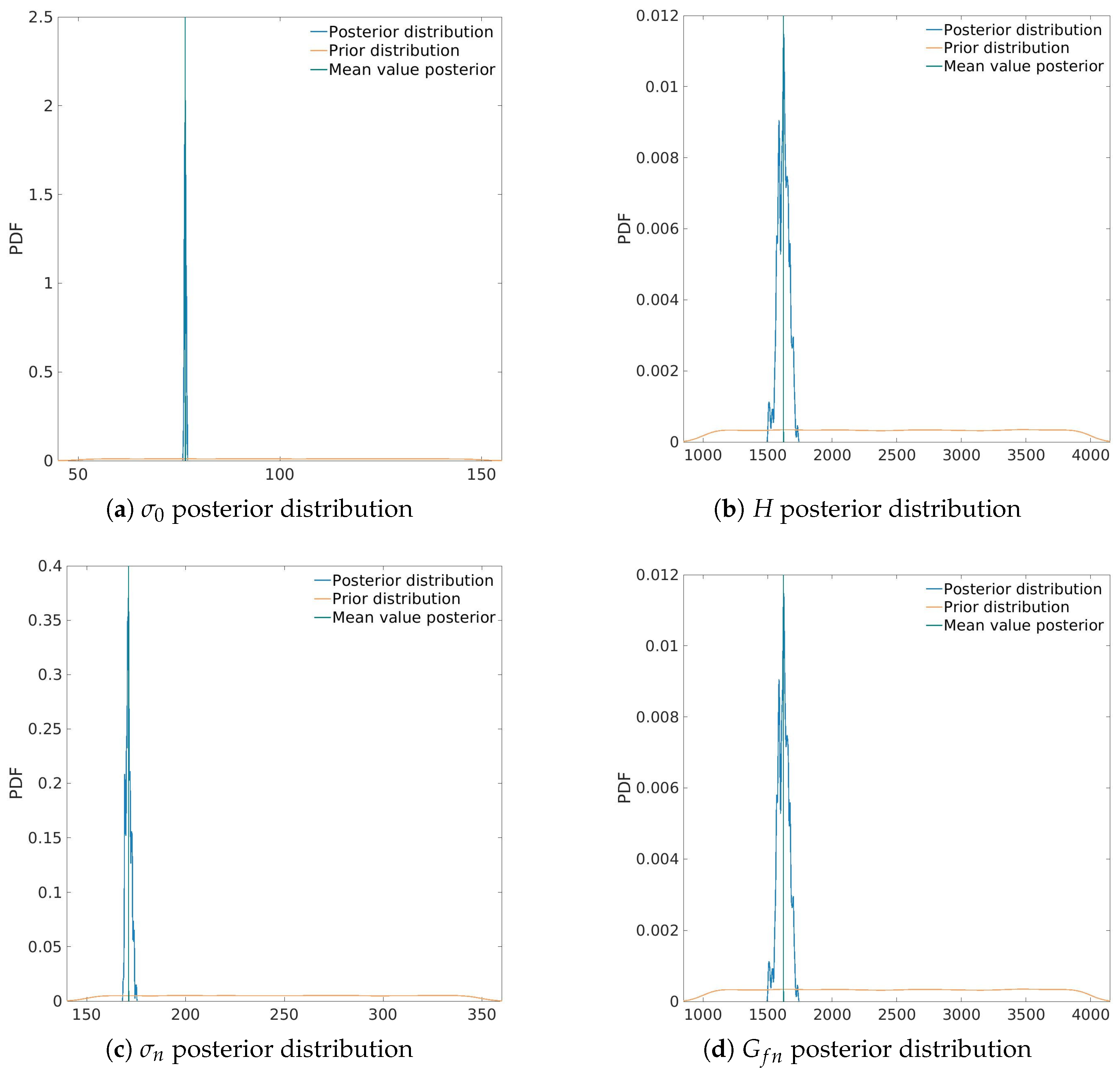
The identification of elastoplastic and fracture parameters was performed using 200 Markov chains and 5000 computational steps, resulting in a total of 1,000,000 evaluations for different parameter combinations. The entire process took less than 10 min to complete. The results are presented in Figure 10.

The posterior distribution of yield strength ${\sigma }_0$ exhibits minimal variation, indicating a high level of certainty, with a maximum posterior value of $76.52{\mathrm{N}/\mathrm{mm}}^2$. Similarly, the hardening modulus H shows only slight variation around its maximum posterior value of $1626.01{\mathrm{N}/\mathrm{mm}}^2$. The posterior distribution of tensile strength ${\sigma }_n$ also demonstrates high certainty, with a well-defined peak at $171.11{\mathrm{N}/\mathrm{mm}}^2$. Finally, while the posterior distribution of tensile fracture energy $G_{fn}$ shows slightly greater uncertainty compared to the other parameters, it still features a strong peak around its maximum posterior value of $258.17\mathrm{N}/\mathrm{mm}$.

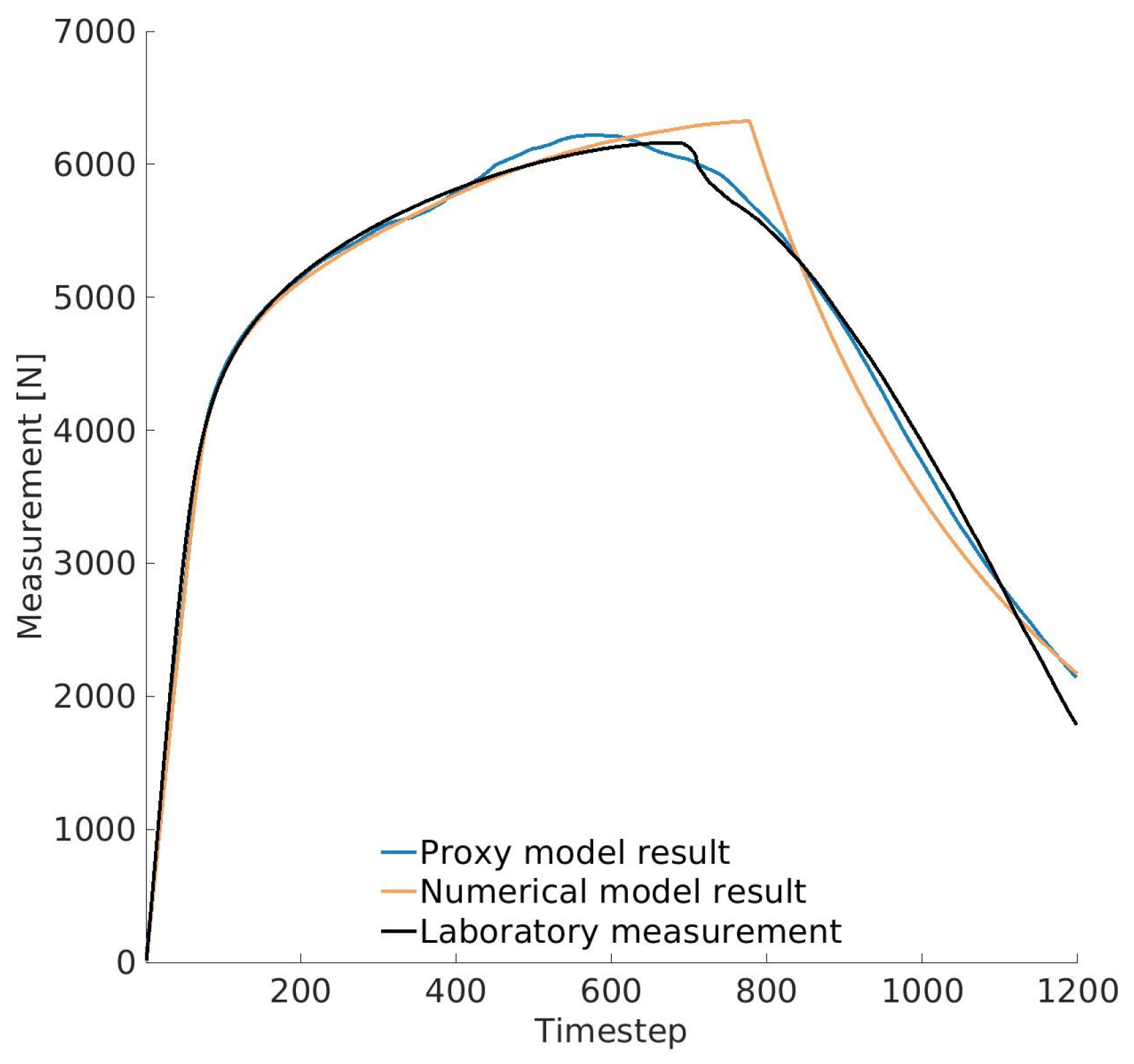
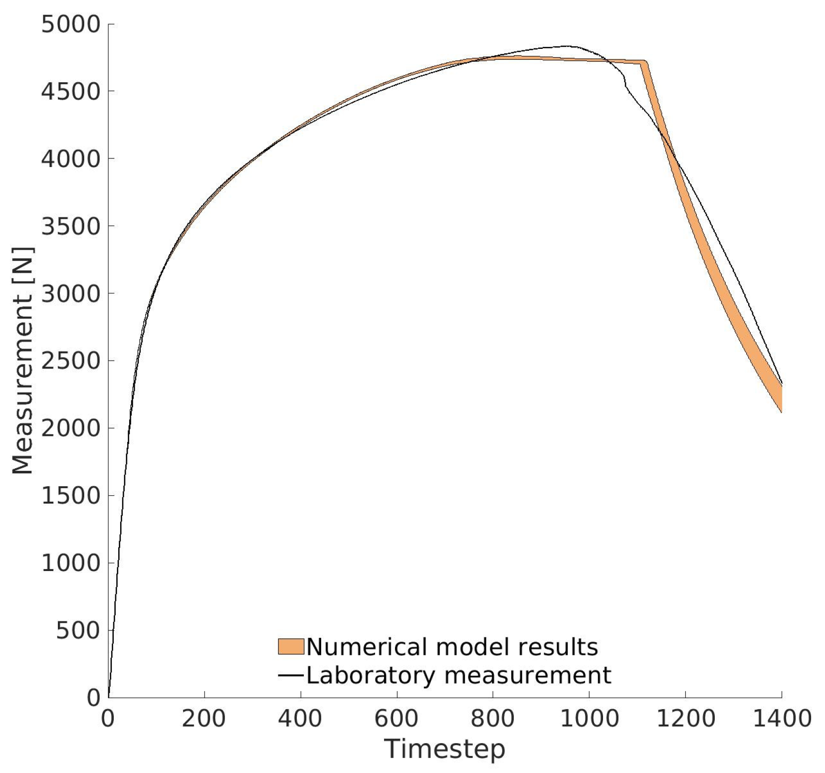
These maximum posterior values were used in both the proxy model and the full numerical model to compare against the experimental data. The comparison is presented in Figure 11. As shown, the proxy model closely follows the lab measurements throughout the test, with only small deviations (with a maximum error of 2%). The numerical model also aligns very well with the experimental results, particularly in the elastic and elastoplastic regions, which confirms the accuracy of the identification process. A slight discrepancy emerges after the onset of fracture, mainly due to differences between the proxy model and the numerical simulation results (see Figure 9). The maximum error between the laboratory measurement and the numerical model is 8.9%. Nevertheless, the accuracy remains good, especially considering the challenges of modeling nonlinear fracture behavior.

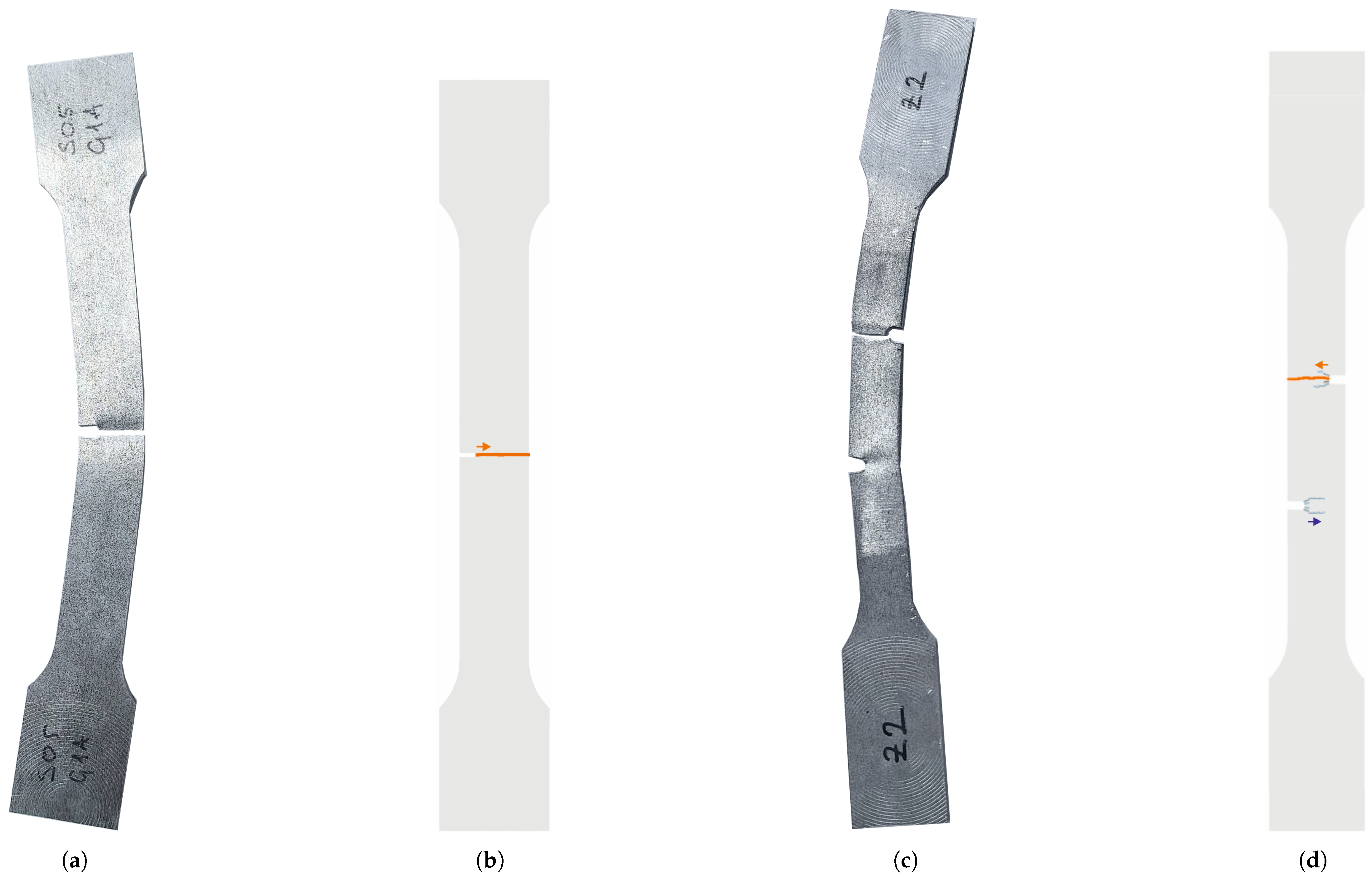
Figure 12 shows a comparison of specimen failure observed in the laboratory tests and in the numerical simulations. For the simulation results, cracks are visualized using a color scale ranging from blue to orange, representing the level of energy dissipation, where blue indicates lower values and orange higher ones. For the single−notched dogbone specimen, both the experimental and numerical results (see Figure 12a,b) confirm the formation of a single dominant crack. This crack initiates at the edge of the notch and propagates toward the end of the specimen perpendicular to the direction of the loading. This confirms that the model accurately captured the failure mechanism.

5.3. Result Verification

The verification of the identified elastic, elastoplastic, and fracture parameters was carried out for two cases by comparing the numerical model results using the MAP estimate of the parameters with two distinct sets of experimental data. The first case involved a comparison of displacements and strain field values on a single−notched dogbone specimen, with data obtained by DIC camera. The second verification used force−displacement data from a double−notched dogbone specimen (see Figure 3c). This approach allowed for validation not only against different types of measurements from the specimen used for identification but also against specimens with different geometries (see

Table 3. Verification process of elastic, elastoplastic, and fracture parameters through comparison of laboratory measurements and numerical model predictions (two verification cases) ¹.

Parameter	Specimen	Measurement
${\sigma }_0,H,{\sigma }_n,G_{fn}$	single−notched	Vertical displacements and strain fields (DIC)
${\sigma }_0,H,{\sigma }_n,G_{fn}$	double−notched	Force–displacement (UTM)

¹ Accuracy of the identified elastic parameter values (E, $\nu$) was confirmed by matching of numerical model results with experimental measurements in the linear elastic region of force−displacement measurements for the single-notch and double-notch specimens.

).

For each verification case, 20 samples were generated from the posterior parameter distributions using QMC sampling. These parameter sets were then used in simulations, and the resulting outputs were compared with experimental data to evaluate the accuracy and robustness of the identification methodology.

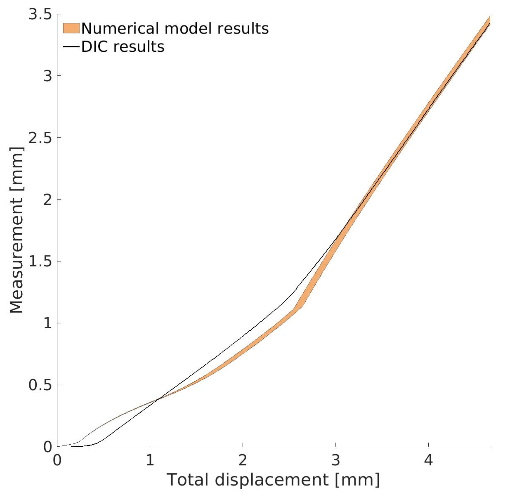
For the first verification case, two points on the specimen were selected: (12 mm, 100 mm) and (12 mm, 120 mm). These points were located on opposite sides of the crack. The vertical displacement difference between these points was extracted from DIC measurements and compared with numerical results, as shown in Figure 13. The results reveal some differences between the numerical and DIC data. The largest discrepancy appears at the beginning of the test, mainly due to the difficulty of DIC systems in capturing very small displacement values accurately. As the test progresses and displacements become larger, the measurements from DIC become more reliable. In the middle of the test, where the measured values are higher, the DIC measurements become more reliable. At this stage, the observed differences are largely attributed to the same sources of error noted in the force−displacement comparison, particularly those arising from the proxy model. The maximum error between the DIC measurements and the numerical model is 11.9%. Toward the end of the test, these differences continue to decrease, resulting in an increasingly close match between the numerical predictions and the DIC data.

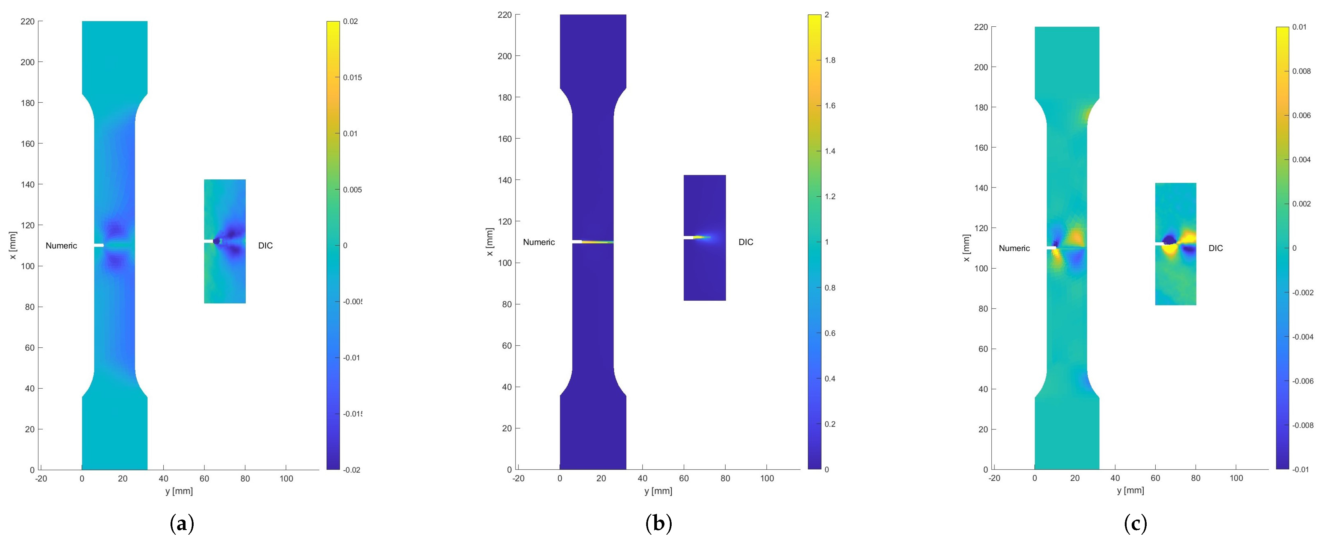
Additionally, a comparison of strain field values was performed for a total displacement of 3.899 mm. The strain components were computed from the displacement gradients using standard DIC post-processing methods. This comparison also showed very good agreement between the two results, both in the shape of the strain fields and the magnitude of the strain values (see Figure 14).

The second verification case was conducted by comparing the force−displacement results from the laboratory with numerical simulation results. This specimen had a different geometry and featured two notches of different sizes, which led to a stress distribution and failure mode different from the ones used for parameter identification. Despite these differences, the comparison shown in Figure 15 demonstrates that the numerical model performed with high accuracy. The elastic and elastoplastic regions were matched almost perfectly. Some discrepancies appeared in the fracture region, similar to what was observed in previous comparisons, with the maximum error reaching 7.8%. These results further support the reliability of the identified parameters, even when the fracture mechanism is different.

A comparison of the failure behavior of the double−notched specimen in both the laboratory and numerical simulation (see Figure 12c,d) shows similar fracture mechanisms. In the laboratory, a macrocrack formed at the upper notch, leading to complete failure, with additional damage observed around the lower notch. The numerical model result follows the same pattern, with a main macrocrack forming from the upper notch, causing total failure. Additionally, due to the wider notches, the formation of several microcracks is visible alongside the macrocrack, though they contribute little to energy dissipation. For the lower notch, a few microcracks are also seen, but they do not significantly dissipate energy, which matches the laboratory results, where only limited damage is visible.

6. Conclusions

This work demonstrates the potential of the Bayesian approach for solving the inverse problem of material parameter identification, specifically applied to the failure behavior of aluminum 6060 alloy specimens.

Within the applied methodology, a numerical model based on the embedded discontinuity method (Q6ED) is used, in which cracks are modeled locally with their own location and orientation. This allows for realistic and mesh-independent fracture results.

To achieve a computationally efficient approach, a generalized polynomial chaos expansion (gPCE) was used as a proxy model. This approach has already proven to be efficient and accurate for simpler fracture cases, while also supporting straightforward sensitivity analysis, which is valuable for both test design and understanding parameter influence. However, gPCE introduces approximation errors that must be carefully controlled across the entire response surface. If not adequately managed, these errors can bias the identification process by overfitting regions with lower proxy error, thereby compromising the accuracy of the identified parameters.

The experimental setup involved tensile testing using a universal testing machine (UTM), with deformation monitored through simple yet effective measurements, including internal UTM sensors (force, crossbar position, and extensometers), LVDT sensors with an additional data acquisition unit, and an optical measurement system. Unlike standard laboratory specimens, the aluminum samples in this study were intentionally designed with notches to induce stress concentrations, which makes them non-standard and typically unsuitable for direct parameter extraction from test data alone.

A key aspect of the Bayesian method is the definition of the error model. In this study, measurement error, modeling error, and proxy model error were assumed to be mutually independent and normally distributed with zero mean. While this assumption is widely used due to its simplicity and analytical convenience, it may not always hold, particularly in the context of nonlinear fracture mechanics. In this work, the assumption of unbiased and uncorrelated measurement errors was considered reasonable due to reliable calibration and stable testing conditions. In contrast, modeling and proxy errors are inherently more complex. They may exhibit correlation, systematic bias, or non-Gaussian behavior, especially near crack initiation. Nevertheless, the error analysis for non-linear data showed that the impact of such limitations was limited. Consequently, the adopted simplifications were deemed justified and did not significantly compromise the validity of the results within the scope of this study.

The Bayesian inversion process successfully provided credible posterior values for key parameters across all behavioral phases: elastic (Young’s modulus E, Poisson’s ratio $\nu$), elastoplastic (yield strength ${\sigma }_0$, hardening modulus H), and fracture parameters (tensile strength ${\sigma }_n$, tensile fracture energy $G_{fn}$). The resulting posterior distributions show limited variability, highlighting the robustness of the Bayesian methodology and the effectiveness of the integrated numerical and experimental framework. However, this level of certainty may not be achieved with different numerical models or experimental conditions. This highlights the importance of applying probabilistic methods for nonlinear and non-standard measurements over deterministic approaches, as they provide a means to quantify uncertainty, which is essential for the reliability and interpretability of the results.

The identified elastic parameters from the rectangular specimen were shown to be applicable to all the subsequently tested specimens. The maximum a posteriori (MAP) values of the elastoplastic and fracture parameters, obtained from the single−notched specimen, were validated through comparisons with independent measurement data and additional results from the double−notched specimen. These comparisons demonstrated a strong agreement with the experimental observations, further confirming the robustness and reliability of the identified parameters within the scope of the conducted tests. However, confirming the broader applicability of the methodology will require further validation through more diverse specimen geometries and multiaxial loading scenarios.

It is important to recognize that the identified parameters are not purely material constants in the classical sense, but are model-dependent. While elastic parameters E and $\nu$, as well as ${\sigma }_0$ and ${\sigma }_n$ may closely reflect intrinsic material properties, hardening modulus H and tensile fracture energy $G_{fn}$ are the parameters calibrated for the specific numerical model applied in the identification process. In this case, isotropic linear hardening and exponential softening were assumed to approximate the complex plastic and failure behavior, respectively. Therefore, while the results support the robustness of the Bayesian approach even with non-standard specimens, the interpretation of the identified parameters should always consider the modeling framework used.

Finally, the demonstrated methodology shows strong potential when complemented with experimental investigations, offering the ability to identify multiple parameters from a single test, even under suboptimal sample geometry. As a part of future work, we aim to refine the error modeling by explicitly accounting for correlations in proxy and modeling errors. Additionally, broader experimental validation will be necessary to confirm the generalizability of the approach. With further development and testing, this framework could be extended to a wide range of engineering applications, particularly where standard specimens are unavailable or full-scale testing is impractical.