Article

Research on Laser Radar Inspection Station Planning of Vehicle Body-In-White (BIW) with Complex Constraints

School of Mechatronic Engineering, Xi’an Technological University, Xi’an 710021, China
*
Author to whom correspondence should be addressed.
Appl. Sci. 2025, 15(11), 6181; https://doi.org/10.3390/app15116181
Submission received: 27 April 2025 / Revised: 19 May 2025 / Accepted: 28 May 2025 / Published: 30 May 2025

Abstract

:
This study develops an applied optimization method to address practical challenges in Laser Radar station planning for automotive Body-In-White (BIW) manufacturing inspection. Focusing on the spatially constrained industrial environments and complex measurement specifications, the work reformulates Laser Radar inspection planning as a multi-constrained optimization problem challenge. Firstly, a parametric geometric modeling approach is developed to define measurement spaces for individual features, accompanied by an innovative maximal complete subgraph mining algorithm to intelligently identify shared feasible measurement regions among multiple features. Secondly, kinematic equations are formulated using Denavit–Hartenberg (D-H) parameters, while a hierarchical bounding volume collision detection mechanism is integrated to establish a comprehensive constraint. Therefore, unified optimization method synergizing measurement coverage, robotic manipulator reachability, and operational safety requirements are proposed. Through experimental validations utilizing BIW (BIW) component inspection, the research has demonstrated its industrial applicability and has achieved a 92% measurement coverage with robot trajectories free of collisions. Compared with traditional manual planning methods, the proposed approach reduces the number of required inspection stations by 35% and improves the computational efficiency to meet industrial real-time deployment requirements. Experimental validation demonstrates the method’s effectiveness in measurement accuracy, operational safety, and equipment utilization for advanced manufacturing quality control systems.

1. Introduction

As the core skeletal structure of automotive manufacturing, the BIW serves as both the structural foundation and assembly platform for all vehicular components. The dimensional accuracy of the BIW establishes the fundamental prerequisite for superior vehicle quality [1]. The practical issues and requirements in the measurement process of the BIW include the following [2,3]: (1) The high production tempo in automotive manufacturing requires highly efficient measurement. (2) Numerous inspection features need to be measured, which are extensively distributed spatially. (3) The limited accessibility of complex curved surfaces and complex measurement environments cause measurement interference. (4) The measurement tasks for automotive manufacturing exhibit significant variability and dynamic characteristics. With the advancement of intelligent manufacturing capabilities, the automotive industry faces new challenges in the measurement methods, efficiency, and flexibility for evaluating product quality characteristics during BIW production processes.
Various metrology techniques, such as machine vision, coordinate measuring machines (CMMs), laser scanning systems, and digital twins, can be used to inspect the BIW [4,5,6,7,8,9,10]. A touch-trigger probe CMM and a laser scanner CMM were compared as offline measurement systems against a Laser Radar as an inline solution [2]. Armagan and Emre made the assessment of the measurement capability for the Hexagon Leica laser scanning system and evaluated the possibility of replacement with an actual CMM in BIW measurements [3]. CMMs are commonly used in online measurement processes in the automotive industry at present. But limited by the measurement efficiency, the sampling rate cannot be promoted in quality monitoring. The Laser Radar provides automated, non-contact measurement capability for medium- to large-volume applications with an accuracy comparable to that of the CMM system. Laser Radar is common in aerospace, wind power generation, and so on. Sanderson (2020) [11] issued an accurate measurement technique by using coherent Laser Radar. The advantages of Laser Radar for large-scale measurement were analyzed. Jeremy (2016) [12] described the measurement error affected from the inspection range, azimuth, and elevation. From the analysis, it is observed that coherent Laser Radar is suitable for complex large-scale workpieces. Wang (2013) [13] focused on investigating the errors which arise during the measurement process and the uncertainty calculations for the measurements. The distribution of tooling balls could be determined based on the proposed error model. As demonstrated in prior studies, Laser Radar is suited to automating repetitive inspection tasks and provides greater flexibility for the BIW’s online inspection in the automotive industry.
Limited by the characteristics of laser inspection and feature distribution, the Laser Radar needs to be placed at a series of positions, referred to as laser stations, to cover all the features to be measured. Therefore, the industrial robot is introduced to hold the Laser Radar to reach the desired stations. To provide guidance for controlling the robot, station planning is required before robot motion programming. Liu (2008) [14] proposed a systematic algorithm for generating optimal inspection planning for free-form surface inspection. It changed “SMR moving and laser beam tracking” to “3laser beam moving and SMR tracking”. Larsson (2008) [15] concentrated on automatic path planning for laser scanning with an industrial robot. Some open type parts were used to verify the feasibility of the proposed method. Mahmud (2011) [16] proposed path planning under guaranteeing the measurement accuracy during the scanning with regard to the geometrical product specifications. Wang (2014) [17] proposed scanning path planning and process parameters based on the projection decomposition method. Zhang (2016) [18] presented a rapid laser scan planning method that overcomes the computational complexity of planning laser scans based on diverse data quality requirements in the field. The planning goal is to minimize the data collection time while ensuring that the data quality requirements of all objects are satisfied. Zhao (2016) [19] combined a touch-trigger probe and a laser scanner to fulfil the accuracy and complexity of measurement requirements. Lee (2000) [20] proposed an algorithm to plan how to place the scanner to satisfy the view angle, view depth, and interference requirements. Du (2016) [21] offered an error-ellipsoid-based uncertainty model for Laser Radar measurement. The abovementioned planning research focused on the measurement accuracy or collection time. Because the parts under inspection typically have flat surfaces, the occlusion, reachability, and interference are not prominent problems in path planning. Coherent Laser Radar provides a robust and highly accurate form of measurement for the BIW. However, the features to be measured of large-scale spatial distribution and complex inspection constraints become a challenge in the BIW inspection implementation of Laser Radar.
In BIW inspection using Laser Radar systems, the laser and the feature are constrained within certain angle and distance ranges to ensure the inspection accuracy. Moreover, the laser must not be obstructed before reaching the feature. For safety, the Laser Radar must not collide with the ground, walls, or BIW. Additionally, the Laser Radar must not be positioned in a location that the robot cannot reach. When these complex constraints are incorporated into the station optimization model, the measurability of the planning result can be ensured. This paper focuses on the abovementioned constraint models. This paper is organized as follows: In Section 2, the station planning of BIW inspection is described in detail. In Section 3, the measurement constraints for BIW inspection are established. Section 4 provides a case study to verify the proposed methods. Finally, conclusions are presented in Section 5.

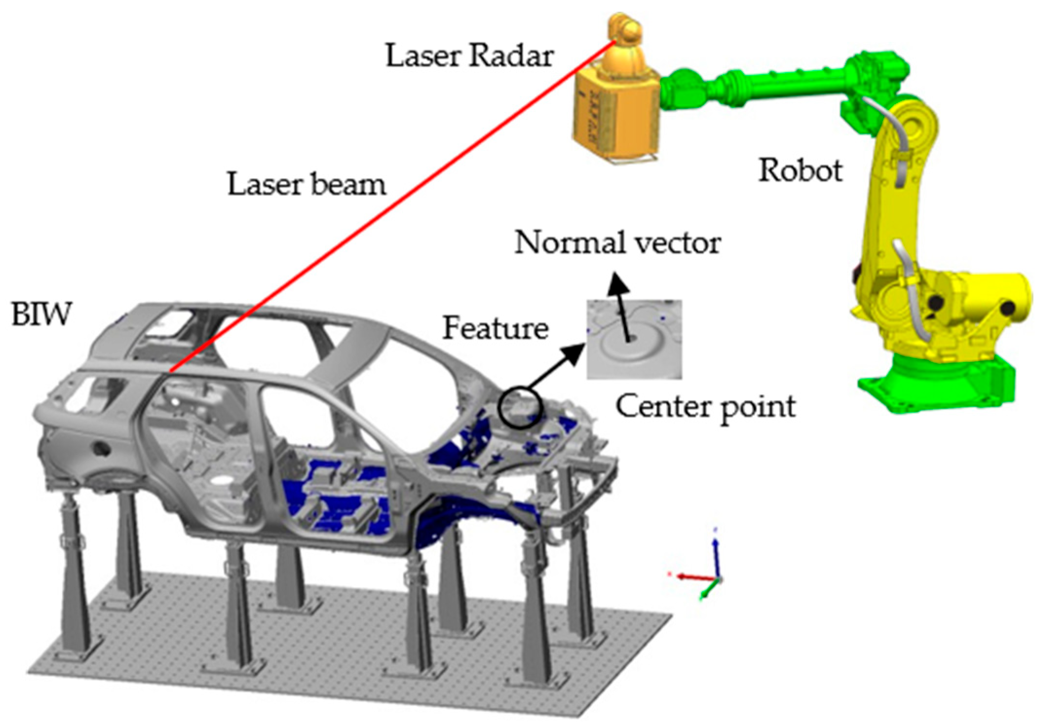
2. Engineering Problem for Laser Radar Station Planning of BIW Inspection

The dimensional accuracy elements of the BIW primarily consist of three key features: points, holes, and slots. These measurement features are predefined in body dimension engineering design, with their fundamental attributes including positional coordinates and directional vector information (Figure 1). Due to the complex surface geometry of the measured BIW, the numerous measurement features, and the varying distances and irregular distribution between these features, a single measurement station cannot achieve full-coverage measurement. Multiple measurement stations are therefore required to comprehensively measure the BIW. Since measurement field errors may arise during the station transfer process of the Laser Radar, the station layout should be optimized to minimize the number of stations within a fixed measurement space. Furthermore, under constrained measurement resources, the measurement efficiency could be improved with fewer stations through the induction of the instrument repositioning time. Therefore, the goal of the Laser Radar station planning is to determine the minimum measurement stations required to achieve the full-coverage dimensional deviation measurement of the BIW.
The ranging measurement between the Laser Radar and target features is accomplished through time-of-flight detection, where the receiver module precisely captures the phase-shifted optical signals retroreflected from measured surfaces. By combining the calibrated beam emission vector (azimuth (θ) and elevation (φ)) with the radar’s geodetic coordinates [X, Y, Z] in the global frame, the spatial position of each feature is analytically derived through trigonometric transformation, achieving micron-level coordinate determination accuracy. Prior to the station planning of Laser Radar inspection, key definitions are established, as illustrated in Figure 2.
The inspection coordinate system refers to the global coordinate system in the workspace. The features to be measured and Laser Radar stations are defined in this coordinate system. It can be denoted as (OM, XM,YM, ZM).
A feature refers to a specific point or area to be inspected on the BIW. The center point of the i-th feature is denoted as Fi, and its normal vector is denoted as Ni.
The inspection distance is the distance from the radar to the feature Fi. It is denoted as Di for Fi.
The inspection angle is the angle between the laser beam and normal vector of the feature. It is denoted as θi for Fi.
The inspection area defines the reachable region of the radar’s laser beam. The pitch angle of the laser beam is ±45°, and the rotation angle is 0°~360°.
A station is the position and posture where the Laser Radar is placed in the workspace. It is denoted as S k = p k , v k . pk is the position of the radar station, and vk is the vector of the station posture.
To guarantee the inspection accuracy, the inspection distance must be within a specific range. Similarly, the inspection angle should be maintained within a defined range. The optimal placement of the Laser Radar is within a region that meets the accuracy requirements for the inspection of multiple features.
The constraints in this study are divided into three categories: position constraints, interference constraints, and spatial constraints. The position constraints include the inspection angle and distance. The purpose of the interference constraints checking is to prevent laser beam interference. The spatial constraints encompass the space interference and robot reachability requirements.

3. Measurement Constraints for BIW Inspection

3.1. Position Constraints of Station Planning

In the context of radar station configuration, the feasible region for a feature to be measured is determined by both the inspection distance and inspection angle. Li and li are the maximum and minimum allowed inspection distances. αi is the maximum allowed inspection angle of the feature to be measured. The feasible region corresponding to Fi is denoted as Ai (Figure 3a). The shared feasible region among multiple features is shown in Figure 3b.
In the context of inspection operations, minimizing the number of Laser Radar stations is advantageous, as station switching is time-consuming. A Laser Radar station shared among multiple features can reduce the overall number of stations needed.
However, conducting measurability checks between each station and feature significantly increases the planning time. To address this, reducing the feasible region of the planning area can eliminate unnecessary checks. Identifying shared feasible regions efficiently is crucial. An attributed adjacent graph (AAG) is employed to record intersection relationships. However, with a large number of features, the AAG becomes too intricate for intersection searches. Therefore, a clustering algorithm is applied to classify features before constructing the AAG, improving the process’s efficiency and manageability.
The clustering steps for the features to be measured are as follows (Figure 4):
  • A local coordinate system is assigned for each measuring feature. The origin is the center point (Fi). The Z axis is along the normal vector pointing outward from the material surface at Fi;
  • The K-means++ algorithm is used to cluster feasible regions. The number of features in each cluster is constrained to a manageable size;
  • In the local coordinate system of the feature, a point denoted as C i is defined:
C i = 0,0 , 0.618 L i , 1 T
4.
The transformation matrix from the local coordinate to the inspection coordinate is denoted as T. The point ( C i ) in the inspection coordinate system is denoted as C i :
C i = T C i
5.
The distortion function in clustering is J, and μc is the centroid of a cluster:
J = i = 1 m C i μ c 2
6.
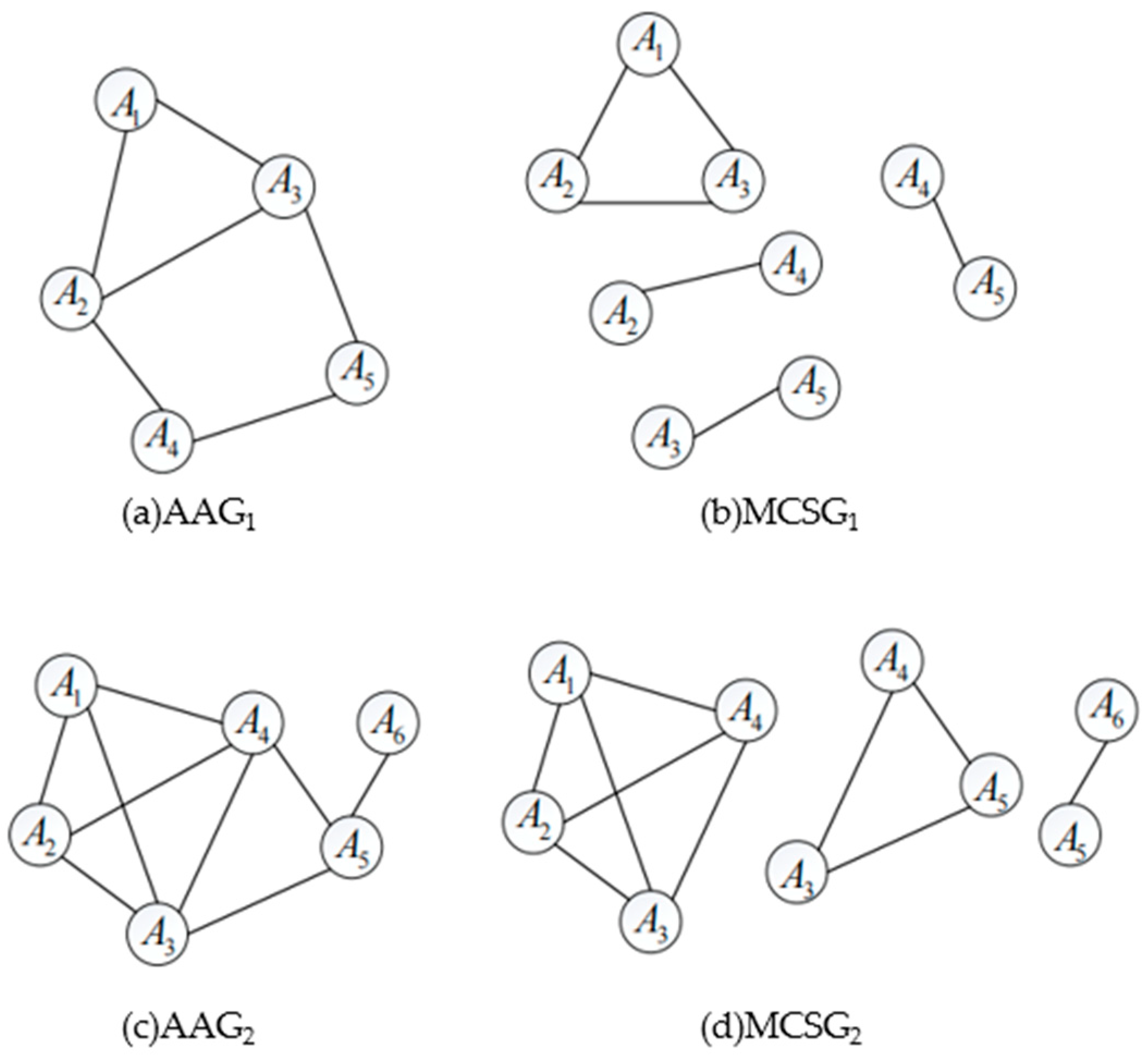
The clustering result is denoted as Gi. In each Gi, the intersections of the feasible regions are checked to construct the AAGi.
It is difficult to express the shared area of feasible regions precisely. Therefore, the feasible region should be simplified first. The inspection distance is l i D i L i . The inspection angle is 0 θ i α i . The feasible region (Ai) could be simplified into a group of spherical regions (Figure 5). The approximation steps for feasible regions are as follows:
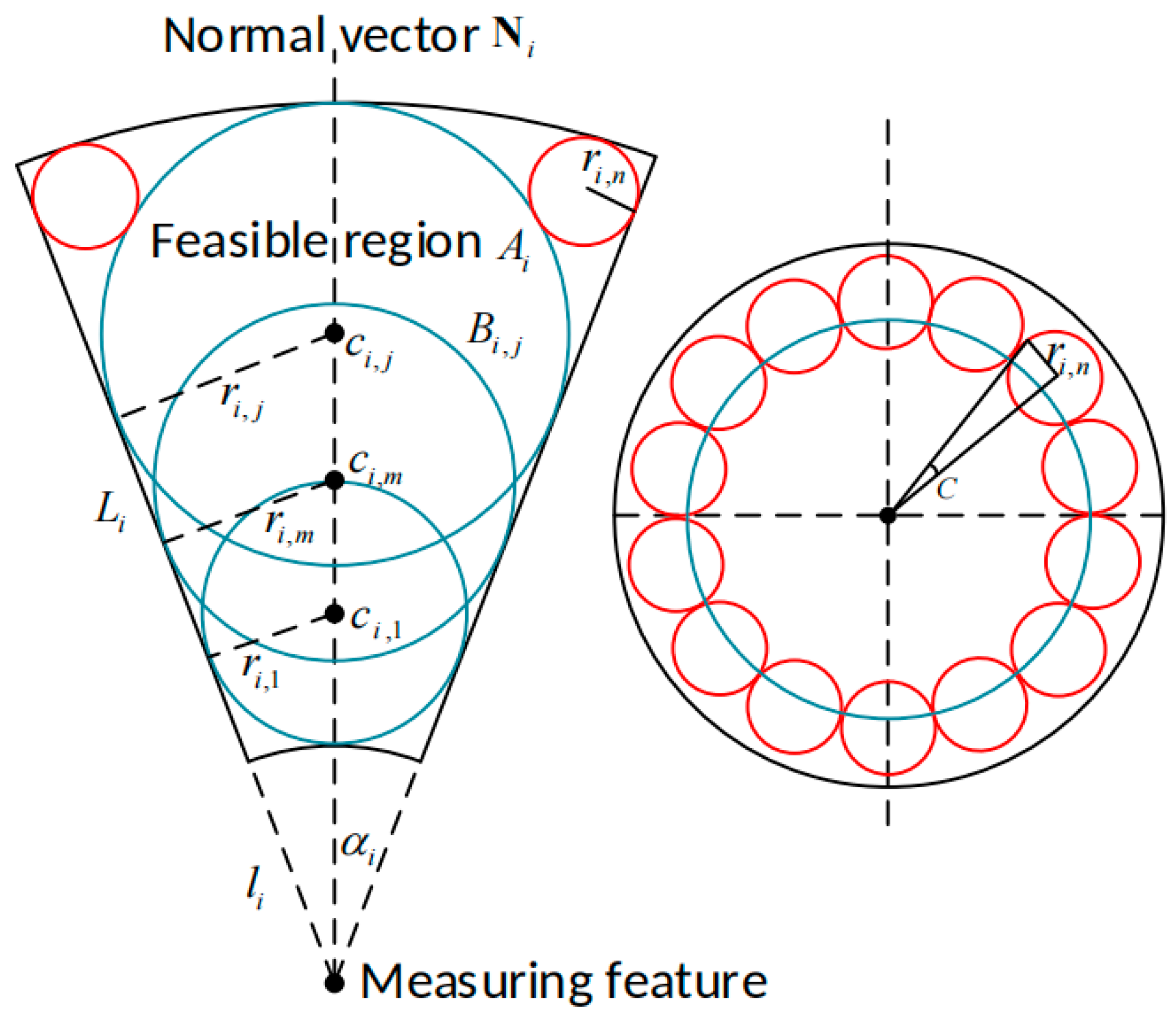
  • The feasible region is simplified into a group of basic spherical regions and supplementary spherical regions which are denoted as follows:
    B i , j = ( c i . j , r i , j )
    where c i , j   a n d   r i , j   d e n o t e the sphere’s center coordinates and radius, respectively. The number of basic spherical regions is m:
For the first spherical region, c i , 1   a n d   r i , 1   are expressed as follows:
c i , 1 = 0   0   l i 1 s i n α i 1
r i , 1 = l i sin α i 1 sin α i
For the last spherical region, c i , m   a n d   r i , m   are expressed as follows:
c i , m = 0   0   L i 1 + s i n α i 1
r i , m = L i s i n α i 1 + s i n α i
For the n-th middle spherical regions, n = 1,2 , m 2 , and c i , n   a n d   r i , n   are expressed as follows:
c i , n = n c i , j + ( m n ) c i , 1 m
r i , n = ( n m ( L i l i r i , j r i , 1 ) + l i + r i , 1 ) sin α
2.
In the supplementary spherical regions, c i , n and ri,n yield the following equations:
( r i , j + r i , n ) 2 = ( L i r i , j ) 2 + ( L i r i , n ) 2 ( L i r i , j ) ( L i r i , n ) cos A A = α i arcsin r i , n L i r i , n
c i , n = cos A 0 sin A 0 0 1 0 0 sin A 0 cos A 0 0 0 0 1 cos C sin C 0 0 sin C cos C 0 0 0 0 1 0 0 0 0 1 0 0 ( L i r i , n ) cos A 1
C = n 2 a r c t g ( r i , n ( L i r i , n ) sin α i ) , n = 0,1 , , 2 π / C
The intersection of the feasible regions are determined by the intersection of the spherical regions. The shared-feasible-region searching steps are as follows:
  • Two feasible regions (Ai and Am) are discretized into two groups of spherical regions. They are sorted into the sets below, corresponding to Ai and Am:
B i , j = c i , j , r i , j
B m , n = c m , n , r m , n
2.
The Bi,j and Bm,n are traversed, and each spherical region in set Bi,j is combined with every spherical region in Bm,n. The combination group is denoted as B i , j , B m , n ;
3.
If any combination in B i , j , B m , n yields to Equation (16), the feasible region (Ai) intersects with Am. If not, B i , j , B m , n yields to Equation (16), and the feasible region (Ai) does not intersect with Am:
c m , n c i , j r m , n + r i , j
4.
If two feasible regions (Ai and Am) are intersected, an edge, denoted as E (Ai, Am), is added between corresponding vertexes, representing feasible regions, in the attributed adjacency graph;
5.
The AAGi is built up when each feasible region has been checked with the others in cluster Gi;
6.
In the AAGi, the maximal complete subgraphs are identified, which are denoted as MCSGi,j. The features to be measured in MCSGi,j have shared feasible regions;
In Figure 6a,c, an AAG is constructed based on intersection checking. The maximal complete subgraphs are identified and presented in Figure 6b,d.
The station of the Laser Radar is in the shared feasible region in the MCSGi,j. The feasible region (Ai) is scattered into B i , j , as shown in Equation (16).
The distance between the station (Sk) and Bi,j is   d i , j , k and is expressed as follows:
d i , j , k = p k c i , j
If d i , j , k r i , j , it means that the station (Sk) is in the feasible region (Ai). So, the position constraint is as follows:
d i , j , k r i , j 0
where i is the number of feasible regions (Ai) in the MCSGi,j, j is the number of discrete spherical regions belonging to Ai, and k is the number of the station.
The position constraint is established through the following steps:
  • Clustering Features: the features to be measured are clustered into Gi using the clustering algorithm described previously;
  • Approximating Feasible Regions: the feasible region (Ai) of feature Fi is discretized into a set of spherical regions (Bi,j) through feasible region approximation;
  • Constructing AAG Subgraphs: The intersection between the feasible regions (Ai) within Gi is checked to construct the attributed adjacency graph (AAGi). The maximal complete subgraphs (MCSGi,j) in the AAGi represent the shared feasible regions;
  • Defining Position Constraints: the station’s position constraint is determined by evaluating the distance between the station and the approximated spherical regions (Bi,j).

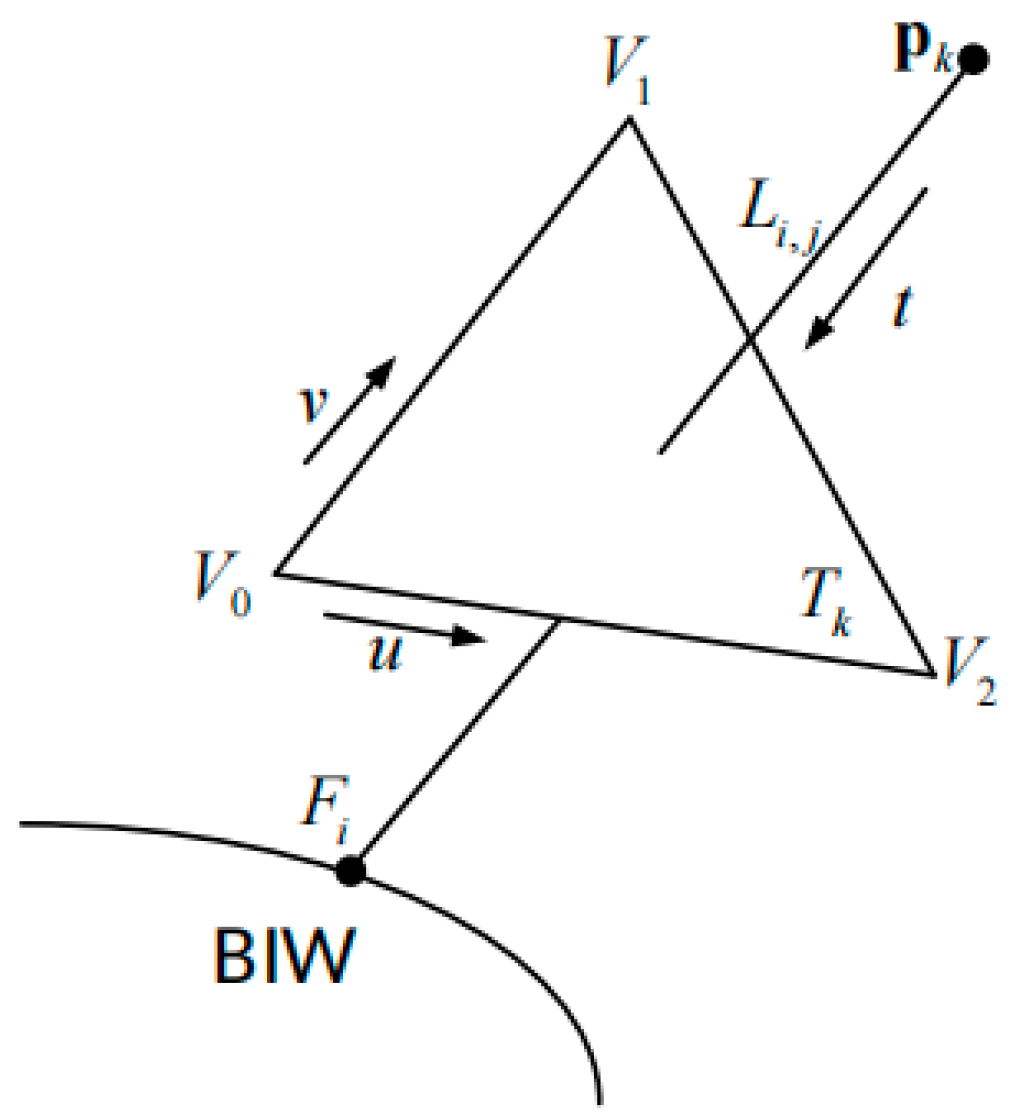
3.2. Interference Constraints of Station Planning

An additional critical constraint in station planning is ensuring the laser’s unobstructed path to the feature to be measured. For interference verification, the BIW model, exported in STL format and represented by a multitude of triangles, is utilized. Interference checking is thus replaced by collision detection between the laser and these triangles.
The laser beam is from station Sj to Fi. It can be represented as follows:
L i , j = p j + D t
where
D = F i p j F i p j
The triangle Tk is represented as follows:
T k = ( 1 u v ) V 0 + u V 1 + u V 2
V0, V1, and V2 are the vertex of triangle Tk. If Li,j intersects with Tk, the system yields solutions in u, v, and t for the following equations (Figure 7):
D V 1 V 0 V 2 V 0 t u v = p j V 0
t u v = 1 D × E 2 E 1 T × E 1 E 2 D × E 2 T T × E 1 D
E 1 = V 1 V 0 E 2 = V 2 V 0 , T = p j V 0
The interference constraint is built up as follows:
t F i p j , u < 0 v < 0 u + v > 1
To improve the checking speed, the bounding box and multi-way tree technologies are used to reduce the judgement times.

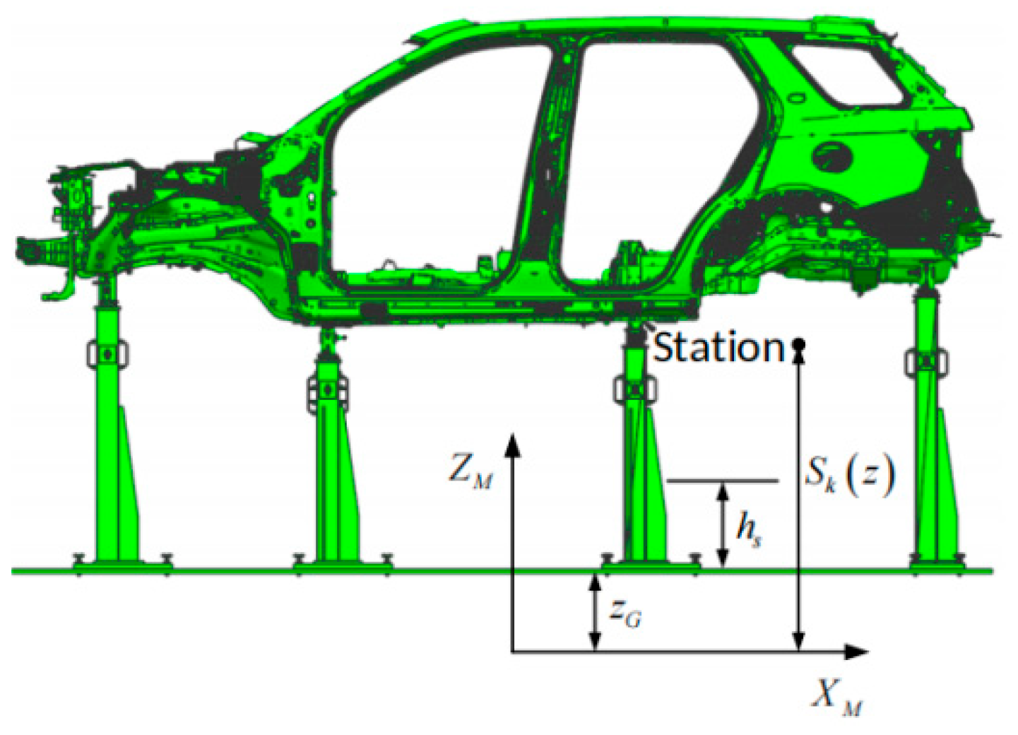
3.3. Spatial Constraints for BIW Inspection
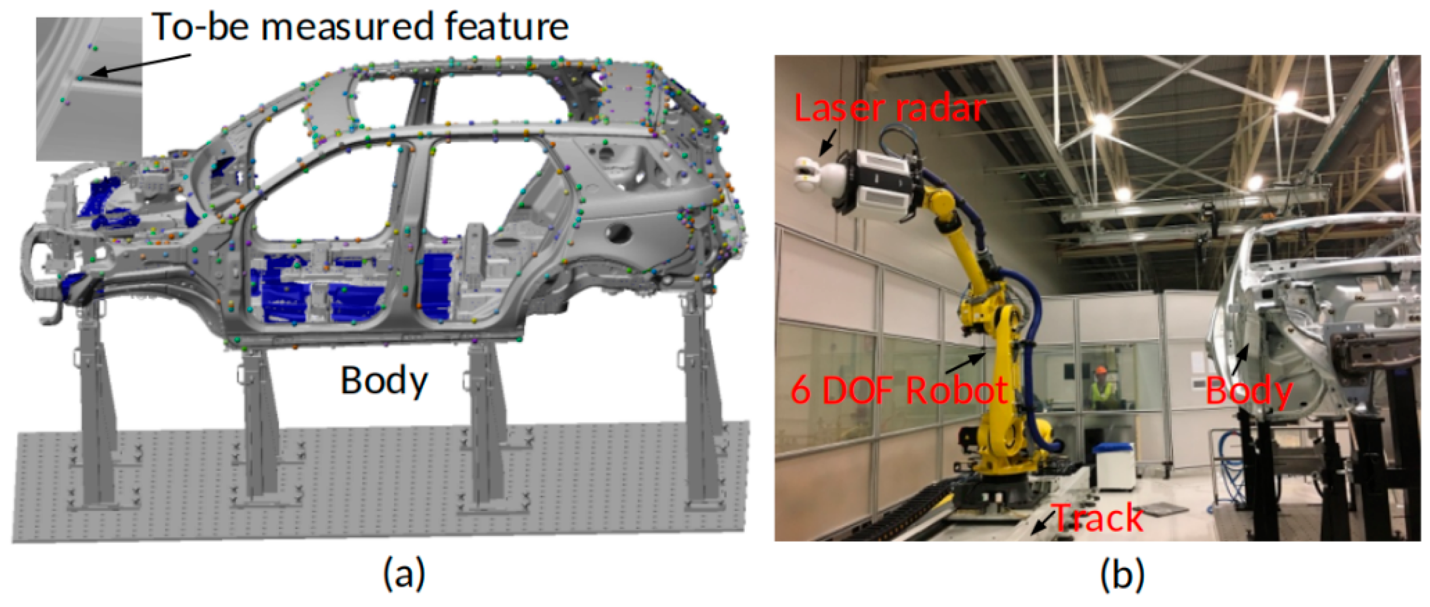
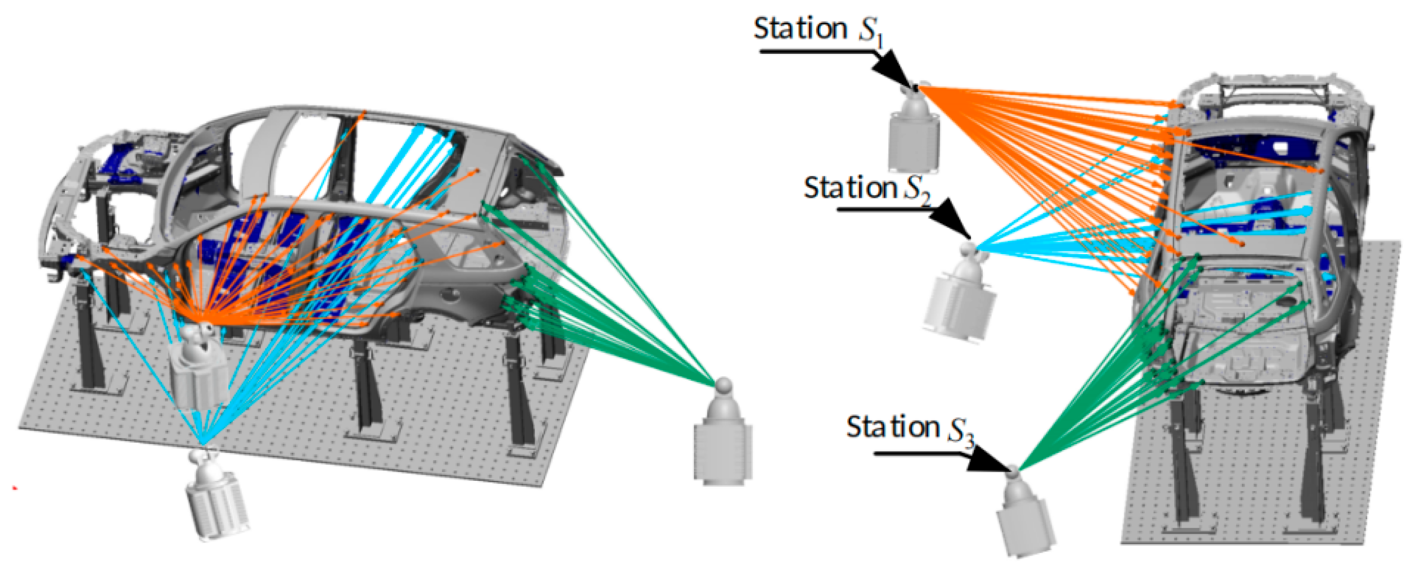
The Laser Radar must avoid collisions with both the ground and the BIW during station operation. Within the inspection coordinate system, the ground is defined as a plane with a constant Z-coordinate of zG. Considering the physical dimensions of the Laser Radar, a safe distance (hs) from the ground is necessary (Figure 8). Consequently, the collision-avoidance constraint is formulated as follows:
J 0 = z G + h s S k ( z ) 0
To avoid the Laser Radar colliding with the BIW, four orthogonal datum walls are assumed around the BIW. The station needs to be outside of the virtual walls (Figure 9). Within the inspection coordinate system, four walls are constructed as modular fixturing assemblies comprising the following:
    x ,   W / 2 ,   z ,   1   w 1 x , W / 2 ,   z ,   1 w 2 L / 2 ,   y ,   z ,   1   w 3   L / 2 ,   y ,   z ,   1 w 4
So, the constraints are as follows:
J 1 = ( W / 2 S k ( y ) 0 ( S k ( y ) + W / 2 0 )
J 2 = ( S k ( x ) L / 2 0 ( S k ( x ) + L / 2 0 )
The collision constraints are combined as follows:
J = J 0 | ( J 1 J 2 )
The Laser Radar is mounted on a robot, so the Laser Radar station must be positioned within the robot’s reachable area. To ensure that the station remains within this accessible region, the robot’s workspace boundary must be defined.
A 6-DOF industrial robot is chosen for radar mounting (Figure 10a). It can be simplified to a linkage model (Figure 10b), with local coordinate systems defined at corresponding joints. Parameters about industrial robot’s arms are listed in Table 1.
The transformation matrix between adjacent coordinates is as follows:
T i i 1 = c β i s β i c α i s β i s α i α i c β i s β i c β i c α i c β i s α i α i s β i 0 s α i c α i d i 0 0 0 1 , i = 1 , 2 , , 6
In the matrix, s means the sine function and c means the cosine function. The subscript is the angle between the axes of adjacent joints. For example, sβi means sin(βi) and cαi means cos(αi).
The robot’s coordinate does not coincide with the inspection coordinate. The transformation matrix between them is as follows:
T o M = 0 1 0 x 0 1 0 0 y 0 0 0 1 z 0 0 0 0 1
The optimized radar’s posture on the station is ensured by the last wrist of the robot. Point is the center of P robot’s last wrist (Figure 10a). Therefore, for any planned station, it cannot be outside of the P region that it can reach.
In the inspection coordinate system, the reachable region of P is denoted as ΩF:
Ω F = x F y F z F 1 = T O M T 1 O T 2 1 T 3 2 P ,   P = 0 0 d 4 1
A station is planned that is S K = ( p k , v k ) , p k = ( x k , y k , z k ) , v k = ( v 1 , v 2 , v 3 ) . The coordinate transformation matrices between the world frame and radar station coordinate system are given below:
T 4 5 = c v 4 0 s v 4 0 s v 4 0 c v 4 0 0 1 0 0 0 0 0 1
T 5 6 = c v 5 s v 5 0 0 s v 5 c v 5 0 0 0 0 1 L 1 0 0 0 1
T M 6 = 1 0 0 x k v 1 L 2 0 0 1 y k v 2 L 2 0 1 0 z k v 3 L 2 0 0 0 1
If the Sk is identified, the feasible area of P is denoted as ΩF:
Ω F = x B y B z B 1 = T 6 M T 5 6 T 4 5 P ,   P = 0 0 0 1
If ΩF intersects with ΩF, the planned station accessible to the robot is operationally feasible.
A group of planes (Ψi), parallel to XMOYM, is defined by a series of different Z coordinate values in the workspace. If a plane intersects with both ΩB and ΩF, the intersection curves are circles, which are denoted as ( P i B , r i B ) and ( P i F , r i F ) , respectively. Then, the robot constraint is that there is a plane (Ψi) which can satisfy the following:
P i B P i F r i B + r i F

4. Experiments

In the experimental verification protocol, a production-representative automotive BIW closer L550 was strategically selected and instrumented with 979 parametrized measurement features. Each feature contains unique alphanumeric identifiers (e.g., L22A781CRE), spatial coordinates, surface-normal vector orientations, and dimensional specifications, including hole diameters and stud protrusion heights (Figure 11a).
The metrological setup incorporated a Nikon Metrology MV331 Laser Radar system mounted on a Fanuc R-2000i robotic arm, where the hybrid metrological system is designed through controller-based inspection station optimization implementation (Figure 11b). This configuration enabled the automated scanning of the parametrized features while maintaining alignment with the predefined measurement protocols.
Traditional approaches employ preconfigured measurement stations around the BIW periphery, where the measurable features are determined based on distance and angular constraints. However, this paradigm suffers from excessive unmeasurable features (113 instances in our validation) and fails to yield satisfactory solutions due to the resource competition among the measurement stations during constraint verification. In experimental trials with 70 predefined seed stations, only 35 proved practically viable. By contrast, our methodology achieves a measurable coverage of 932 features (primarily concentrated on the vehicle underbody with the measurement vectors oriented groundward) using merely 22 optimally configured stations, resolving feature accessibility conflicts through systematic constraint coordination.
The measurement feature data are listed in Table 2.
The attributed adjacent graph in terms of each cluster is determined by intersection checking. Some features to be measured with the shared feasible regions in cluster 1 are listed in Table 3.
In this case, Z G = 900 , h s = 300 . According to Equation (22), the ground constraint is as follows:
S k ( z ) z G + h s = 600
According to Equations (24)–(26), to keep the Laser Radar from colliding with the BIM, the constraints are as follows:
J 1 = ( S k ( y ) 1900 ( S k ( y ) 1900 ) J 2 = ( S k ( x ) 2000 ( S k ( x ) 2000 )
The robot’s reachable area is decided by its location while selected. The data on the special robot are shown in Table 4, and the feasible region of stations is shown in Figure 12 when only the reachable area constraint of the wrist is considered.
Finally, the optimized measurement stations were positioned with the coordinates and scanning directions corresponding to the feature orientations, which are listed in Table 5. Part of the stations are displayed in Figure 13.

5. Conclusions

An applied optimization method is proposed to systematically formulate Laser Radar station planning for automotive BIW metrological inspection into a multi-constrained optimization problem. In contrast to conventional methods that heuristically pre-assign initial stations across the workspace, this approach establishes the global feasible region through geometric feature clustering and spatial intersection analysis, subsequently constructing an attributed adjacency graph to identify the maximum mutual accessibility domains. While traditional inspection configuration relies on fixed-position Laser Radar, the proposed hybrid system implements a robotic manipulator mounted Laser Radar. The kinematic reachability envelope of the robotic system generates piecewise-continuous accessibility boundaries, which are encoded as nonlinear inequality constraints within the optimization formulation.
Furthermore, multiple physical constraints, including optical interference and collision constraints, derived from inspection characteristics and workspace limitations are incorporated into the station optimization model. This comprehensive approach determines the feasible placement region for the Laser Radar during the optimization phase. Experimental verification demonstrates the effectiveness of the proposed methods. Future extensions will investigate uncertainty-aware station planning incorporating metrological error propagation models with accuracy-influencing factors such as the inspection distance and inspection angle.

Author Contributions

Conceptualization, L.L. and X.G.; Methodology, L.L.; Software, J.M.; Investigation, X.G.; Data curation, S.W. and J.M.; Writing—original draft, L.L.; Visualization, S.W.; Funding acquisition, X.G. All authors have read and agreed to the published version of the manuscript.

Funding

This research was funded by The Project Supported by the Natural Science Basic Research Plan in Shaanxi Province of China, grant number 2023-YBGY-123.

Institutional Review Board Statement

Not applicable.

Informed Consent Statement

Not applicable.

Data Availability Statement

The data presented in this study are available upon request from the corresponding author.

Conflicts of Interest

The authors declare no conflicts of interest.

References

  1. Fu, Y.K.; Yang, G.H.; Ma, H.J.; Chen, H.; Zhu, B. Statistical Diagnosis for Quality-Related Faults in BIW Assembly Process. IEEE Trans. Ind. Electron. 2023, 70, 898–906. [Google Scholar] [CrossRef]
  2. Kiraci, E.; Palit, A.; Donnelly, M.; Attridge, A.; Williams, M.A. Comparison of in-line and off-line measurement systems using a calibrated industry representative artefact for automotive dimensional inspection. Measurement 2020, 163, 108027. [Google Scholar] [CrossRef]
  3. Armagan, A.; Emre, B. Comparison of off-line laser scanning measurement capability with coordinate measuring machines. Measurement 2021, 168, 108228. [Google Scholar]
  4. Xi, Z.; Zhou, J.; Yang, B.; Zhang, Y.; Zhang, Z.; Li, D. An intelligent inspection method for BIW weld quality based on vibration excitation response signals. Measurement 2024, 229, 114482. [Google Scholar] [CrossRef]
  5. Li, H.; Li, B.; Liu, G.; Wen, X.; Wang, H.; Wang, X.; Zhang, S.; Zhai, Z.; Yang, W. A detection and configuration method for welding completeness in the automotive BIW panel based on digital twin. Sci. Rep. 2022, 12, 7929. [Google Scholar]
  6. Liu, W.; Jia, M.; Zhang, S.; Zhu, S.; Qi, J.; Hu, J. A Lightweight TA-YOLOv8 Method for the Spot Weld Surface Anomaly Detection of Body in White. Appl. Sci. 2025, 15, 2931. [Google Scholar] [CrossRef]
  7. Li, R.; Ma, L.; Tang, Q.; Sun, Y.; Su, B. Quality Inspection for the BIW Assembly of High-Speed Train Carriage Based on Machine Vision. IFAC-Pap. 2022, 55, 13–18. [Google Scholar]
  8. Yuan, Y.; Liu, Z.; Mu, H.; Liu, H. BIW Solder Joint Positioning Method Based on Machine Vision Technology. Procedia Comput. Sci. 2024, 243, 286–295. [Google Scholar] [CrossRef]
  9. Turley, G.A.; Kiraci, E.; Olifent, A.; Attridge, A.; Tiwari, M.K.; Williams, M.A. Evaluation of a multi-sensor horizontal dual arm Coordinate Measuring Machine for automotive dimensional inspection. Int. J. Adv. Manuf. Technol. 2014, 72, 1665–1675. [Google Scholar] [CrossRef]
  10. Sun, A.; Wang, J.; Qian, W.; Wang, L.; Fan, J.; Cao, T.; Gao, T.; Zou, Z.; Xu, L.; Ma, L.; et al. Development of a large-scale standard device for calibration of high-precision spherical coordinate scanning measurement systems. Precis. Eng. 2025, 94, 675–692. [Google Scholar] [CrossRef]
  11. Sanderson, D.; Turner, A.; Shires, E.; Chaplin, J.C.; Ratchev, S. Implementing Large-Scale Aerospace Assembly 4.0 Demonstration Systems. IFAC-Pap. 2020, 53, 10267–10274. [Google Scholar] [CrossRef]
  12. Jeremy, T.; Wang, Q.; Neil, B.; Roger, H. Offshore wind turbine blades measurement using Coherent Laser Radar. Measurement 2016, 79, 53–65. [Google Scholar]
  13. Wang, Q.; Zissler, N.; Holden, R. Evaluate error sources and uncertainty in large scale measurement systems. Robot. Comput.-Integr. Manuf. 2013, 29, 1–11. [Google Scholar] [CrossRef]
  14. Liu, W.; Qu, X.; Ouyang, J.; Wang, Z. Design and CAD-directed inspection planning of laser- guided measuring robot. Comput. Graph. 2008, 32, 617–623. [Google Scholar] [CrossRef]
  15. Larsson, S.; Kjellander, J. Path planning for laser scanning with an industrial robot. Robot. Auton. Syst. 2008, 56, 615–624. [Google Scholar] [CrossRef]
  16. Mahmud, M.; Joannic, D.; Roy, M.; Isheil, A.; Fontaine, J.F. 3D part inspection path planning of a laser scanner with control on the uncertainty. Comput.-Aided Des. 2011, 43, 345–355. [Google Scholar] [CrossRef]
  17. Wang, X.; Wang, J.; Xu, W.; Guo, D. Scanning path planning for laser bending of straight tube into curve tube. Opt. Laser Technol. 2014, 56, 43–51. [Google Scholar] [CrossRef]
  18. Zhang, C.; Kalasapudi, V.; Tang, P. Rapid data quality-oriented laser scan planning for dynamic construction environments. Adv. Eng. Inform. 2016, 30, 218–232. [Google Scholar] [CrossRef]
  19. Zhao, H.; Kruth, J.; Gestel, N.; Boeckmans, B.; Bleys, P. Automated dimensional inspection planning using the combination of laser scanner and tactile probe. Measurement 2016, 45, 1057–1066. [Google Scholar] [CrossRef]
  20. Lee, K.; Part, H. Automated inspection planning of free-form shape parts by laser scanning. Robot. Comput. Integr. Manuf. 2000, 16, 201–210. [Google Scholar] [CrossRef]
  21. Du, Z.; Wu, Z.; Yang, J. Point cloud uncertainty analysis for Laser Radar measurement system based on error ellipsoid model. Opt. Lasers Eng. 2016, 79, 78–84. [Google Scholar]
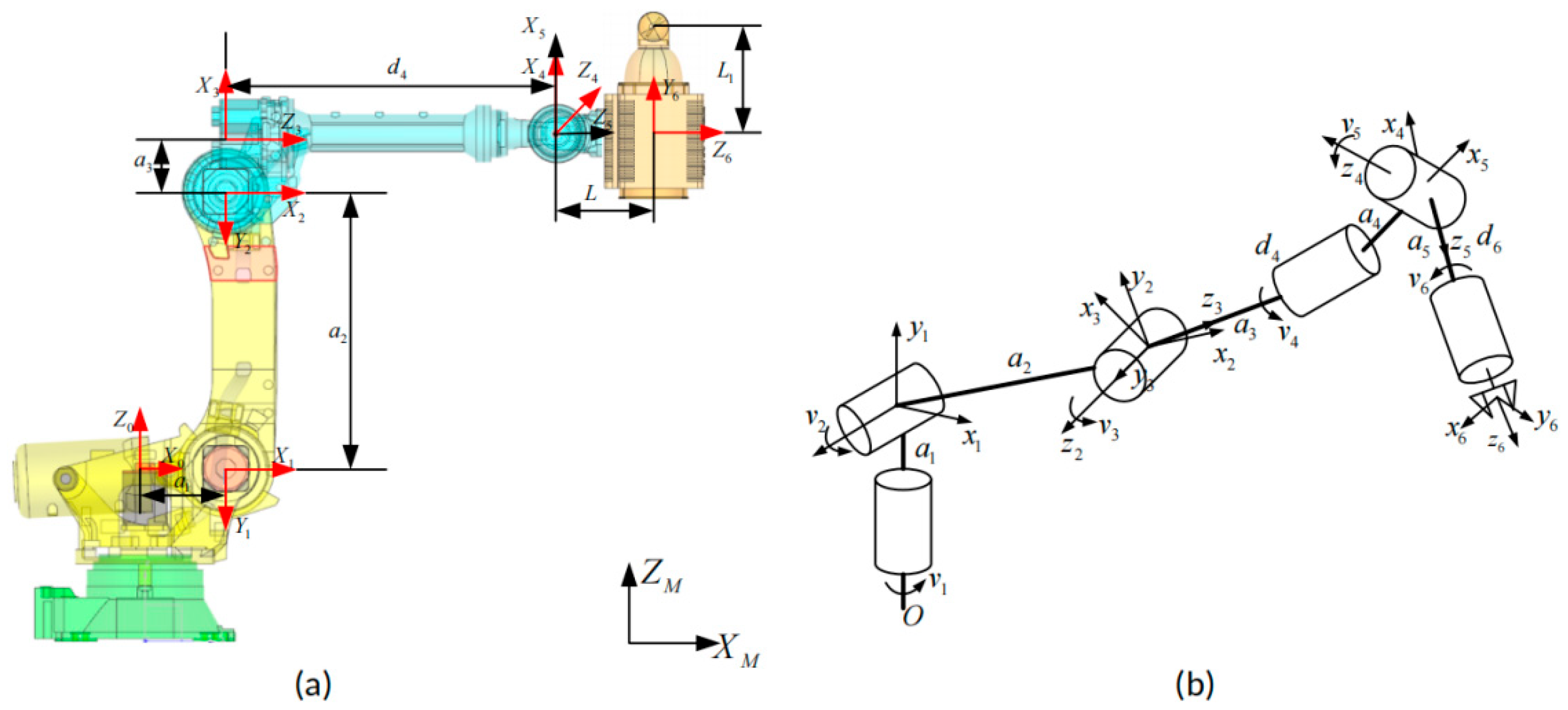
Figure 1. Measurement elements in BIW inspection.
Applsci 15 06181 g001
Figure 2. Key definitions in inspection by Laser Radar.
Applsci 15 06181 g002
Figure 3. (a) The feasible region for a feature; (b) The shared region for multiple features.
Applsci 15 06181 g003
Figure 4. Clustering for features to be measured.
Applsci 15 06181 g004
Figure 5. Discretized spherical regions for feasible region of features to be measured.
Applsci 15 06181 g005
Figure 6. (a) an AAG example; (b) MCSG1 identified from AAG1; (c) an AAG example; (d) MCSG2 identified from AAG2.
Applsci 15 06181 g006
Figure 7. Interference checking of laser beam.
Applsci 15 06181 g007
Figure 8. Collision constraint with ground.
Applsci 15 06181 g008
Figure 9. Collision constraint with BIW.
Applsci 15 06181 g009
Figure 10. (a) A 6-DOF industrial robot; (b) Linkage model of industrial robot.
Applsci 15 06181 g010
Figure 11. (a) Features to be measured; (b) the inspection scene.
Applsci 15 06181 g011
Figure 12. Reachable area of robot’s wrist. (a) Reachable area of wrist. (b) Section view of reachable area. (c) Outer border of reachable area. (d) Inner border of reachable area.
Applsci 15 06181 g012
Figure 13. Optimized stations of Laser Radar.
Applsci 15 06181 g013
Table 1. Parameters about industrial robot’s arms.
No.Distance Between Adjacent Axes (αi)Angle Between Adjacent z Axes (αi)Center Distance of Joint (di)Angle Between Adjacent X Axes (βi)
1α1−π/20β1
2α200β2
3α3−π/20β3
4α4−π/2d4β4
5α5−π/20β5
6α60Lβ6
Table 2. The data on inspection features.
Point Codingx-Coordinatey-Coordinatez-CoordinateNormal Vector iNormal Vector jNormal Vector k
L22A781CRE4233.000−626.6211511.5400.0000.939−0.342
R22A800ECE4881.610−850.327873.5720.399−0.328−0.856
L22A413AFV4789.710−350.1001681.7500.090−0.0700.990
Table 3. Some inspection features with shared feasible regions.
Region 1
Point Codingx-Coordinatey-Coordinatez-CoordinateNormal Vector iNormal Vector jNormal Vector k
L22A818ASV4882.130−282.0001602.000−0.780−0.0300.632
L12A800CSZ3856.000−567.0001680.5100.000−0.1100.990
L22A271AAZ3860.060−598.681703.4000.000−0.2200.970
Region 2
Point Codingx-Coordinatey-Coordinatez-CoordinateNormal Vector iNormal Vector jNormal Vector k
L22A771CRP3392.500704.3451212.2900.000−0.995−0.100499
R22A771ARP3295.200705.7371189.3000.000−0.995−0.100
L22A800ISY3705.500−762.500 480.0000.000−1.0000.000
Region 3
Point Codingx-Coordinatey-Coordinatez-CoordinateNormal Vector iNormal Vector jNormal Vector k
R22A781CRE4234.000623.5491519.9900.000−0.940−0.340
R22A781BCE4214.190605.6001560.620−0.037−0.933−0.358
L12A801FSY1980.000−745.000813.0000.000−1.0000.000
Table 4. Parameters about the R-2000i robot’s arms.
No.Distance Between Adjacent Axes (αi)Angle Between Adjacent z Axes (αi)Center Distance of Joint (di)Angle Between Adjacent X Axes (βi)
1312−π/20β1
2107500β2
3225−π/20β3
40−π/21280β4
50−π/20β5
600500β6
Table 5. Optimized stations of Laser Radar.
Station Codex-Coordinatey-Coordinatez-CoordinateNormal Vector i
14345.480−1450.0003189.0600.000
22951.560−2754.6202111.5800.000
452373.710−1503.1803045.9000.549
Disclaimer/Publisher’s Note: The statements, opinions and data contained in all publications are solely those of the individual author(s) and contributor(s) and not of MDPI and/or the editor(s). MDPI and/or the editor(s) disclaim responsibility for any injury to people or property resulting from any ideas, methods, instructions or products referred to in the content.

