Classification of Tropical Cyclone Tracks in the Northwest Pacific Based on the SD-K-Means Model

Abstract

Tropical cyclone (TC) track clustering plays a crucial role in understanding cyclone movement patterns, which is essential for risk assessment and disaster preparedness. This study proposes an improved SD-K-Means clustering algorithm for classifying TC tracks. Using the best-track datasets of TCs from 2000 to 2022, provided by NOAA (National Oceanic and Atmospheric Administration) and JMA (Japan Meteorological Agency), it explores the quantitative relationships between various TC features, such as latitude, longitude, and wind speed, and their motion speed and deflection angles. Based on these analyses, clustering indicators coupled with TC tracks and motion characteristics are identified. To evaluate the model’s performance, three clustering methods—standard K-Means, DTW (Dynamic Time Warping)-based K-Means, and DBSCAN (Density-Based Spatial Clustering of Applications with Noise)—are compared using the Calinski–Harabasz (CH) index and the Davies–Bouldin Index (DBI) as evaluation metrics. The experimental results show that the SD-K-Means algorithm achieved high consistency across the majority of clustering indices, with the optimal number of clusters determined to be four. The spatial distribution of the clustering results demonstrates that SD-K-Means is effective in distinguishing different TC track patterns, providing valuable insights for regional disaster prevention and risk management efforts.

1. Introduction

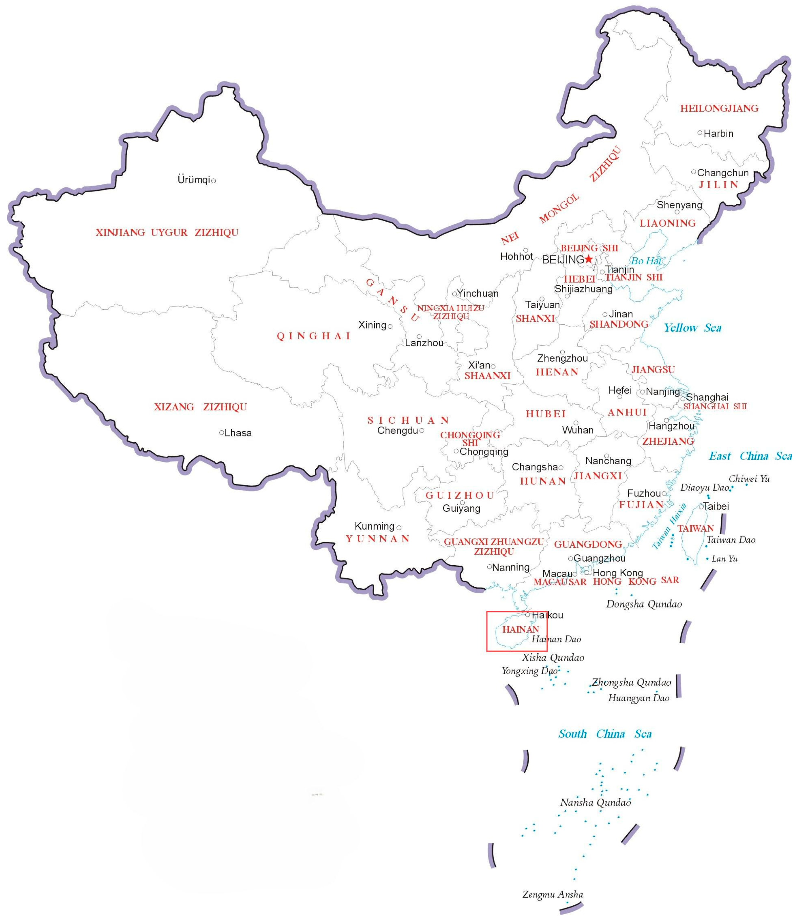
Tropical cyclones (TCs) are extreme marine weather events that can lead to storm surges, flooding, strong winds, and heavy rainfall, posing severe threats to coastal infrastructure and public safety [1,2]. Given China’s extensive coastline, the probability and range of TC impacts are significantly elevated (See Figure 1 for a detailed map of China). Annually, over 20 TCs originating in the western North Pacific (WNP) affect or make landfall along China’s coast, causing substantial losses. Since the 1950s, the direct economic losses from landfalling TCs have increased steadily, surpassing CNY 10 billion by the early 2000s and continuing to grow [3,4]. Moreover, studies indicate that the frequency and intensity of TCs in the WNP have been rising under the influence of global warming [5,6,7]. In this context, understanding TC behavior, predicting landfall regions, and assessing impact potential are crucial for enhancing disaster preparedness and mitigating economic losses and threats to human life.

Whether a TC makes landfall, and its specific landing location, are determined by its track, and its impact extent is governed by the intensity it attains during its evolution. TC tracks are critical for evaluating the potential impact areas and intensity of storms. Classifying TC tracks helps to better understand their characteristics and activity patterns [8]. Common approaches to TC track classification include subjective identification and objective analytical methods. The subjective identification method relies heavily on expert judgment. For example, Huang et al. [9] classified Northwest Pacific (NWP) TCs into four categories based on their genesis locations, activity regions, and dissipation points. However, such methods are highly dependent on human expertise, leading to instability and subjectivity in the classification results.

To overcome these limitations, objective analysis methods grounded in mathematical theory have gained popularity and have become mainstream in recent years. For instance, Elsner [5] utilized a K-Means clustering algorithm based on the longitude and latitude of TC positions at peak intensity and prior to dissipation to classify NWP TCs into straight-moving and northward-bending tracks. However, this approach used only partial location data, thereby underutilizing the complete track information. Building on Elsner’s work, Nakamura et al. [10] employed the HURDAT dataset (Atlantic Basin Historical Hurricane Track Data) and proposed a classification method based on mass moments, including the centroid and variances (radial, latitudinal, and diagonal) of position, intensity, and wind speed. Their dynamic perspective allowed them to cluster Atlantic hurricanes into six distinct types using K-Means. Yu et al. [11] took NWP TCs as the research object. Based on the work of Nakamura et al., they improved the coefficients of five clustering indicators and strengthened the importance of track length, shape, and direction. The above studies focus only on the characteristics of the TC track itself, emphasizing the importance of physical variables, and lack consideration of the changes in physical and spatial characteristics caused by the influence of the environmental flow field during the movement of the TC.

In response to the K-Means clustering algorithm’s limitations—specifically, its insensitivity to temporal characteristics and inability to account for variations in track length—Cammargo et al. [12] proposed a model based on the Finite Mixture Model (FMM). By treating all time-step positions along TC tracks as independent variables and fitting quadratic polynomial regressions, they classified Northwest Pacific TCs from 1950 to 2002 into seven categories using the JTWC (Joint Typhoon Warning Center) dataset. Kim et al. [13] adopted a simple interpolation method combined with the Fuzzy C-Means (FCM) algorithm to retain the approximate track shape and classified NWP TCs into seven categories. They also introduced four validity metrics to determine the optimal number of clusters. Paliwal et al. [14], studying TCs in the North Indian Ocean, compared K-Means and Finite Mixture Models (FMMs), concluding that both produced similar track classifications.

Zhao et al. [15] proposed a similarity threshold learning-based method, combining DBSCAN (Density-Based Spatial Clustering of Applications with Noise) with fastDTW (Fast Dynamic Time Warping) to first identify high-density genesis areas, and then compute similarity between tracks to generate representative paths and classify TCs accordingly. While this approach reduced K-Means randomness and improved classification intelligence, it focused solely on track geometry and ignored the associated physical variables. Similarly, Cai et al. [16] introduced an improved ST-DBSCAN algorithm, combining SS-DBSCAN and DST-DBSCAN, to mitigate DBSCAN’s tendency to mislabel valid samples as noise, focusing on high-intensity and high-landfall-probability regions. However, this model emphasized landfall probability over full lifecycle track analysis. Yin et al. [17] classified South China Sea (SCS) TCs using K-Means and verified its efficacy for regional track studies, though the method remained sensitive to initial cluster numbers and outliers, limiting stability.

To address the above challenges, this study proposes a novel SD-K-Means clustering model, which it applied to TCs formed in the NWP from 2000 to 2022. The model integrates nine clustering indicators—including track similarity and environmental dynamics—to classify TC tracks. The key contributions of this paper are as follows:

(1) Beyond track similarity, this study incorporates dynamic changes caused by environmental flow fields as clustering indicators, improving model performance by capturing the coupled spatial–physical evolution of TCs.

(2) By integrating Soft-DTW—well suited for handling nonlinear, variable-length time series—with K-Means and introducing a cyclic clustering mechanism, the proposed SD-K-Means model reduces classification randomness. Comparative experiments with standard K-Means and DTW-based K-Means validate its superiority.

The remainder of the paper is organized as follows: Section 2 presents the dataset and clustering methodology. Section 3 evaluates the performance of the proposed model against baseline algorithms in terms of accuracy and efficiency. Section 4 analyzes the clustering outcomes and physical characteristics of the resulting TC types, including seasonal trends and potential impacts. Finally, Section 5 summarizes the conclusions of the study.

2. Data and Methods

2.1. Dataset

This study employs the best track datasets for TCs in the NWP (120–180°E, 0–40°N) [18] provided by the National Oceanic and Atmospheric Administration (NOAA) and the Regional Specialized Meteorological Center Tokyo (RSMC-Tokyo) operated by the Japan Meteorological Agency (JMA). These datasets include key TC attributes recorded at 3 h intervals such as the latitude and longitude of the TC center, maximum sustained wind speed, intensity level, and official track forecast errors.

Due to the fact that the JMA began providing official forecast error values only after 2000 and updates remain infrequent, this study focuses on the period from 2000 to 2022. TCs were selected for analysis based on the following criteria: maximum sustained wind speed exceeding 17.2 m/s, assigned international names, and lifespan exceeding 24 h. A total of 507 TCs meeting these criteria were ultimately selected for clustering analysis.

2.2. Clustering Indicators

In addition to data cleaning of the dataset, since this paper takes the speed change and angular deflection amplitude during TC movement as one of the clustering indicators, it was necessary to quantify clustering indicators such as TC speed change and angular deflection amplitude based on the existing characteristic variables of the dataset. Finally, 9 clustering indicators—TC track data, TC intensity level, TC track prediction error, TC life length, TC development length, PDI index, the shortest distance between TC track and the center of Hainan Island, TC moving rate, and TC angular deflection amplitude—were selected for subsequent clustering. The calculation method and brief introduction of the relevant clustering indicators are shown below.

(1)

TC intensity.

Intensity levels from the RSMC-Tokyo dataset are shown in

Table 1. RSMC-Tokyo dataset intensity level description.

TC Level	Name
1	Not used
2	Tropical Depression (TD)
3	Tropical Storm (TS)
4	Severe Tropical Storm (STS)
5	Typhoon (TY)
6	Severe Typhoon (STY)

. Level 1 is excluded; levels 2 through 6 are used in clustering.

(2)

TC track prediction error.

The TC track prediction error uses the official error value provided by the Japan Meteorological Agency, which provides 24, 48, 72, 96, and 120 h path prediction error values for TCs from 2000 to 2022. This paper selects the 24 h official prediction error as the clustering indicator.

(3)

TC life span and TC development span.

The TC life span can reflect the length of the TC track on a time scale. This paper considers only TCs with a life span greater than 24 h. Its calculation method is shown in Equation (1). The TC development span can reflect the length of the TC from generation to reaching TY intensity on a time scale. Its calculation method is shown in Equation (2).

$$L=n-1$$

(1)

$$D=i_T-i_1$$

(2)

Among them, $L$ represents the life span of TC, $D$ represents the development length of TC, $i_T$ represents the moment when TC intensity reaches TY for the first time, and $i_1$ represents the moment when TC is generated.

(4)

PDI (Power Dissipation Index).

The PDI [5] comprehensively considers the maximum wind speed and duration of a TC. This index can reflect the destructive potential of a TC and can be calculated using Equation (3).

$$PDI={\int }_0^{n\int }{V}_{max}^3$$

(3)

where $V_{max}$ represents the maximum wind speed, and the unit of time step $dt$ is $s$.

(5)

The shortest distance between the TC track and the center of Hainan Island.

The shortest distance between the TC track and the center of Hainan Island is calculated by the spherical distance [19], which can be calculated using Equation (4). Since the main research object of the subsequent study is Hainan Province, it is used as one of the clustering indicators in this paper.

$$\Delta d=R\times \mathit{arccos}\left[\mathit{sin}{x}_1\mathit{sin}{x}_2+\mathit{cos}{x}_1\mathit{cos}{x}_2\mathit{cos}\left(y_1-y_2\right)\right]$$

(4)

where $R$ represents the radius of the earth, which is generally 6371 km, and $x_i$ and $y_i$ represent the longitude and latitude of the TC at the $i$-th moment, respectively.

(6)

TC movement speed.

The mutation of TC movement speed is one of the important parameters in TC track research. Therefore, this paper selects the deviation degree of TC movement speed in the entire lifecycle as the clustering index to measure the mutation of TC movement speed. The calculation method is shown in Equation (5).

$$a={\displaystyle \frac{\sqrt{{\sum }_{i=1}^n{\left(v-\stackrel{-}{v}\right)}^2}}{n-1}}$$

(5)

(7)

TC angle deflection amplitude.

The angle mutation of a TC during its movement is also one of the important parameters in TC track research. Therefore, this paper quantifies the angle deflection amplitude of TC throughout its lifecycle and uses it as a clustering index. The calculation method is shown in Equation (6).

$$\beta ={\displaystyle \frac{{\sum }_{i=1}^{n-2}\alpha \left(m\right)}{n-2}}$$

(6)

The sum of the $n-2$ angles is taken as ${\displaystyle \frac{1}{n-2}}$ to ensure that the TC turning amplitude is independent of the TC life span, and $\alpha \left(m\right)$ represents the angle between two adjacent slope segments, which can be calculated by Equation (7).

$$\alpha \left(m\right)=-\mathit{arctan}\left[{\displaystyle \frac{k\left(j+1\right)-k\left(j\right)}{1+k\left(j\right)\times k\left(j+1\right)}}\right]\begin{array}{cc},& m=\mathrm{1,2},\dots ,n-2\end{array}$$

(7)

The negative sign is to ensure that the clockwise steering angle $\alpha$ is positive, and $k\left(j\right)$ represents the slope of the TC track between two adjacent moments, which can be calculated by Equation (8).

$$k\left(j\right)={\displaystyle \frac{y_{i+1}-y_i}{x_{i+1}-x_i}}\begin{array}{cc},& j=\mathrm{1,2},\dots ,n-1\end{array}$$

(8)

Finally, normalization was performed to eliminate the dimensional differences between different clustering indicators.

2.3. Clustering Method

2.3.1. K-Means Clustering Algorithm

The K-Means clustering algorithm is a commonly used distance-based clustering algorithm. It achieves the clustering goal by minimizing the Sum of Squared Error (SSE), that is, obtaining the minimum sum of the squares of the distance from each sample point to the center of its cluster. Its calculation formula is shown in Equation (9).

$$SSE=\sum _{i=1}^K\sum _{x\in C_i}{‖x-{\mu }_i‖}^2$$

(9)

where $K$ represents the number of clusters, $C_i$ represents the set of sample points in the $i$-th cluster, $x$ represents the sample point in $C_i$, ${\mu }_i$ represents the centroid of the $i$-th cluster, and ${‖x-{\mu }_i‖}^2$ represents the square of the Euclidean distance between the sample point $x$ and the cluster center ${\mu }_i$. Euclidean distance is the default method used by the K-Means clustering algorithm to measure the distance from the sample point to the cluster center. Its calculation method is shown in Equation (10).

$$d\left(x,\mu \right)=\sqrt{\sum _{j=1}^n{\left(x_j-{\mu }_j\right)}^2}$$

(10)

The working principle of the K-Means clustering algorithm is to randomly select $K$ samples as the initial cluster center, then calculate the distance between each sample and the initial cluster center, and classify each sample into the cluster with the smallest distance based on the obtained distance. After completing the division of each sample, each cluster starts a new round of iteration, that is, re-find the cluster center and calculate the clustering of each sample with the new cluster center so as to re-cluster each sample. This iterative process is repeated until the cluster center no longer changes, that is, the distance between samples in each cluster reaches the maximum value.

2.3.2. Soft-DTW Algorithm

Dynamic Time Warping (DTW) is a common method for measuring the similarity of time series. Compared with direct measurement methods such as Euclidean distance, the DTW algorithm can handle nonlinear time changes in time series signals, that is, it can handle time offsets and length differences, and its effect is relatively good among a number of time series similarity calculation methods (for example, Longest Common Subsequence (LCSS) and Edit Distance for Real Sequences (EDR)).

The DTW algorithm matches time series by stretching and compressing the nonlinear time axis to measure the similarity between the time series. Its essence is to find the optimal alignment path between two time series through dynamic programming to minimize the distance between them. If two time series $X=\left(x_1,x_2,\dots ,x_{n-1},x_n\right)$ and $Y=\left(y_1,y_2,\dots ,y_{m-1},y_m\right)$ are given, the calculation equation of DTW can be expressed as follows:

$$D\left(i,j\right)=d\left(x_i,y_j\right)+\mathit{min}\left\{DTW\left(i-1,j\right),DTW\left(i,j-1\right),DTW\left(i-1,j-1\right)\right\}$$

(11)

where $D\left(i,j\right)$ represents the DTW distance between subsequences $X\left[1:i\right]$ and $Y\left[1:j\right]$, $d\left(x_i,y_j\right)$ represents the distance between $x_i$ and $y_j$, and the DTW distance between sequences $X$ and $Y$ is $D\left(n,m\right)$.

At the same time, to reduce the size of the search space and find the optimal alignment path faster, it needs to meet the following five restrictions: first, monotonicity, that is, the path is unidirectionally corresponding and the features are not repeated in the path; second, continuity, that is, the path cannot jump, ensuring that no feature is skipped; third, boundary conditions, that is, the path starts from the upper left and ends at the lower right, ensuring that both time series are considered as a whole; fourth, regular window, that is, ensuring that the path with the shortest distance is selected when corresponding features; fifth, slope restriction, that is, preventing two time series with too long lengths from being matched.

However, the DTW algorithm is discrete and non-differentiable, and its robustness is poor. To solve the above problems, a Soft-DTW (Soft Dynamic Time Warping) algorithm [20] that uses a smoother DTW distance to measure the similarity between two time series has emerged. The calculation equation of the Soft-DTW algorithm can be expressed as follows:

$$DTW\left(X,Y\right)={\mathit{min}}^{\gamma }\left\{D\left(n,m\right)\right\}=-\gamma \mathit{log}\left(\sum _{\pi }{e}^{-{\displaystyle \frac{D_{\pi }}{\gamma }}}\right)$$

(12)

where $\pi$ represents all possible paths, $\gamma$ represents the smoothing parameter ($\gamma >0$). When $\gamma$ tends to 0, Soft-DTW degenerates into standard DTW; when $\gamma$ increases, the path becomes smoother.

2.3.3. DBA Algorithm (DTW Barycenter Averaging)

The DBA (Dynamic Time Warping Barycenter Averaging) algorithm can calculate the geometric center of a given set of time series data to obtain the average time series of a set of time series. At the same time, compared with the traditional arithmetic average method, the DBA algorithm takes into account the intrinsic structure of the time series data and retains its core features, that is, it is more accurate and more stable than traditional algorithms in the problem of time series alignment.

The working principle of this algorithm can be summarized as aligning each time series to a selected reference sequence and averaging the aligned sequences. Specifically, first select a reference time series, which is generally randomly selected, and then align each time series to the reference sequence by calculating the distance between each time series and the reference sequence, and finally, average the aligned sequences to obtain an average sequence that can represent the group of time series. Then, the above process is repeated iteratively until the average sequence of the entire group of time series converges.

2.3.4. SD-K-Means Clustering Algorithm

TC track data are a typical time series. The DTW algorithm can be used to quantify the similarity between TC tracks, thereby realizing the clustering of TC tracks. However, some TCs may have singular points in their tracks or the appearance of circular tracks due to sudden changes in speed or direction, that is, there are situations where local changes are large. The DTW algorithm is less sensitive to such situations, which may affect the clustering effect, but Soft-DTW allows local inaccurate matching and is more robust to changes. At the same time, TC tracks belong to nonlinear time series of varying lengths. Compared with DTW, Soft-DTW is more suitable for clustering problems of such sequences. In addition, the Soft-DTW algorithm supports optimizing cluster centers by gradient descent, and the clustering effect can be optimized by adjusting the smoothing parameter $\gamma$ introduced. In summary, this paper finally selected Soft-DTW to measure the similarity between TC tracks and proposed the SD-K-Means clustering model in combination with the K-Means clustering algorithm to cluster 507 TCs generated in the Northwest Pacific from 2000 to 2022.

The main workflow of TC track clustering based on the proposed SD-K-Means clustering model is as follows:

(1)

Compute the Soft-DTW distance matrix and the matrix of normalized TC features. The Soft-DTW clustering matrix and the TC feature information matrix are obtained based on the TC track data and the clustering index based on the quantification of TC feature variables, and they are combined as the input of the model.

(2)

Initialize cluster centers randomly. Assign each TC to the cluster with the nearest center using Soft-DTW.

(3)

Update the cluster center using the DBA algorithm. Since the Soft-DTW algorithm does not have the concept of explicit mean, the DBA algorithm is used to calculate the track mean as the new center track. Its alignment method is set to “softdtw”, that is, the Soft-DTW algorithm is used to align the sequence, and then the above process is continuously iterated until the clustering result is stable.

(4)

To mitigate the randomness of center initialization, the clustering is repeated 1000 times.

There are two commonly used methods for determining the optimal number of clustering categories $K$: the Elbow Method and the Silhouette Coefficient Method. Among them, the Silhouette Coefficient Method comprehensively considers the compactness within the cluster and the separation between clusters and measures the clustering effect by calculating the silhouette coefficient. The specific calculation equation is shown in Equation (13).

$$S_i={\displaystyle \frac{min\left(b_i\right)-a_i}{max\left[a_i, min{b}_i\right]}}$$

(13)

where $S_i$ represents the silhouette coefficient score of the $i$-th sample, and its value range is −1~1; $a_i$ represents the average distance from the i-th sample to other samples of the same category; and $b_i$ represents the average distance from the i-th sample to all samples outside the category. The closer the value of $S_i$ is to 1, the better the clustering effect is. The closer the value of $S_i$ is to 0, the worse the clustering effect is. The closer the value of $S_i$ is to −1, the more it means that the sample i is misclassified and should belong to other categories.

The elbow rule measures the quality of clustering results under different $K$ values by calculating the SSE of each cluster under different $K$ values, that is, calculating the sum of squared distances between each sample and the cluster center of the cluster to which it belongs. The specific calculation equation is shown in Equation (10). The smaller the SSE value, the tighter the clustering result, that is, the better the clustering effect. 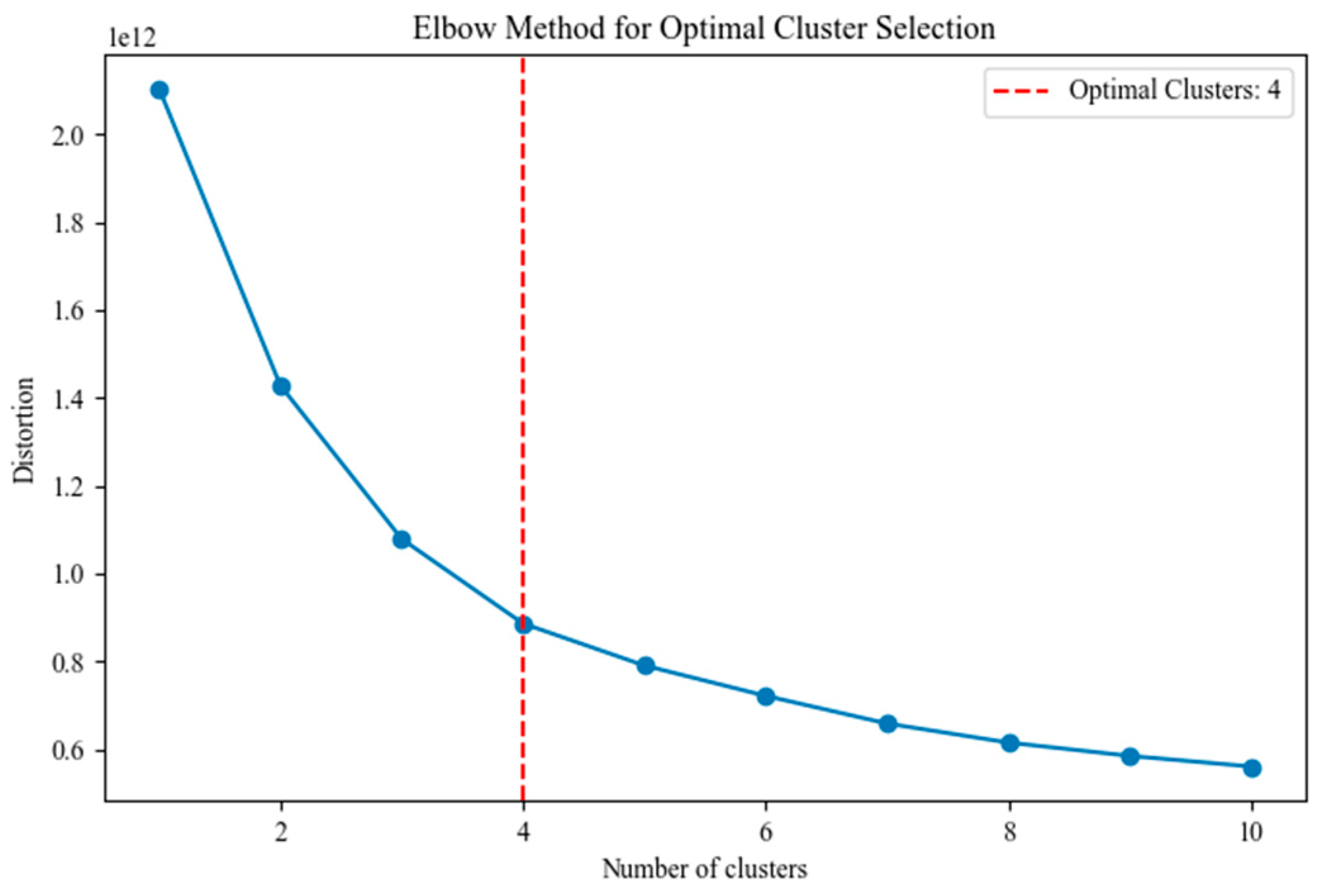However, in reality, as the $K$ value continues to increase, the SSE value will continue to decrease. Considering factors such as time cost, the $K$ value at the “elbow” position where the gain is smaller, that is, the SSE value decreases slowly, is usually selected as the optimal $K$ value. This paper chooses to use the elbow method and determines the optimal $K$ value by the average SSE value of 1000 clustering cycles, that is, the average value of the SSE values of 1000 clustering cycles. The specific SSE value results under different $K$ values are shown in Figure 2.

As can be seen from Figure 2, the change in the slowdown of the decline occurs when $K=4$; that is, when the TC tracks are divided into 4 categories, the clustering effect of the SD-K-Means clustering model is optimal.

3. Model Performance

To evaluate the performance of the proposed clustering model and to compare it with alternative approaches, this study employs two widely used internal validation metrics: the Calinski–Harabasz (CH) index and the Davies–Bouldin index (DBI). These metrics are used to assess the clustering results of four different algorithms: the proposed SD-K-Means model, the DTW-based K-Means model, the standard K-Means algorithm, and DBSCAN.

The CH index, also known as the variance ratio criterion, evaluates clustering quality based on the ratio of between-cluster dispersion to within-cluster compactness. Its formulation is given in Equation (14):

$$CH={\displaystyle \frac{S{S}_B}{K-1}}/{\displaystyle \frac{S{S}_W}{n-K}}={\displaystyle \frac{tr\left(B_K\right)}{tr\left(W_K\right)}}\times {\displaystyle \frac{n-K}{K-1}}$$

(14)

where $n$ represents the number of samples, $K$ represents the number of clusters, $S{S}_B$ represents the variance between clusters, $S{S}_W$ represents the variance within clusters, $B_K$ represents the distance between clusters, and $W_K$ represents the distance within clusters.

In essence, a higher CH index implies that the clusters are more distinct (greater inter-cluster separation) and internally more cohesive (smaller intra-cluster variance). Thus, larger CH index values indicate better clustering performance. The specific CH index values of the SD-K-Means clustering model, the DTW-based K-Means clustering model, and the K-Means clustering model are shown in

Table 2. Comparison of CH index values of multi-clustering models.

Clustering Model	K-Means	DBSCAN	DTW-Based K-Means	SD-K-Means
CH Index	122.7050	173.1103	221.8391	230.3705

.

As shown in Table 2, the SD-K-Means model achieves the highest CH index (230.3705), indicating the best clustering performance among the four models. In contrast, the K-Means model shows the lowest CH index (122.7050), suggesting the poorest performance in separating and compacting clusters.

DBI, also known as the classification accuracy index, is also an evaluation index for measuring the quality of clustering effects. It comprehensively considers the similarity of samples within the cluster and the difference in samples between clusters. A lower DBI value indicates that clusters are compact and well separated. The DBI is defined as follows:

$$DBI={\displaystyle \frac{1}{n}}\sum _{i=1}^{n}max{\displaystyle \frac{\overline{S_i}+\overline{S_j}}{{‖w_i-w_j‖}_2}}, i\ne j$$

(15)

where, $\overline{S_i}$ represents the average distance from the $i$-th cluster sample to its cluster center, and ${‖w_i-w_j‖}_2$ represents the Euclidean distance between the $i$-th cluster and the $j$-th cluster center.

The specific DBI values of the SD-K-Means clustering model, the DTW-based K-Means clustering model, and the K-Means clustering model are shown in

Table 3. Comparison of DBI values of multi-clustering models.

Clustering Model	K-Means	DBSCAN	DTW-Based K-Means	SD-K-Means
DBI	1.6221	0.9268	1.2229	1.1422

.

As observed in Table 3, the K-Means model again performs the worst, yielding the highest DBI value (1.6221), indicating poor intra-cluster cohesion and inter-cluster separation. The SD-K-Means model achieves a relatively low DBI of 1.1422, outperforming the DTW-based K-Means model (1.2229), although slightly underperforming compared with DBSCAN (0.9268).

However, when considering both metrics in combination, the SD-K-Means model demonstrates a more balanced and superior performance. The high CH index coupled with a relatively low DBI suggests that the SD-K-Means algorithm produces clusters that are both well separated and internally cohesive, making it more robust than the other models in handling the nonlinear and variable-length nature of TC tracks.

Notably, the DBSCAN model exhibits the lowest DBI, indicating its tendency to form highly compact clusters. However, this may come at the cost of over-segmentation and potential overlap among cluster characteristics. In contrast, the SD-K-Means model balances cluster compactness and separation more effectively, confirming its overall superiority in clustering tropical cyclone tracks.

4. Results Analysis

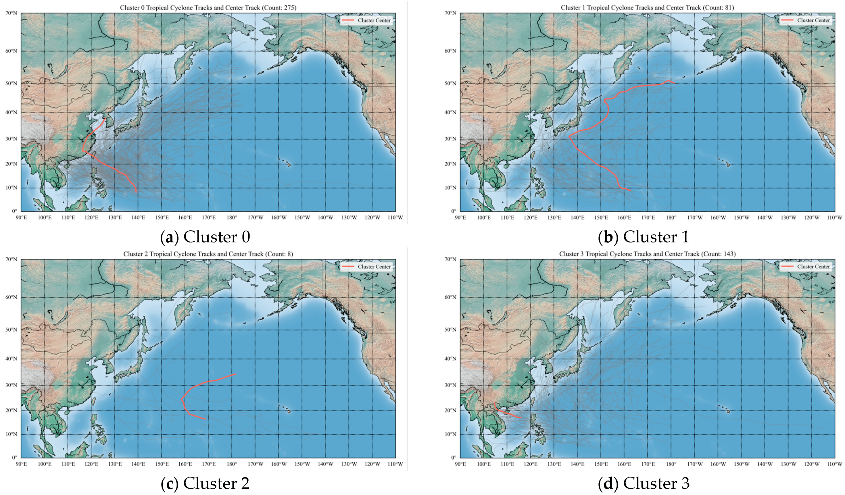
The proposed SD-K-Means clustering model divides TC tracks in the NWP between 2000 and 2022 into four distinct categories, labeled as Cluster 0, Cluster 1, Cluster 2, and Cluster 3. The specific classification outcomes are presented in Figure 3, with the number of TCs per cluster as follows: Cluster 0 contains 274 TCs, Cluster 1 contains 79 TCs, Cluster 2 includes 8 TCs, and Cluster 3 comprises 146 TCs.

Each cluster exhibits distinct track patterns and characteristics. The following sections provide a detailed analysis and interpretation of the clustering results.

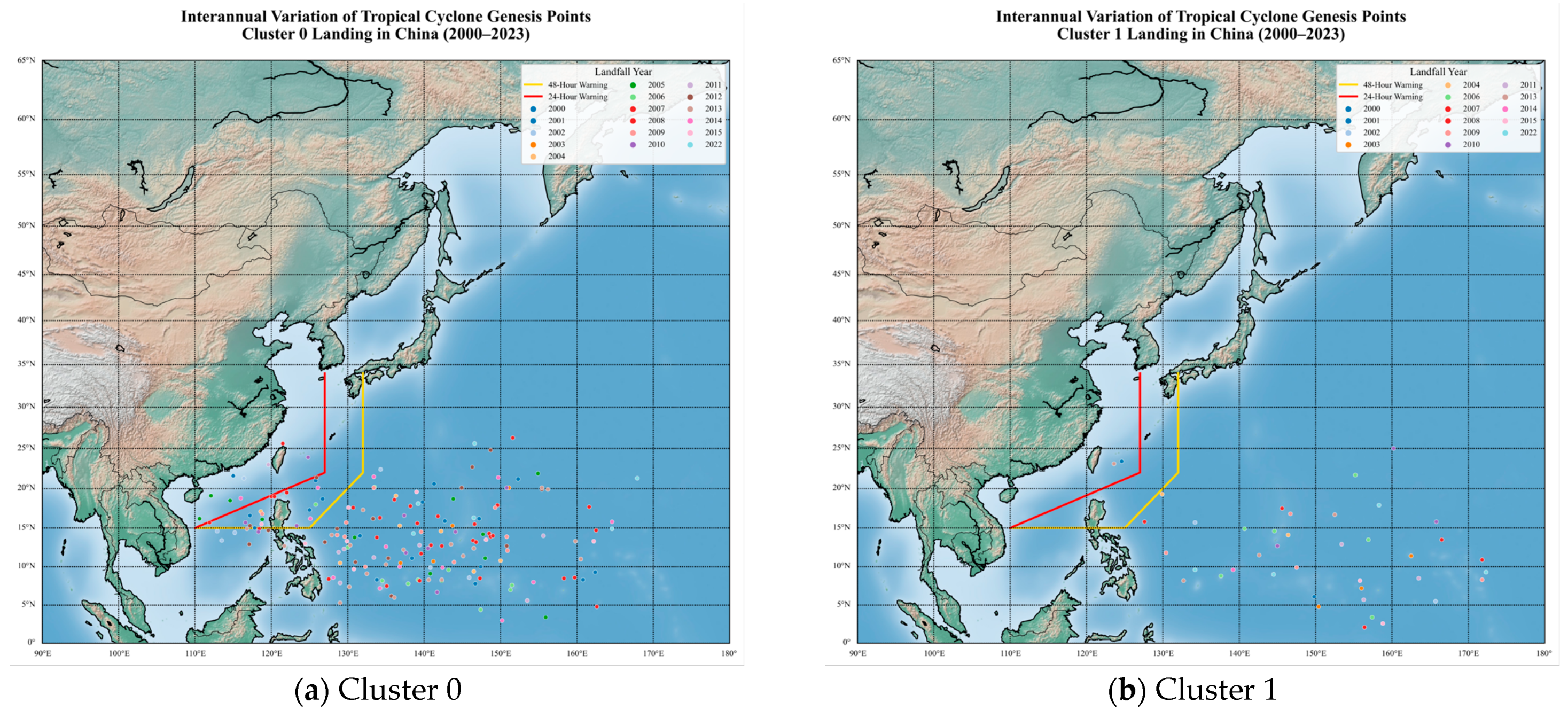
Cluster 0: This cluster primarily consists of TCs that exhibit two main patterns:

TCs that follow the first pattern are generated in the NWP and land on Hainan Island; or they turn near eastern China, initially move westward before curving northeastward near 20–30° N and 120–125° E, typically along the eastern coast of China. These TCs often impact northeastern China, the Korean Peninsula, and Japan. TCs following the second pattern, generally forming in the NWP around 130–140° E, move westward across the SCS and primarily impact Hainan, Guangdong, Vietnam, and Laos. In terms of intensity, TCs in this cluster exhibit moderate growth and shorter durations of maximum intensity compared with those in Cluster 1.

Cluster 1: This cluster is composed almost entirely of turning-type TCs. These TCs also exhibit initial westward movement, followed by a turn to the northeast. However, from the position of the central track in Figure 4, it can be found that compared with the turning TCs in Cluster 0, the deflection positions of the turning TCs in this category are mostly near 20~30° N and 125~135° E, which are relatively further east, that is, relatively farther from the eastern coastline of China, and the straight distance to the west is shorter. From the perspective of activity and impact areas, TCs in this category mostly affect the Korean Peninsula and Japan. These TCs originate further east in the NWP (140–170° E). Compared with Cluster 0, they show faster intensification and longer periods of high intensity, indicating stronger storm systems overall.

Cluster 2: This cluster contains the fewest TCs. These storms are typically generated east of 150° E in the central Pacific and rarely impact the Chinese coast. Most remain over the open ocean, though some may influence Japan. These TCs are among the strongest in terms of intensity and destructive potential.

Cluster 3: Cluster 3 includes two typical TC types: Northeastward-moving TCs and Hainan-landfalling TCs formed in the SCS. The northeastward-moving TCs originate in the central NWP (east of 130° E) and primarily impact Japan. The Hainan-bound TCs, generated in the SCS (west of 120° E), travel westward without turning and mainly affect Hainan, Guangdong, Vietnam, and Laos. From an intensity perspective, TCs in this cluster display slower intensification and shorter durations of peak intensity, especially for those making landfall in Hainan, which tend to be weaker and shorter-lived.

Next, this chapter analyzes the four types of TCs from multiple aspects, such as TC intensity and destructive potential, activity season, and landing situation. At the same time, since the subsequent research is based on Hainan Province, this chapter also analyzes the clustering of TCs that land in Hainan separately.

4.1. TCs’ Intensity and Destructive Potential

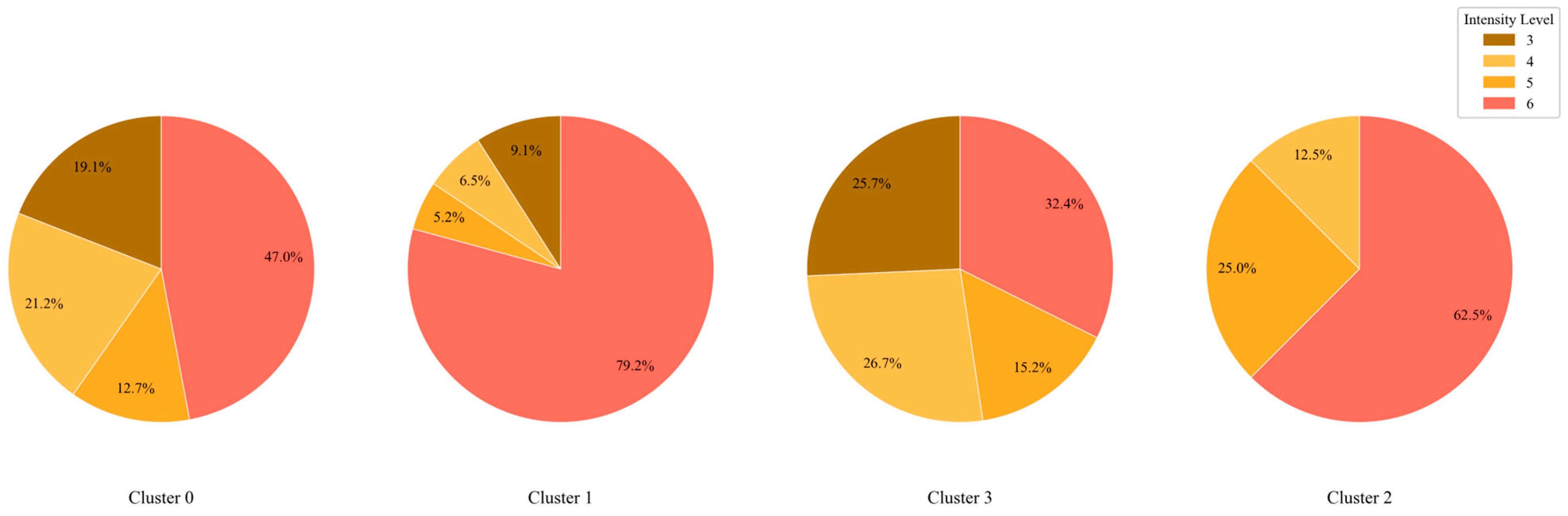
To better visualize intensity differences across clusters, Figure 5 presents the distribution of TC intensity levels categorized according to the RSMC-Tokyo standard. The legend provides corresponding color codes.

As shown, Clusters 1 and 2 contain the strongest TCs, with over 50% of the TCs reaching intensity level 6 or higher. Cluster 2, in particular, exhibits a minimum intensity of level 4, with no weak storms. Nearly half of the TCs in Cluster 0 also reach level 6, while Cluster 3 exhibits a relatively uniform and lower intensity distribution, classifying it as the weakest cluster overall.

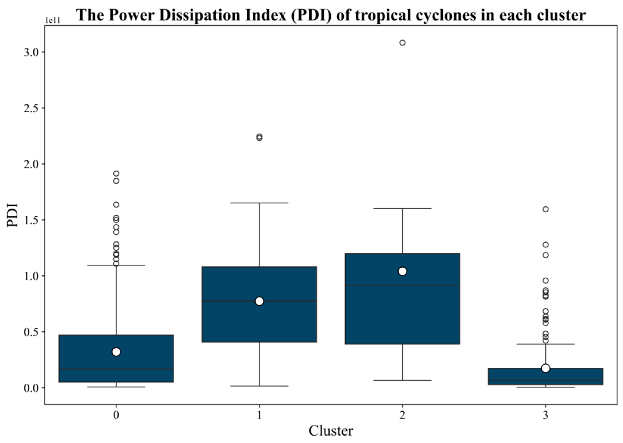
Given the established correlation between TC intensity and destructive power, the PDI is used to further assess and compare the potential destructiveness of the TCs in each cluster. A higher PDI indicates greater accumulated energy, and thus, stronger destructive potential.

From Figure 6, it is evident that Cluster 2 TCs have the highest mean and median PDI, signifying the greatest destructive potential. Cluster 1 ranks second, with a slightly lower but comparable mean PDI. Cluster 0 shows moderate destructive potential. Cluster 3 exhibits the lowest PDI, aligning with its classification as having the weakest storms. These findings are consistent with the intensity-level distributions shown in Figure 5 and validate the clustering model’s ability to distinguish TCs with varying impacts and characteristics.

4.2. TC Activity Season

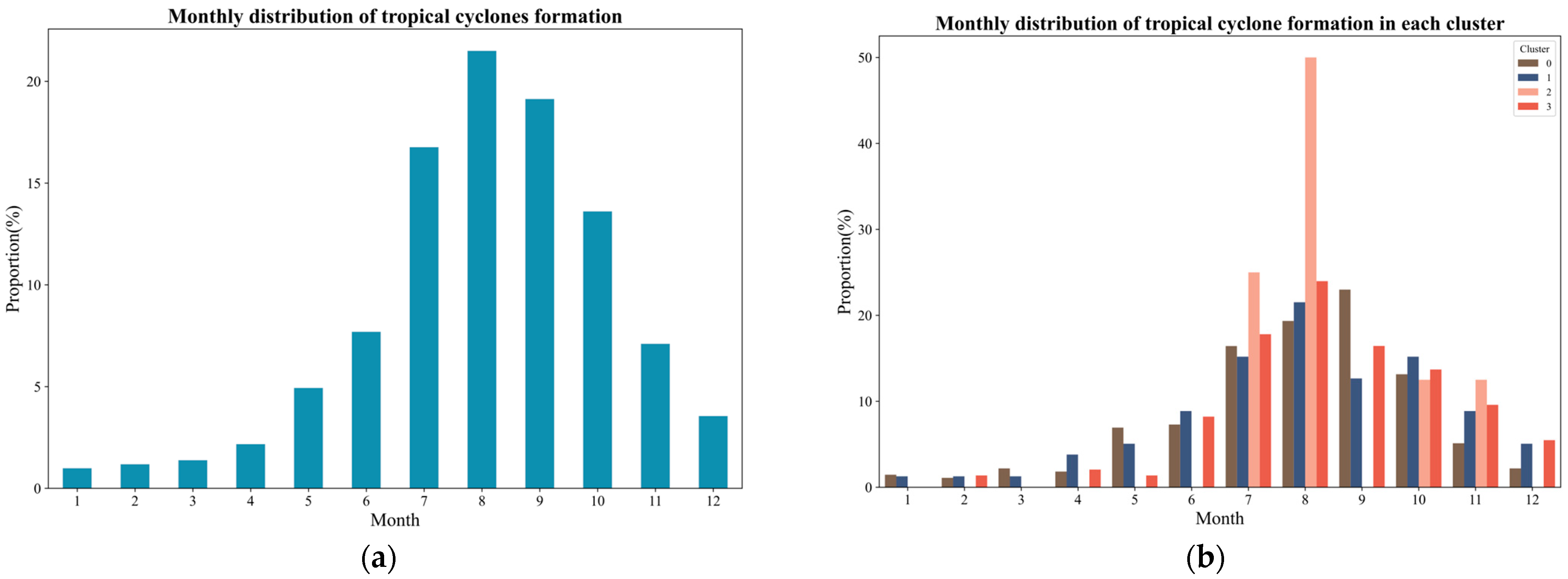
Through the analysis and introduction of various TCs in the previous section, it is evident that there are differences in the activity ranges of these TCs. This discrepancy may arise because the activity seasons of different TCs vary, leading to distinct effects from the environmental flow fields in the relevant sea areas (such as subtropical high pressure, monsoon trough, etc.). To test this hypothesis, this paper visualizes the average monthly active distribution of TCs throughout the year (calculated using monthly TC generation data from 2000 to 2022) along with the average monthly active distribution of various types of TCs annually. The specific distribution is illustrated in Figure 7.

As illustrated in Figure 7a, TCs can form in the NWP throughout the year, though the peak period primarily spans from July to October. This seasonal peak is mainly due to the northward and intensified extension of the subtropical high during summer, which enhances convergence and upward motion in the intertropical convergence zone and the monsoon trough—conditions favorable for TC genesis. In autumn, although the influence of the subtropical high-pressure system weakens as it begins to retreat eastward and move southward, its residual influence remains considerable. Furthermore, the ocean retains substantial heat from solar radiation accumulated during summer, resulting in persistently warm sea surface temperatures in early autumn, which further promotes TC formation [21,22,23,24,25]. Figure 7b presents the seasonal activity distribution by cluster. Despite histogram distortion caused by the unequal sample sizes across clusters, the seasonal activity trends generally align with the overall pattern. The absence of Cluster 2 activity in many months is likely due to its small sample size, yet in the months where TCs do form, its seasonal curve remains consistent with the general trend. Interestingly, Cluster 1 exhibits relatively low activity in September, deviating from the typical seasonal pattern. This anomaly may be associated with anomalous environmental factors such as unusually strong and westward-extending subtropical highs, premature retreat of the SCS monsoon (resulting in insufficient moisture and energy), or enhanced vertical wind shear disrupting the vertical structure of developing TCs [26,27].

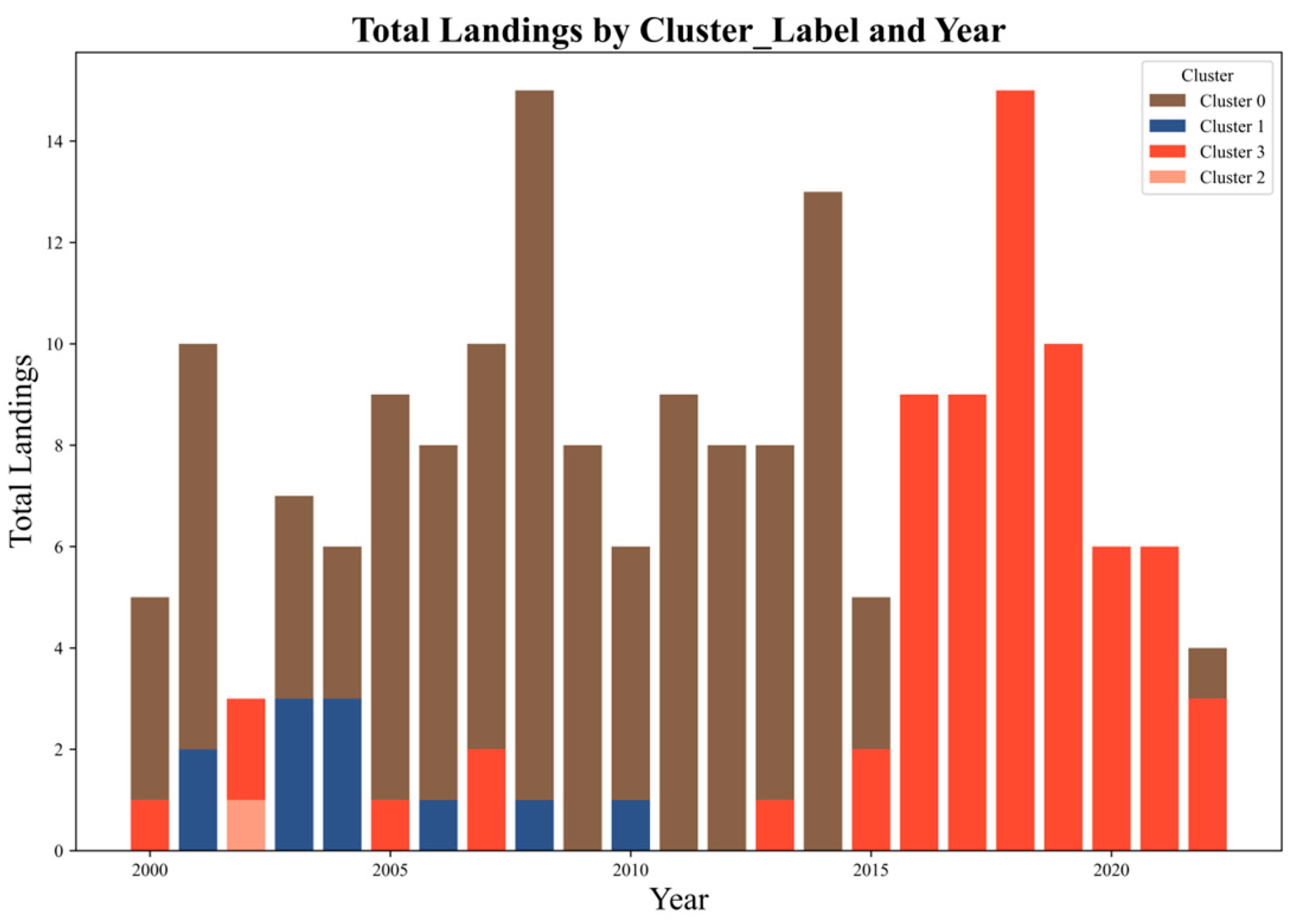
4.3. TC Landing Situations

Although TCs will continue to affect surrounding areas during their movement and thus cause losses to coastal areas, the damage they cause to the landing point and its surrounding areas when they land is particularly huge. Therefore, this section visualizes the annual landing situations of various TCs [28,29]. The specific landing statistics are shown in Figure 8.

As can be seen from Figure 8, in the 23 years from 2000 to 2022, Cluster 0 consistently exhibits the highest proportion of landfalling TCs, accounting for the majority in over 72.7% of the years. According to Figure 3, these TCs primarily make landfall in the eastern coastal provinces of China. In the remaining years, Cluster 3 accounts for the most landfalling TCs, primarily affecting southeastern coastal regions such as Hainan and Guangdong Provinces. Clusters 1 and 2 contribute relatively fewer landfalling TCs, and their impacts are mainly confined to the Korean Peninsula and Japan.

To further illustrate landfall behavior, the yearly distribution of TC genesis locations in each cluster is shown in Figure 9. Notably, from 2016 to 2021, only Cluster 3 TCs made landfall, consistent with the simplified bar chart pattern seen during this period in Figure 8.

A provincial breakdown of landfall occurrences in China is provided in

Table 4. Proportion of TCs making landfall in China’s coastal provinces (%).

Category	Liaoning	Shandong	Jiangsu	Shanghai	Zhejiang	Fujian	Guangdong	Guangxi	Hong Kong	Hainan	Taiwan
Cluster 0	1	80	1	1	65	69.4	60.7	57.1	1	50	70.7
Cluster 1	0	20	0	0	10	8.3	4.9	0	0	0	12.2
Cluster 2	0	0	0	0	5	0	0	0	0	0	0
Cluster 3	0	0	0	0	20	22.2	34.4	42.9	0	50	17.1
Total (Number)	2	5	1	4	20	36	61	7	3	32	41

. The results confirm that southeastern coastal regions—specifically Guangdong, Taiwan, Fujian, and Hainan Provinces—are most frequently impacted by landfalling TCs. In contrast, northeastern regions experience fewer landfalls. Most landfalling TCs fall under Clusters 0 and 3, which is consistent with earlier observations.

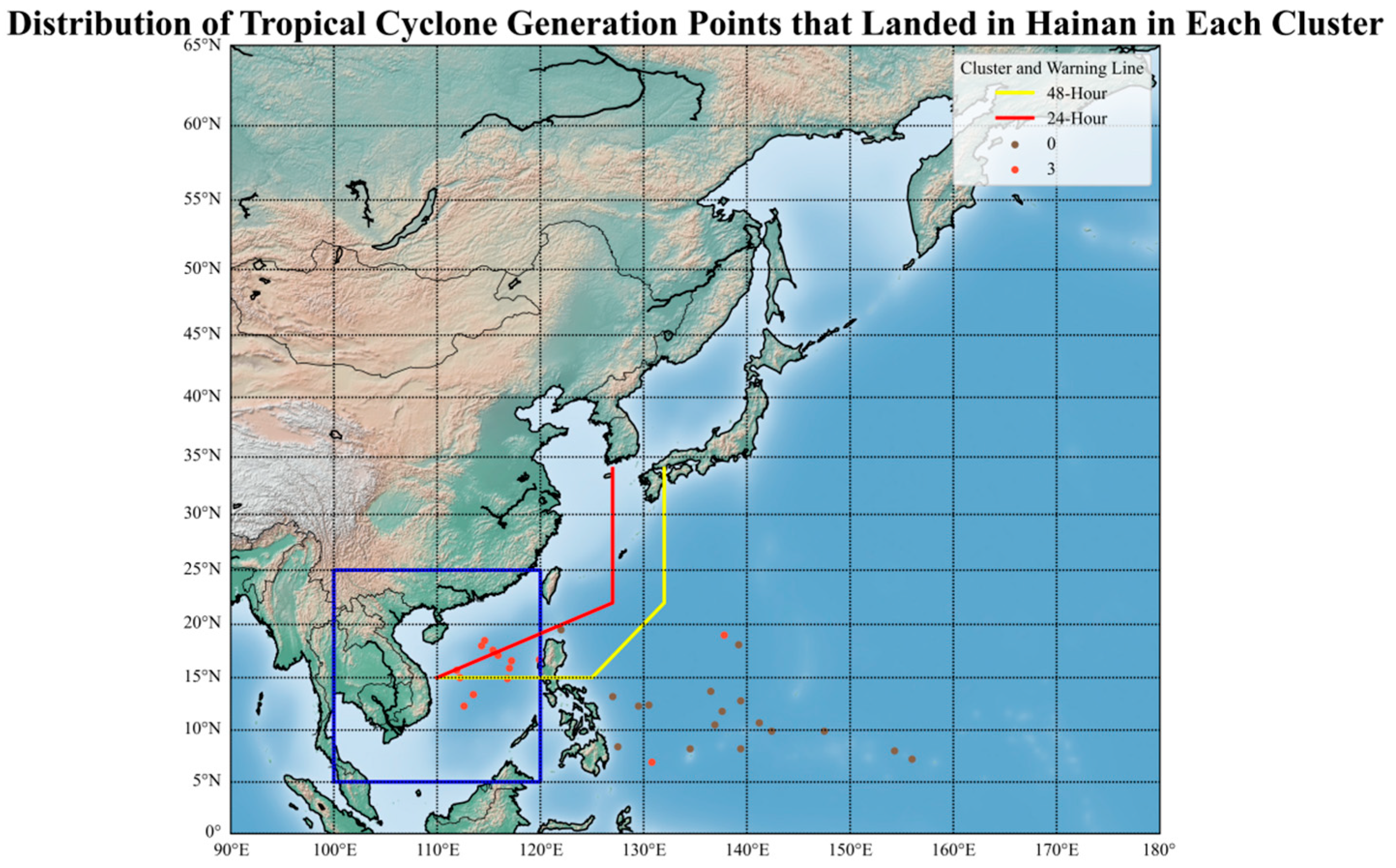
4.4. TCs Making Landfall in Hainan

Given the focus of subsequent research on Hainan Province, this section specifically analyzes TCs that made landfall in Hainan. The genesis locations of these TCs are visualized in Figure 10. The yellow and red lines denote the 24 h and 48 h warning lines, respectively, while the blue box indicates the SCS domain, providing geographic context for classification outcomes.

As shown in Figure 10, TCs that made landfall in Hainan and originated from the Northwest Pacific were mostly classified into Cluster 0, while those originating in the SCS were exclusively classified into Cluster 3. Only two TCs generated in the Northwest Pacific were assigned to Cluster 0. Further analysis of the clustering results and associated tracks is presented in Figure 11. Meanwhile, Figure 12 visualizes the center average trake of each cluster.

According to Table 4, all TCs making landfall in Hainan belonged to either Cluster 0 or Cluster 3. As illustrated in Figure 11, the two TCs generated in the Northwest Pacific but classified into Cluster 0 were relatively weak before entering the SCS, where they intensified to TS strength or higher. In general, TCs that originated in the NWP and later made landfall in Hainan had longer development periods, greater intensities, and longer durations of high intensity compared with those formed within the SCS.

5. Conclusions

This study proposes an improved SD-K-Means clustering model for the classification of TC tracks. Using TC track data from 2000 to 2022, the model integrates key track characteristics such as movement speed and directional changes, thereby enhancing its capability to describe track morphology and improving the rationality of the clustering results. Experimental comparisons demonstrate that the proposed method outperforms traditional K-Means, DTW-K-Means, and DBSCAN algorithms in terms of mainstream evaluation metrics, including the CH index and DBI, verifying its effectiveness and superiority in TC track pattern recognition. Based on the optimal clustering results, the characteristics of different TC clusters were further analyzed, leading to the following main conclusions:

(1)

Track Typology: TCs were classified into four distinct clusters—those turning near the east of China and those generated in the NWP and landing in Hainan, those moving straight in the northeast and those generated in the SCS and landing in Hainan, and those turning and those of a few. These clusters show clear differences in spatial activity ranges, intensity levels, seasonal activity, and landfall characteristics.

(2)

Intensity and Destructiveness: TCs in Clusters 1 and 2 exhibit higher intensities, with over 50% reaching level 6 or above. Notably, Cluster 2 contains no TCs below level 4 and exhibits the highest potential destructiveness, followed closely by Cluster 1. The average Power Dissipation Index (PDI) values of these two clusters are close, whereas Cluster 3 has the weakest intensity and lowest destructiveness.

(3)

Seasonal Patterns: Although TCs can form in all 12 months of the year, peak activity occurs between July and October. Cluster 3 shows minimal formation from January to March, and Cluster 1 exhibits unusually low activity in September—possibly linked to environmental conditions during that period.

(4)

Landfall Distribution: Cluster 0 accounts for the highest proportion of landfalling TCs in more than 72.7% of the years, with most making landfall along China’s eastern coastal provinces. Cluster 3 ranks second in landfall frequency and primarily affects southeastern coastal areas such as Hainan and Guangdong. In contrast, Clusters 1 and 2 contribute relatively fewer landfalls.

(5)

Hainan-Focused Analysis: All TCs making landfall in Hainan belong to either Cluster 0 or Cluster 3. Those originating in the NWP are almost exclusively classified into Cluster 0, while those formed in the SCS fall into Cluster 3. The two exceptions from the Northwest Pacific initially exhibited weak intensity and minimal destructive power, but strengthened significantly after entering the SCS. Compared with SCS-originating TCs, those from the NWP that make landfall in Hainan generally have longer lifespans, longer development tracks, stronger intensities, and longer durations of high intensity.

This study focuses on the NWP region, but future research can expand the spatial scope to include other ocean basins worldwide. Moreover, the current seasonal analysis does not account for the influence of large-scale climatic phenomena such as the El Niño–Southern Oscillation (ENSO). Future studies should incorporate ENSO phases—including El Niño, La Niña, and neutral conditions—to better understand their impact on TC formation and seasonal distribution.