A Modelling Framework for the Hydraulic Simulation of a Water Distribution System Under Data Scarcity: Application in the City of Farsala, Greece

Abstract

Access to safe and reliable water is a fundamental requirement for sustainable urban development. However, water distribution systems (WDSs), particularly in small and aging municipalities, face persistent challenges, including infrastructure degradation, population growth, and limited operational data. This study presents a comprehensive hydraulic modeling framework for the city of Farsala, Central Greece, an area characterized by significant data scarcity and outdated water network records. A novel methodology was developed that combines AutoCAD-based network digitization, GIS data integration, field surveys, and real-time SCADA telemetry to create a high-fidelity and operational hydraulic model using WaterGEMS software. The model was calibrated and validated using observed pressure and flow data, achieving high performance metrics, including a Nash–Sutcliffe efficiency (NSE) of 0.841 and R² of 0.90. Extended period simulations (EPS) were conducted to evaluate system behavior over a 24 h cycle, revealing critical insights into pressure distribution, peak demand conditions, and leakage hotspots. The results demonstrate that even under constrained data conditions, it is possible to construct a robust and decision-supportive model, offering valuable guidance for future system upgrades, leakage control strategies, and smart infrastructure planning in similar urban environments.

1. Introduction

Consuming water is a critical necessity for the maintenance of life and is a crucial requirement that facilitates vital activities in most living organisms [1]. Water is an integral part of life and plays an important role in the economic growth of a nation [2]. Establishing a well-functioning water distribution system is imperative in order to ensure that residential and commercial areas have access to potable water [3]. A typical water distribution system (WDS) is composed of a system of pipes connected by nodes, storage tanks, reservoirs, pumps, and a variety of essential components such as pipes and valves [4]. Establishing a WDS necessitates the determination of required storage, the placement and size of feeders, the location and size of the distribution pipes, valves, and hydrants, as well as the pressure that needs to be maintained in the system [5].

The primary objective of a WDS is to provide water to private dwellings, industrial facilities, and public spaces in an adequate amount with a suitable pressure level without compromising its quality [6]. This is a particularly complex task, as WDS must continuously adapt to varying conditions arising from multiple factors, including daily and seasonal fluctuations in demand, emergency requirements such as fire protection, population growth, urban expansion, climate change and variability, as well as evolving socio-economic conditions [7].

Through the rapid development of computational tools, the need for hydraulic simulation in water supply networks has grown significantly [8]. Modern aqueduct simulations enable real-time operational adjustments, infrastructure optimization, and informed decision-making, allowing engineers to predict network behavior under various conditions [9].

Prasad (2021) emphasized the identification of critical pipes for rehabilitation, introducing a risk-based prioritization approach that underscores the need for proactive infrastructure maintenance [10]. However, it leans heavily on structural vulnerability and may underrepresent dynamic hydraulic performance. In contrast, Marzola et al. (2022) and Zaman et al. (2022) focused on leakage detection, employing comparative pressure analysis and sensitivity modeling, respectively. Marzola’s approach is notable for integrating observed SCADA data with simulations, enhancing the realism of leak localization, while Zaman’s study added empirical verification and examines the nonlinear behavior of leaks under varying pressures [11,12].

On the design side, Zolapara and Joshi (2015) and Nalatawada et al. (2023) compared the LOOP and WaterGEMS tools, demonstrating that WaterGEMS provides superior pressure control and demand forecasting, making it preferable for large-scale urban networks [13,14]. Seyoum and Tanyimboh (2016) advanced pressure-driven modeling within EPANET, a crucial enhancement for accurately simulating low-pressure scenarios, yet the practical applicability is constrained by computational demands [15].

Similarly, Gorev et al. (2022) addressed simulation anomalies related to zero flows in low-resistance networks using the Global Gradient Algorithm, contributing to model stability but lacking broader operational context [16]. Serafeim et al. (2023) presented a streamlined modeling approach using EPANET, focusing on minimizing the computational load while maintaining accuracy, but the method’s adaptability to complex networks has not been thoroughly explored [17].

Debnath et al. (2022) applied WaterCAD in extended period simulation (EPS), evaluating the performance of the existing network under varying demand and operational scenarios [18]. Finally, Tsakiris and Tsakiris (2012) and Shirzad et al. (2015) contributed by analyzing pipe material technologies and proposing quasi-optimal design methods, respectively, highlighting the balance between cost efficiency and hydraulic performance [19,20].

Data adequacy is one of the most important factors for the successful establishment and application of a WDS model [21,22,23]. Digitization plays a critical role in hydraulic modeling, enabling high-resolution representation of WDS for enhanced operational analysis, system optimization, and predictive maintenance [24]. The integration of GIS tools, CAD-based design, and real-time telemetry allows municipalities to overcome data gaps, ensuring more accurate infrastructure mapping and long-term planning [25,26]. Among the available tools, WaterGEMS stands out due to its advanced interoperability, geospatial modeling, and optimization capabilities [27]. Unlike standalone simulation engines, WaterGEMS integrates seamlessly with GIS platforms (ArcGIS), CAD-based designs (AutoCAD), and SCADA telemetry systems, enabling real-time hydraulic assessment and predictive maintenance strategies [28,29].

While the studies span modeling, detection, design, and materials, a gap remains in integrating these aspects into unified, adaptive decision-support frameworks applicable to real-world, data-limited urban systems. The novelty of this study is that it presents a methodological framework for the optimal digitization, modeling and simulation of a water supply network under data scarcity, through the conjunctive use of a series of software, while it can be continuously updated by the user and corrected where necessary. The study develops and calibrates a hydraulic model for Farsala’s water distribution network, integrating AutoCAD, ArcGIS, and WaterGEMS to ensure accuracy. It digitizes the network, incorporates SCADA telemetry and field measurements, and performs EPS to assess system performance.

Unlike traditional models, this study effectively integrates incomplete datasets to develop a reliable simulation. A key contribution is the scenario-based analysis framework, enabling decision-makers to test leakage reduction, pump optimization, and emergency planning. The study also automates demand allocation to improve efficiency with minimal monitoring infrastructure. Beyond simulation, it serves as a decision-support tool for urban water management, offering a scalable and adaptable approach for municipalities facing aging infrastructure and limited data availability.

2. Materials and Methods

2.1. Study Area

Farsala is a city of 9144 inhabitants in the southern part of west Thessaly in central Greece and is geographically located at 39°17′28″–39°18′18″ N latitude and 22°21′54″–22°24′00″ E longitude (Figure 1). The climate of the region is continental, with cold winters and hot and dry summers, with the temperature difference between these two seasons being significant. In July and August, the maximum observed temperature exceeds 40 °C, and in December and January, the minimum observed temperature reaches –10 °C. The mean annual precipitation is ca. 513 mm, and the mean annual evapotranspiration is ca. 415 mm [30]. It covers an area of ca. 3 km², and the surface elevation varies from 235 m in the south to 132 m in the north.

The Water District of Thessaly, with an area of 13,377 km², consists of two large watersheds: (i) the Pinios River watershed, which occupies the largest area (84.2%), and (ii) the streams of the Pilion mountain and the Almiros area watershed, which is located in the eastern and coastal part of Thessaly [31]. The study area belongs to the Pinios River’s watershed, and all the water uses are covered by groundwater, since there are no permanent surface waters apart from the existing rivers with seasonal flows.

Specifically, the wider area of Farsala city is one of the most productive agricultural regions in Greece, and an economic and agricultural center of the region [32]. Cotton and livestock are the main agricultural products, and many inhabitants are employed in factories for the production of textiles. The water supply of Farsala city is entirely covered by the groundwater system of southwestern Thessaly (EL0800030), which is in a bad quantitative and chemical condition according to the River Basin Management Plan of Thessaly [33]. The long-term intensive cultivation of water-demanding crops and the excessive use of nitrogen fertilizers have led to the overexploitation of permanent groundwater resources and the presence of nitrates with high concentration values.

The water distribution network of Farsala is a representative example of a small provincial municipality facing challenges due to aging infrastructure, rapid urban expansion, data scarcity, and water resources’ quantity and quality issues. The total network length is 59.8 km, including a 7.055 km feeder main and 5.72 km of distribution mains. The network supplies water to approximately 4860 registered consumers, with an annual water supply volume of 1.67 hm³ in 2022. The network was first constructed in 1981, with minor expansions and pipe replacements occurring in 2004 and 2006. However, the water network of the city of Farsala does not include any pressure control zones, and much of the system remains outdated and unmapped, resulting in excessive water losses and operational inefficiencies. The aging infrastructure, significant elevation differences, and lack of necessary control equipment contribute to pressure imbalances and inefficiencies. In addition, the city currently has fire hydrants only in public areas, and the lack of historical records on pipeline materials, valve placements, fire hydrant locations, and damage points complicates network management, further limiting emergency response capabilities.

2.2. Structure of the Water Distribution Network

The Farsala water supply system relies on groundwater abstraction through vertical boreholes. The system includes three wells/pumping stations in the north, with one of them being in continuous operation and two used as backups, ensuring a maximum pumping capacity of approximately 270 m³/h.

Due to the lack of enclosed facilities, these wells are only protected by aluminum roofs, making them more susceptible to operational and maintenance issues. Water is stored at a primary storage tank (PST) with a capacity of 1000 m³. Given the limited number of active wells, maintaining a stable water supply remains a challenge, particularly during peak demand periods. For this reason, the stored water is led to two other locations closer to the city and then distributed across the network. The external aqueduct connects these storage units to the internal distribution network through a 200 mm PVC pipe.

The PST is connected to the city’s reservoir, which consists of two identical reinforced concrete cisterns at an altitude of 196 m, with water transfer facilitated through a 315 mm PVC pipe extending for 4823 m. Each cistern has a height of 3.5 m, and both are housed within a single facility. Similarly, the water is then led to the main balancing tank (MBT) located at an altitude of 231 m at the foothills of the mountain, which comprises two twin semi-underground cisterns of 400 m³, and is distributed from the hilly heights to the plains of the water network.

The water distribution network is classified as a mixed system, combining elements of both radiant and closed-loop networks. However, much of the existing infrastructure is in a deteriorated state, leading to frequent leaks and breakages, up to 1200 incidents per year in total, and 800 of them refer to leakages. The pipeline network comprises three materials, including high-density polyethylene (HDPE), polyvinyl chloride (PVC-U), and ductile iron. Pipe diameters range from 90 mm to 315 mm, with primary transmission lines supplying water from tanks and reservoirs to the distribution network.

A major limitation of the Farsala water network has been the historical absence of a centralized data management system. Until 2022, the network had no digital mapping or structured database, making operational assessments and maintenance planning difficult. The Municipal Water Supply and Sewerage Company of Farsala, established in 2000, has been facing severe understaffing issues most of the years it has operated. To address data gaps and improve network monitoring, a SCADA telemetry system was implemented in 2022. The SCADA telemetry system provides real-time data on pressure levels, flow rates, and storage capacities, allowing for better operational control and loss management.

2.3. Multi-Software Approach for Network Modeling

To address the challenges posed by data scarcity and aging infrastructure, the study followed a structured methodological framework for hydraulic model development. The multi-software approach for network modeling is shown in the flowchart in Figure 2.

The methodology was divided into four key stages: data acquisition and processing, network digitization and model development, model calibration and simulation, and extended period simulation analysis.

2.3.1. Data Acquisition and Processing

Accurate hydraulic modeling of a water distribution system requires reliable data on network infrastructure, topography, and operational conditions. However, in cases where comprehensive datasets are unavailable, a combination of sources and techniques must be utilized to reconstruct the system effectively. In this study, data acquisition and processing were conducted using a multi-software approach that integrated remote sensing, geospatial analysis, and real-time telemetry systems.

The initial stage involved gathering and processing spatial, hydraulic, and telemetry data to support network modeling. Google Earth (Pro version 7.1.8.3036, Google LLC, Mountain View, CA, USA) was used to extract preliminary geographic information, including elevation profiles and urban layout, enabling a spatial understanding of the study area, and possible locations of the key water infrastructure such as reservoirs, pump stations, and boreholes. While Google Earth provides general elevation data, its accuracy depends on satellite resolution, interpolation algorithms, and terrain complexity, potentially introducing uncertainties in fine-scale hydraulic simulations. The geographical data were further refined using ArcGIS, which facilitated network digitization, topographical analysis, and pressure zone delineation. This process allowed for mapping key infrastructure components such as boreholes, reservoirs, and pump stations while integrating terrain elevation data to estimate hydraulic gradients. Land use classification was also used to differentiate between residential, commercial, and agricultural areas, helping estimate varying water demands.

AutoCAD was utilized to digitize the existing water distribution network based on schematic maps, field surveys, and archival records. The AutoCAD-drawn network was georeferenced by overlaying it on satellite imagery and elevation data to correct positional inaccuracies. The digitization process involved tracing pipeline layouts, identifying network junctions, and defining critical infrastructure points such as pumping stations and storage tanks.

To enhance real-time accuracy, SCADA telemetry data were incorporated into the model. The telemetry data collected included flow rates and pressures at key junctions and pumping stations, water levels in reservoirs and storage tanks, and pump operation schedules along with energy consumption patterns, especially for the MBT for July 2022 (11 July 2022) and the supply wells/pumping stations for the year 2022. These observations were used to validate network conditions and improve model reliability.

Before integration into the hydraulic simulation framework, all the acquired data underwent preprocessing to ensure consistency. This included filtering out errors and inconsistencies in telemetry data, converting spatial datasets into standardized formats, and estimating missing values using interpolation techniques, thus ensuring seamless integration with the hydraulic modeling software WaterGEMS (version 10.02.03.06, Bentley Systems, Exton, PA, USA). Due to the absence of high-resolution digital elevation models (DEMs) or ground-truth validation data, the study employed the Terrain Extractor (TRex) plugin processing within WaterGEMS to refine and smooth elevation inputs, making the estimations sufficiently reliable for network digitization and pressure zone delineation.

2.3.2. Network Digitization and Model Development

The digitization phase aimed to create a structured hydraulic model that accurately represents the Farsala water distribution network. The digitized network was georeferenced using GIS-based spatial analysis, ensuring positional accuracy for pipelines, boreholes, storage facilities, and demand nodes.

The network was divided into district metered areas (DMAs) to support pressure zoning and leakage assessments. Each DMA was assigned hydraulic attributes such as pipe roughness coefficients, demand patterns, and operational constraints.

The refined ArcGIS model was then converted into a format compatible with WaterGEMS. The processed network data were imported into WaterGEMS, a specialized software in hydraulic modeling. Network elements such as pipes, junctions, reservoirs, pumps, and tanks were assigned hydraulic properties, including roughness coefficients, pump curves, and storage capacities. Boundary conditions were set by incorporating water sources, pressure constraints, and operational schedules based on observed SCADA data and field measurements. The Hazen–Williams equation was employed to estimate friction losses [34].

To configure demand allocation, the customer meter method was implemented at each network node, ensuring precise assignment of consumption rates at network junctions based on historical usage records. Appropriate patterns for different activities such as residential use, commercial demand, and firefighting were created to determine daily variations and were assigned based on telemetry data. As part of the digitization process, available data on valve positions and conditions were integrated into the model, ensuring more precise pressure management and emergency response planning.

2.3.3. Model Calibration and Simulation

Hydraulic model calibration is essential for ensuring simulation accuracy and reliability in real-world conditions [35]. By leveraging this multi-source approach, the study successfully reconstructed a reliable representation of the water distribution system, forming the foundation for hydraulic simulations and network optimization in WaterGEMS. Calibration was conducted to align the simulated results with the observations. The hydraulic model was validated using SCADA telemetry, manual field measurements, and historical water consumption records. The key parameter adjustments included:

• Modifications to the Hazen–Williams roughness coefficients to match the observed head losses [15,28,29].
• Optimization of pump curves to reflect the actual operational performance based on SCADA telemetry [6,21,29,36].
• Demand allocation and demand patterns tuning through iterative simulations and establishing pressure zone boundaries to optimize supply efficiency and reduce leakage risks based on historical usage data [7,8,11,12,20].
• Incorporation of reservoir storage capacities and elevations to analyze system-wide pressure variations [3,4,6,18].

The model was run iteratively until the simulated results closely matched the observed data, with calibration accuracy assessed using statistical indicators such as Nash–Sutcliffe efficiency (NSE) and root mean square error (RMSE) [37,38,39,40,41,42,43].

2.3.4. EPS Analysis and Leakage Estimation

Following calibration and validation, an EPS was conducted to analyze the system’s behavior over time and identify critical zones prone to excessive pressure and leakage risks. The EPS considered daily and hourly demand variations, interactions between pumps, reservoirs, and demand nodes, and pressure variability across different zones. The pressures inside the pipelines for a water supply network are of greater importance. Specifically, they are the number one cause of real water losses and the wear and tear of the water supply network itself, mainly due to hydraulic shock. Hence, the bigger and more frequent problems in a network are mainly due to high pressures. Leakage estimation was based on pressure-dependent orifice modeling to refine predictive accuracy [36]. Leakage rates are often modeled using the orifice equation combined with a power law relationship, where the leakage rate Q_l is related to pressure P as follows:

$$Q_l=c·P^N$$

(1)

where Q_l—leakage flow rate, c—leakage coefficient, P—pressure (often in meters or kPa), and N—pressure exponent (typically between 0.5 and 2.5, with 0.5 for fixed area leaks and higher values for pressure-dependent areas). The leakage coefficient in WaterGEMS (or in general hydraulic modeling) varies depending on the pipe material, age, diameter, pressure, and condition. It is typically used in modeling background leakage from distribution systems, especially for real loss analysis.

3. Results

The hydraulic modeling presented in this study was conducted using specialized software tools to ensure accuracy and reliability in network simulations. The water distribution modeling was performed using OpenFlows WaterGEMS (version 10.02.03.06, Bentley Systems, Exton, PA, USA), allowing for detailed hydraulic assessments and EPS. Google Earth Pro (version 7.1.8.3036, Google LLC, Mountain View, CA, USA) was utilized for elevation data extraction, supporting topographical assessments for hydraulic gradient estimations. The digitization and network layout development were executed in AutoCAD 2019 (Autodesk Inc., San Rafael, CA, USA), while ArcMap 10.7.1 (Esri, Redlands, CA, USA) facilitated spatial analysis and GIS integration, refining geographic attributes and pressure zone delineations. These tools collectively contributed to the high-resolution digital representation of the water distribution network. The results of the application are presented in the following paragraphs, highlighting key findings from hydraulic modeling.

3.1. AutoCAD-Based Network Mapping and Data Integration

The digitization of the Farsala water distribution network was conducted using AutoCAD, integrating GIS data and field survey inputs. The accuracy of network mapping was validated by overlaying the CAD drawings onto satellite imagery. Figure 3 presents the digitized water network, distribution layout, and infrastructure components. These include nodes represented by small circles, reservoirs (large light blue circles), pumps (purple squares), tanks (light blue squares), SCADA points (light green), PRV valves (purple circles), hydrants (red crosses), air valves (light blue crosses), and isolation valves (red circles).

The locations of the reservoir, tanks, and pumps suggest a centralized system, with the network expanding outwards, through the town, towards the periphery. The distribution network appears to be quite dense in the central areas, gradually becoming less dense towards the edges of the town. The water supply network features fire hydrants and various control valves, many of which had been previously unmapped due to missing records. The pumping system is critical for overcoming the elevation differences within Farsala’s water supply network. Given the significant variations in surface elevation within Farsala city, pressure regulation is a crucial challenge. A pressure regulation valve (PRV) is mapped and incorporated into the model to manage pressure zones and prevent excessive stress on the aging pipeline infrastructure.

The hydraulic model incorporates a detailed representation of the Farsala water distribution network, based on integrated GIS data. The system includes approximately 59.8 km of pipelines, with 709 pressure pipes and 1908 laterals serving as service connections. The network is structured around 472 junctions, and it includes critical operational elements such as 8 hydrants, 5 valves, 1 pressure reducing valve (PRV), and 4 isolation valves. One SCADA element has been integrated for real-time monitoring, while elevation variation among the junctions reaches 15.2 m, influencing pressure distribution and hydraulic behavior. This level of detail supports a robust and realistic simulation of the system’s performance.

Table 1. GIS data integration parameters.

Parameter	Value
Total pipeline length (km)	59.8
Number of pressure pipes	709
Number of laterals	1908
Number of junctions	472
Hydrants	8
Valves	5
PRVs	1
Isolation valves	4
SCADA elements	1
Junction elevation variation (m)	15.2

presents the key spatial integration parameters.

The water distribution network consists of a variety of pressure pipe diameters, with the majority of the system composed of 90 mm pipes, totaling approximately 48,894 m. The pipes of 200 and 315 mm constitute the external network, while the rest belong to the internal one. In addition, the system includes 1908 lateral connections, with a cumulative length of 32,041 m, ensuring service delivery to individual users and properties throughout the network.

Table 2. Summary of pressure pipe diameters and lateral inventory in the water distribution network.

Pressure Pipe Diameter (mm)	Length (m)
90	48,894
110	1313
125	142
140	1547
160	888
200	2232
315	4823
All diameters	59,839
Laterals	32,041 (1908)

presents the pressure pipe diameters and lateral inventory.

The water distribution network comprises a variety of pressure pipe materials. The pipes are mainly made of PVC and HDPE. The total length of all PVC pressure pipes is 34.731 km, of all HDPE pressure pipes—25.044 km.

Table 3. Pressure pipe inventory by diameter and material.

Pressure Pipe Diameter (mm)	Length (PVC) (m)	Length (HDPE) (m)	Length (Ductile Iron) (m)
90	29,764	19,066	64
110	298	1015	0
125	142	0	0
140	1407	140	0
160	888	0	0
200	2232	0	0
315	0	4823	0
All diameters	34,731	25,044	64

presents the pressure pipe inventory by diameter and material.

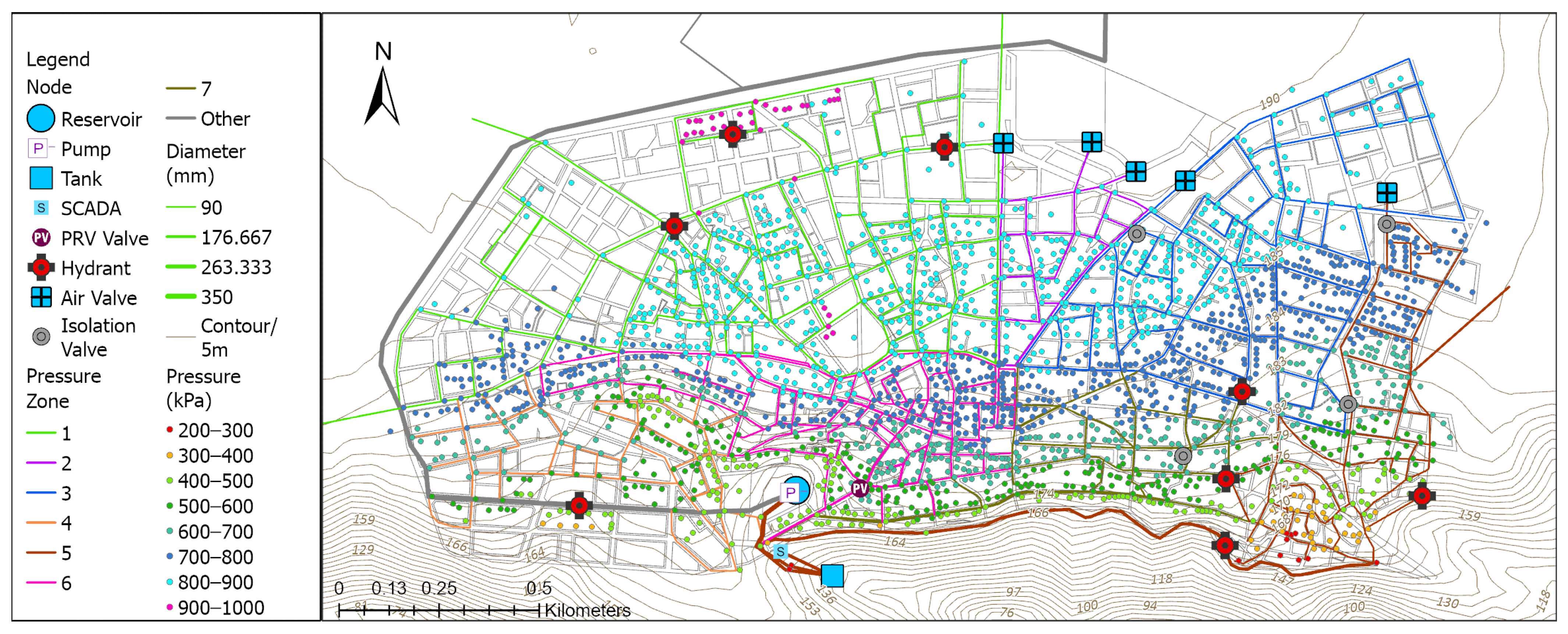
The network is typically designed in a hierarchical order, with an integrated layout of main transmission pipelines that branch into secondary lines. Higher-pressure sources (e.g., reservoirs or pump stations) supply water to areas with lower pressure demands. As water moves further from its source, pressure naturally decreases, so the system is engineered to adjust for this change. Elevation data were analyzed to determine pressure zones (Zone 1, Zone 2, …, Zone 7) and ensure accurate hydraulic modeling. With the aim of controlling the pressures, DMAs were designed and simulated, with the aim of the pressures remaining up to a maximum of 500 kPa, especially in locations with varying elevation or high water demand. DMAs are shown in Figure 4. Within the various pressure zones depicted on the map, PRVs, air valves, and isolation valves help in achieving the specific target pressure range for that zone. For instance, if a zone is defined to operate at 300–400 psi, a PRV or an isolation valve ensures that these zones receive a constant minimum pressure, combating the effects of head loss over long distances. Figure 4 presents the DMAs. The network of pipes is shown as lines, with line thickness indicating the pipe diameter (with a legend indicating classes of ≤90 mm, ≤176.667 mm, ≤263.333 mm, and ≤350 mm pipes).

3.2. Simulation, Hydraulic Model Calibration, and Performance

The simulation starts from the city’s reservoir, which consists of two identical reinforced concrete cisterns at an altitude of 196 m, connected to a pump that draws water from the reservoir, and through the existing conveying pipe, water is sent to the main balancing tank (MBT) located at an altitude of 231 m at the foothills of the mountain, which was designed with a cumulative capacity of 800 m³. From the modeled MBT, through a gravity pipe, the water ends up in the city’s internal aqueduct, where it is distributed to consumers. The simulation presents the operation of the entire water distribution network of the city for 24 h, with data on the level of the MBT from the telemetry, as well as the corresponding supply for 24 h.

The daily demand remained constant at 5500 m³/day for the whole city, but the distribution patterns of water demand were calibrated by trial and error, using the observed data. Peak demand variations are a critical factor in urban water distribution systems. Figure 5 illustrates the fluctuation of the hourly commercial water demand and main supply of the main balancing tank throughout the day. This process went through several stages, with the most important steps being creating appropriate patterns for the total demand throughout the day and specifically approaching the hourly demand. The demand spikes correspond to periods of heightened commercial water use, whereas lower demand is recorded during late-night hours, reflecting minimal network activity, which is typical in densely populated areas.

The graph in Figure 6 presents the performance curve of the city’s reservoir pump. In fact, it illustrates the relationship between the flow rate, the head, and the pump efficiency. As the flow rate increases from 0 to 97.2 L/s, the head (blue line) gradually decreases, indicating a typical pump performance curve. Conversely, pump efficiency (orange line) rises with the flow, reaching a peak ca. 69.4 L/s before declining. This behavior highlights the optimal operating range of the pump, where both head and efficiency are balanced for maximum performance.

Table 4. Hazen-Williams coefficient ranges after calibration.

Pipe Material	Initial Coefficient (C)	Calibrated Coefficient (C)
PVC (majority: 34,731 m)	150	100–120
HDPE (significant: 25,044 m)	155	150–155
Ductile iron (minority: 64 m)	140	130–135

of Hazen–Williams roughness coefficients provides a detailed comparison between the initial values and those adjusted through calibration. The PVC roughness coefficient was significantly reduced from 150 to 100–120, reflecting the aging effects of the pipes and the simulation-confirmed adjustments. This reduction aligns with expected deterioration patterns, where older PVC pipes exhibit increased internal resistance due to material wear, scaling, or minor deformations. The HDPE coefficient remains relatively high (150–155), indicating that its hydraulic performance has not degraded significantly. Ductile iron pipes maintain their expected calibration ranges, ensuring consistency with industry standards and observed network behavior.

Figure 7 illustrates the comparison between the observed and simulated elevation of the MBT. In this 24 h graph, with “continuous red squares”, the real level that emerged from the telemetry system can be distinguished, while the values of the level that emerged from the simulation of the network are marked with the “blue continuous line”.

The hydraulic model was validated using real-time SCADA data and field measurements. The Nash–Sutcliffe efficiency (NSE) of 0.841 demonstrates strong agreement between the observed (x_i) and simulated values (y_i), confirming the model’s reliability for predicting network behavior. According to the established NSE classification ranges [41], values above 0.75 are considered good, above 0.85—very good, which aligns with results from similar studies [4,7,8,12,18], reinforcing the effectiveness of this methodological approach.

The additional metrics, beyond the NSE, provide crucial insights into the model’s robustness and accuracy. A volumetric efficiency (VE) close to 1 (0.9998 in this case) confirms that the model balances input and output volumes accurately, a critical indicator for mass balance in hydraulic networks. The R² value of 0.9002 shows a strong linear correlation between the observed and predicted values. Both mean absolute error (MAE) (0.049) and root mean square error (RMSE) (0.058) are below 0.1, indicating minimal deviation and a close fit between the observed and predicted pressures, consistent with results from [12,29]. Together, these results confirm the model’s robustness, despite the data limitations inherent in the Farsala water distribution system. The validated model can serve as a decision support tool for system optimization, leakage detection, and future network upgrades.

The summary of model calibration performance metrics is presented in

Table 5. Model calibration performance metrics.

Metric	Formula	Range	Benchmark	Value
Nash–Sutcliffe efficiency	$NSE=1-{\displaystyle \frac{{\sum }_{i=1}^n{(x_i-y_i)}^2}{{\sum }_{i=1}^n{(x_i-\overline{x})}^2}}$	(−∞, 1)	≥0.65 (acceptable), ≥0.80 (good), 0.90 (very good)	0.841
Volumetric efficiency	$VE=1-{\displaystyle \frac{{\sum }_{i=1}^n\left|x_i-y_i\right|}{{\sum }_{i=1}^n{x}_i}}$	(0, 1)	Close to 1 (ideal)	0.9998
R2 (coefficient of determination)	$R^2={\left[{\displaystyle \frac{{\sum }_{i=1}^n(x_i-\overline{x})(y_i-\overline{y})}{\sqrt{{\sum }_{i=1}^n{(x_i-\overline{x})}^2}\times \sqrt{{\sum }_{i=1}^n{(y_i-\overline{y})}^2}}}\right]}^2$	(0, 1)	>0.85 (strong fit)	0.9002
MAE (mean absolute error)	$MAE={\displaystyle \frac{{\sum }_{i=1}^n\left|x_i-y_i\right|}{n}}$	(0, +∞)	Ideal > RMSE	0.049
RMSE (root mean square error)	$RMSE=\sqrt{{\displaystyle \frac{1}{n}}{\sum }_{i=1}^n{(x_i-y_i)}^2}$	(0, +∞)	<0.1 (good fit)	0.058

. This table provides a detailed overview of each evaluation metric, including its mathematical formulation, typical value ranges, accepted benchmarks, and the corresponding values obtained in this study. Formulas for each metric are derived from standard hydrological and statistical modeling references, including [40] for NSE, [43] for MAE and RMSE, and established statistical principles for R² and SE. The benchmarks follow common practices for water distribution system modeling (e.g., [12,29]).

3.3. Extended Period Simulation (EPS) Analysis

EPS were conducted over a 24 h cycle, analyzing demand fluctuations. The EPS was set with a 10 min step interval and a 24 h simulation duration based on SCADA telemetry data. Reservoir levels and pump operation patterns were analyzed to assess system efficiency. Peak demand periods resulted in pressure drops of 3% (11 kPa), while off-peak hours allowed for system recovery.

Table 6. Reservoir, tank, and pump performance.

Time of Day	Reservoir/Pump Head (m)	Pump Flow Rate (L/s)	Tank Head (m)	Efficiency (%)	Pressure Drop
00:00	39.1	87.5	39.1	48.9	–0.1%
06:00	39.2	87.5	39.1	48.9	–0.3%
12:00	39.9	87.3	38.8	49.9	–2.8%
18:00	40	87.3	39.1	50	–2.2%
24:00	38.7	87.6	38.7	48.4	0.1%

presents the reservoir, tank, and pump performance.

Figure 8 presents pressure variation over the network. Service nodes are colored to show pressure zones, indicated by a color gradient from red (200–300 kPa) to magenta (900–1000 kPa), showing the pressure at different points throughout the network. The pressures of the network along its entire length are characterized as very high, exceeding 9 atm. The highest pressures are found in the flattest areas of the city to the north, where most of the network damages occur, due to the significantly elevated static pressures and the lack of pressure regulation infrastructure such as PRVs and isolation valves.

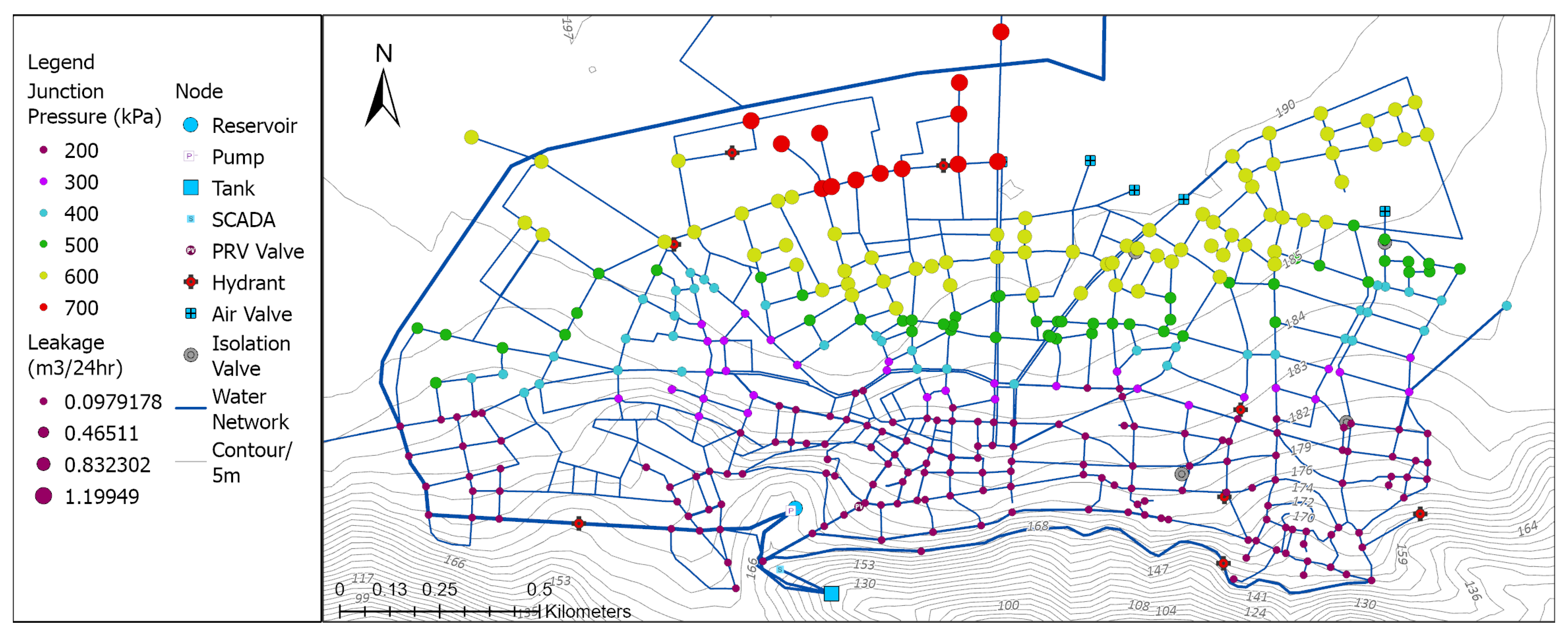
Leakage detection simulations identified high loss areas. Figure 9 presents junction pressures and leakage rates. Junctions are colored circles representing different pressures (200–700 kPa) and sizes depending on the amount of leakage (0.098–1.2 m³/24 h). The total leakage is estimated at 10–20 m³/24 h, depending on the number of junctions with each level of leakage. Specific junction pressures vary widely and are indicated by the color of the node. The analysis of leakage hotspots indicates that leakages are pressure-induced, and occur in the flattest areas of the network, aligning with pressure distribution patterns.

4. Discussion

This study presents a comprehensive hydraulic modeling framework for the water distribution network of the city of Farsala, integrating CAD-based digitization, GIS spatial data, and real-time SCADA telemetry under conditions of significant data scarcity. The novelty of the work lies in the methodology’s adaptability to incomplete or outdated datasets, demonstrating that a reliable and operationally useful model can still be developed when traditional records and infrastructure documentation are lacking. By synthesizing digital mapping, geospatial analysis, and telemetry-informed calibration, this study sets a precedent for under-resourced utilities, echoing the findings of [24] on the utility of virtual modeling platforms to digitize previously unmapped networks. Similar challenges are identified in [23], which highlighted the limitations in data availability for small municipalities and proposed integrated modeling approaches under constrained conditions.

The modeling process, anchored in AutoCAD digitization and enhanced with GIS elevation data and satellite imagery, allowed for the first complete mapping of Farsala’s network since its initial construction. The identification and georeferencing of the key infrastructure components, such as pressure pipes, laterals, tanks, hydrants, and valves, produced a high-fidelity spatial model that both improved visualization and served as the basis for hydraulic simulation. These practices align with recommendations by Grison [2,25] regarding GIS-based data integration for smart water infrastructure.

The performance metrics obtained in this study, with Nash–Sutcliffe efficiency (NSE) of 0.841, volumetric efficiency of 0.9998, R² of 0.9002, MAE of 0.049, and RMSE of 0.058, demonstrate the model’s high accuracy in replicating the real-world behavior of the Farsala water distribution system. When compared to the results of [12], which reported an NSE of 0.82 in simulations of leakage dynamics, and [29], which obtained an NSE of 0.85 in calibrating potable water networks using WaterGEMS and SCADA data, the performance of this study was comparable and within the upper range of acceptable accuracy thresholds. Similar values were also reported in [8], where Bayesian calibration incorporating historical demand data yielded NSE values exceeding 0.80, further validating that such levels of accuracy are indicative of reliable hydraulic models. Therefore, the results of this study fall well within the range of accepted values for urban water distribution system simulations and confirm that even under significant data limitations, it is possible to develop robust and reliable hydraulic models.

The zoning of the network into seven pressure areas and the introduction of DMAs based on elevation and demand patterns reflect the current best practices in pressure management and demand allocation, as also discussed in [7,8], which emphasized the importance of demand pattern calibration in water resource planning. The critical modeling decision to simulate the system beginning from the reservoir rather than from boreholes helped overcome the well-known limitations of groundwater abstraction modeling in WaterGEMS, a challenge similarly noted in [4,18].

Despite these strengths, the results also reveal significant systemic weaknesses. The network operates at consistently high pressures (>900 kPa in many zones), exceeding the standard design limits and increasing the risk of pipe failures, leakage, and customer-side damage, an issue reinforced in [10] in relation to critical pipe identification, and in [36] in relation to pressure-induced leakage dynamics. The analysis of leakage hotspots further validates this concern, identifying flow losses of up to 1.2 m³/day at individual junctions, particularly in high-pressure or older pipe segments, consistent with patterns observed in [11], which used SCADA-informed pressure simulations to detect similar anomalies.

The spatial layout also reveals a dense core distribution zone that transitions into sparsely connected peripheral areas, typical of towns experiencing urban expansion without coordinated infrastructure updates, as noted in [28]. The placement of control elements, which is currently limited to a single PRV, four isolation valves, and one SCADA monitoring point, is clearly inadequate for managing dynamic flow conditions and pressure variability across a geographically diverse area. This is in contrast to more advanced configurations recommended in [21] for real-time control and in [17] for efficient EPANET-driven simulations. Strategic expansion of these elements, guided by model outputs, could significantly enhance resilience and reduce non-revenue water (NRW), a challenge extensively discussed in [9,12].

Importantly, this model demonstrates how SCADA data, even when limited, can be used not only for monitoring but also for model calibration and validation, bridging the gap between theoretical simulation and operational reality. The integration of EPS analysis further highlights daily fluctuations in demand and pressure, providing operational insights similar to those explored in [6], validating the model’s temporal accuracy, and pointing to time windows of operational stress.

Together, these contributions position the Farsala model as a practical reference for other small cities facing similar challenges in water network modernization under data-limited conditions.

5. Conclusions

This study developed a comprehensive hydraulic modeling framework for the Farsala water distribution network, integrating AutoCAD digitization, GIS-based spatial analysis, and SCADA-driven real-time telemetry, despite significant data constraints. The methodology produced the first high-resolution digital representation of the city’s water infrastructure, enhancing system visualization, operational decision-making, and long-term planning. The model’s validation metrics confirm its accuracy in simulating network behavior. Additionally, EPS identified peak demand fluctuations, pressure variations, and critical infrastructure vulnerabilities, providing actionable insights for municipal planning.

However, several challenges remain in the hydraulic modeling of Farsala’s network. The limited availability of historical records necessitated data interpolation, introducing potential uncertainties in model predictions. High-pressure zones exceeding 900 kPa were identified as critical leakage hotspots, increasing the risk of pipe failures and distribution inefficiencies. The lack of sufficient control elements, such as pressure regulation valves (PRVs) and isolation valves, continues to exacerbate pressure imbalances, limiting operational flexibility. Additionally, the relatively recent implementation of SCADA telemetry provided constrained input data, restricting full-scale validation of transient network behavior. Furthermore, the absence of historical records on pipeline materials and valve locations complicates maintenance strategies and emergency response planning.

Despite these limitations, the methodology presents a scalable solution for municipalities facing data scarcity and aging infrastructure challenges. It enables enhanced operational control, leakage reduction, and strategic rehabilitation planning, supporting modernization efforts in water distribution management.

Future research should explore integrating predictive leakage management using machine learning, expanding SCADA functionalities for real-time adaptive control, and optimizing energy efficiency through dynamic pump scheduling. Additionally, incorporating climate-responsive infrastructure planning will improve system resilience against extreme weather conditions. Advancing IoT integration and smart city technologies could further strengthen transparency, automation, and responsiveness in urban water management.

These advancements position the model as a valuable decision support tool for municipalities seeking scalable, data-driven solutions for infrastructure modernization and sustainability.