Detection of Cracks in Arch Dams Using Monitoring Data and Numerical Models

Abstract

A methodology based on displacement measurements from monitoring devices is proposed and tested. The goal is to detect the formation of cracks in arch dams and estimate their dimensions using a straightforward approach. The methodology involves interpolating displacement data against representative cases to identify anomalies indicative of cracks. A real dam was used as a case study, which began with the development of a 3D finite element model under several hypotheses. This model was analyzed using finite element method (FEM) calculations to simulate the displacements recorded by monitoring devices. The effectiveness of the methodology was evaluated based on the number and location of monitoring stations, demonstrating its ability to detect cracks and approximate their dimensions with acceptable accuracy.

1. Introduction

1.1. Dam Safety

During the early 20th century, particularly, a significant development of hydropower began in many developed countries, leading to the construction of numerous dams. For the most part, these dams remain in operation, and, although aged, they are expected to remain operational for many years. Looking specifically at high arch dams, it can be seen that most of them suffered unexpected cracks during the construction stage or in service operation [1,2,3,4] and therefore, it is important to evaluate the structural safety of these dams [5].

Providing safe and reliable operation of dams throughout their service life is a major interest all over the world. To this end, the significance of monitoring and analyzing the behavior of large concrete dams, especially by using experimental data along with numerical modeling, has been well recognized for decades [6,7]. Hence, it is a major concern to provide accurate analysis methods to evaluate the present condition of dams as well as to assess the safety of these structures, especially the partially damaged ones. However, due to the inherent complexity of the dam foundation system, no method is available nowadays that automatically detects the cracks in an arch dam based on monitoring data.

1.2. Crack Detection

The majority of newly constructed and rehabilitated dams have structural health monitoring (SHM) systems that provide real-time screening and monitoring of the safety and health condition of the structures [8,9]. An adequate evaluation of the aging of dams provides a better understanding of their present safety as well as enabling better planning of rehabilitation and reconstruction investments. Therefore, the monitoring of dams plays a key role in dam safety operations and has become indispensable for the identification of behavioral changes that may develop over the lifetime of the dams.

The prediction of measurements and the interpretation of the behavior of dams, using the data obtained from the measurements, is a standard practice nowadays for dam engineers [10,11,12]. In this regard, the use of different forms of behavioral models (digital twins) makes a major contribution in capturing the performance of a dam, making such behavioral models a key component of dam safety systems.

Nowadays, engineers can use predictive models to evaluate dam behavior, estimate dam response to actual loading conditions, and establish warning levels. Both data-driven models and numerical models based on the finite element method (FEM) have been extensively applied to predict dam displacements, stresses, and strains and, thereby, to estimate the response of the dam [10,11,13]. As computing power has increased, both data-driven and numerical models have improved in terms of their level of detail and precision, as well as their complexity.

In this work, a methodology using FEM models was developed based on the displacements measured in the monitoring devices of an arch dam. This methodology aims to detect if a crack has been formed in the dam and, as a second goal, to estimate the severity of this crack. For this purpose, the results of the monitoring devices were compared with the simulated movements based on certain reference cracks.

As a first step, it was necessary to create a 3D model of the dam to be analyzed; in this sense, the tests of the methodology were carried out on a real dam by adding several reference cracks. Later, this 3D model will be used to calculate the displacements through FEM simulations, as if they were measured in the monitoring devices.

2. Methods

2.1. General Approach

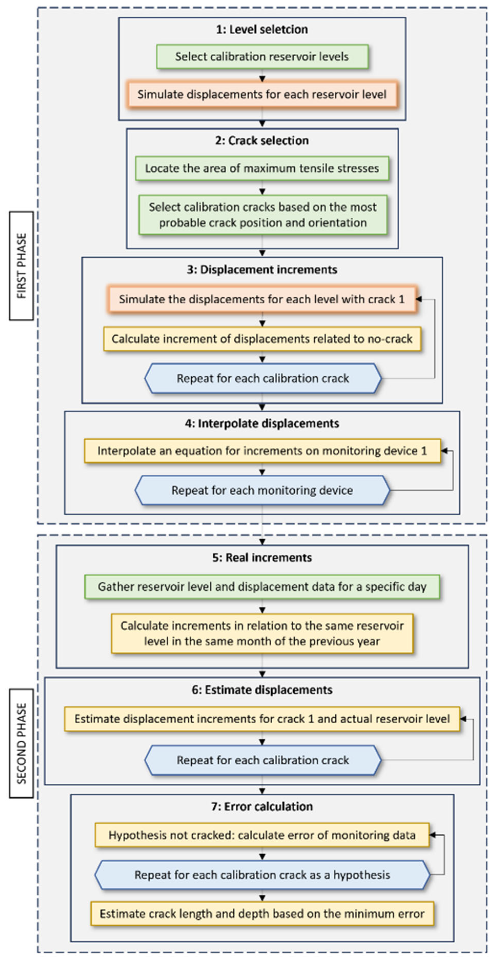
The proposed method for crack detection (Figure 1) applies to any specific dam with known geometry, material properties, and records of monitoring devices and reservoir level (current and from a previous year). For real cases, the first phase of the methodology is performed before analyzing current dam records and involves four steps. Step 1: Select calibration reservoir levels and simulate, for each one, the displacements at the monitoring points. Step 2: Locate the area where cracks are most likely to appear based on tensile stresses, determine (by expert judgment) the most probable crack shape, and select calibration cracks. Step 3: Simulate, for each crack and reservoir level, the displacements at the monitoring points and calculate their difference against the displacement without any crack. Step 4: For each calibration crack and each monitoring device, determine an equation indicating the incremental value for any given reservoir level, based on the interpolation of the simulated levels. Steps 2 and 3 may be repeated as many times as desired in order to have a good collection of possible cases from which to interpolate. This whole process, which requires computation resources, is only performed once and may be used throughout the life of the dam.

The second phase takes place when data from a specific time of the dam is to be analyzed. This phase consists of three more steps. Step 5: Gather the current reservoir level and displacement data and calculate increments in relation to the dam without cracks, assumed as the same reservoir level in the same month of the previous year. Step 6: Estimate, in accordance with the equations of step 4, for each calibration crack, the displacement increments under the actual reservoir level by interpolating the increments of the representative reservoir levels. Step 7: Under the hypothesis that the dam was not cracked, calculate the error of the real data, then re-calculate, changing the hypothesis to each calibration crack. Finally, the minimum error is interpolated to estimate the real crack dimensions.

An alternative methodology will be analyzed under the variation that step 4 is omitted and that in step 6, new FEM simulations are performed for each calibration crack with the current reservoir level. This methodology requires more calculation time each time an actual situation is to be monitored; therefore, it is not suitable for continuous monitoring systems. The article focuses on whether these methodologies are valid for detecting cracks or not, compared with the precision of the monitoring devices, rather than on how accurate these are simulated.

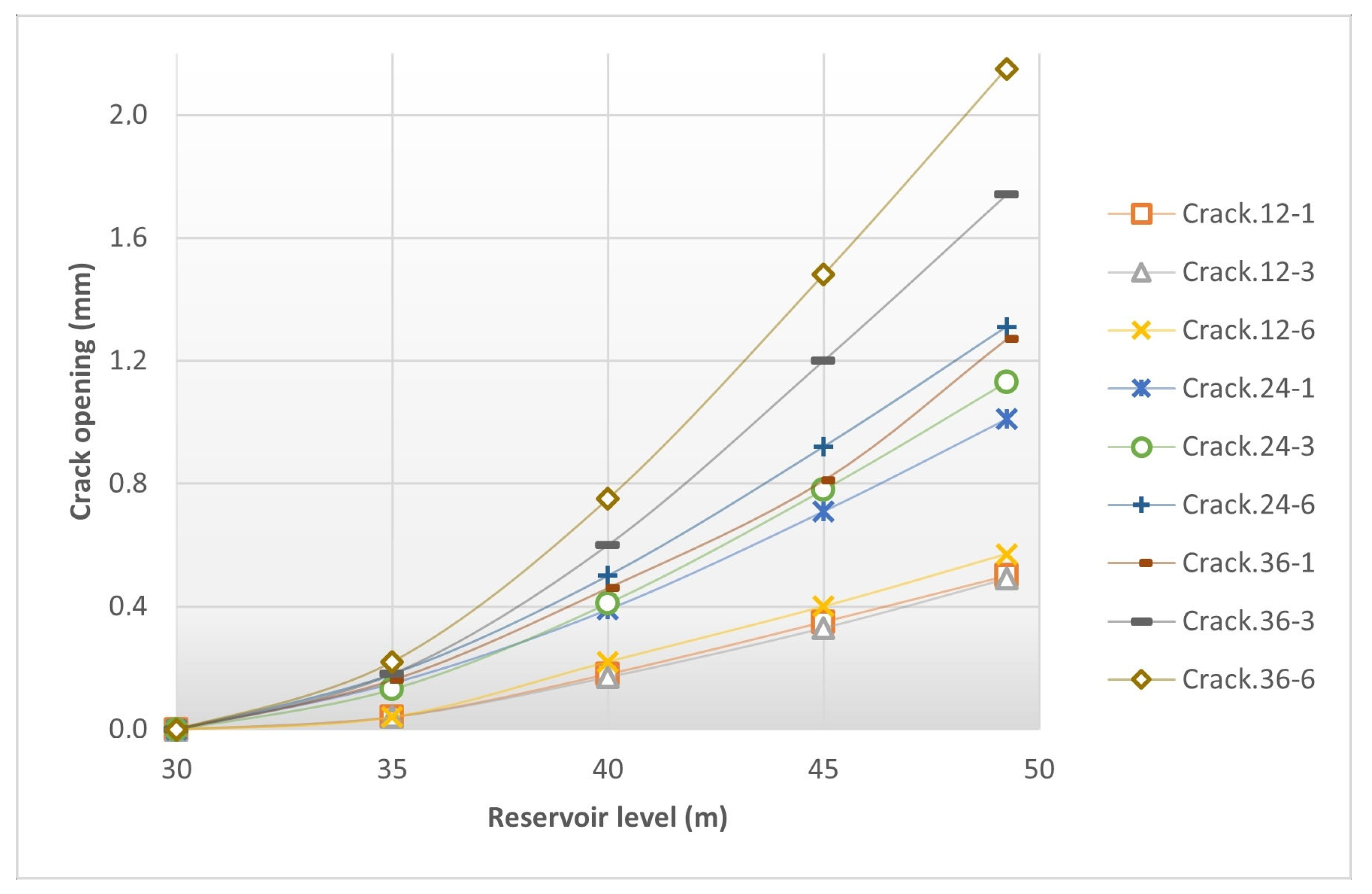
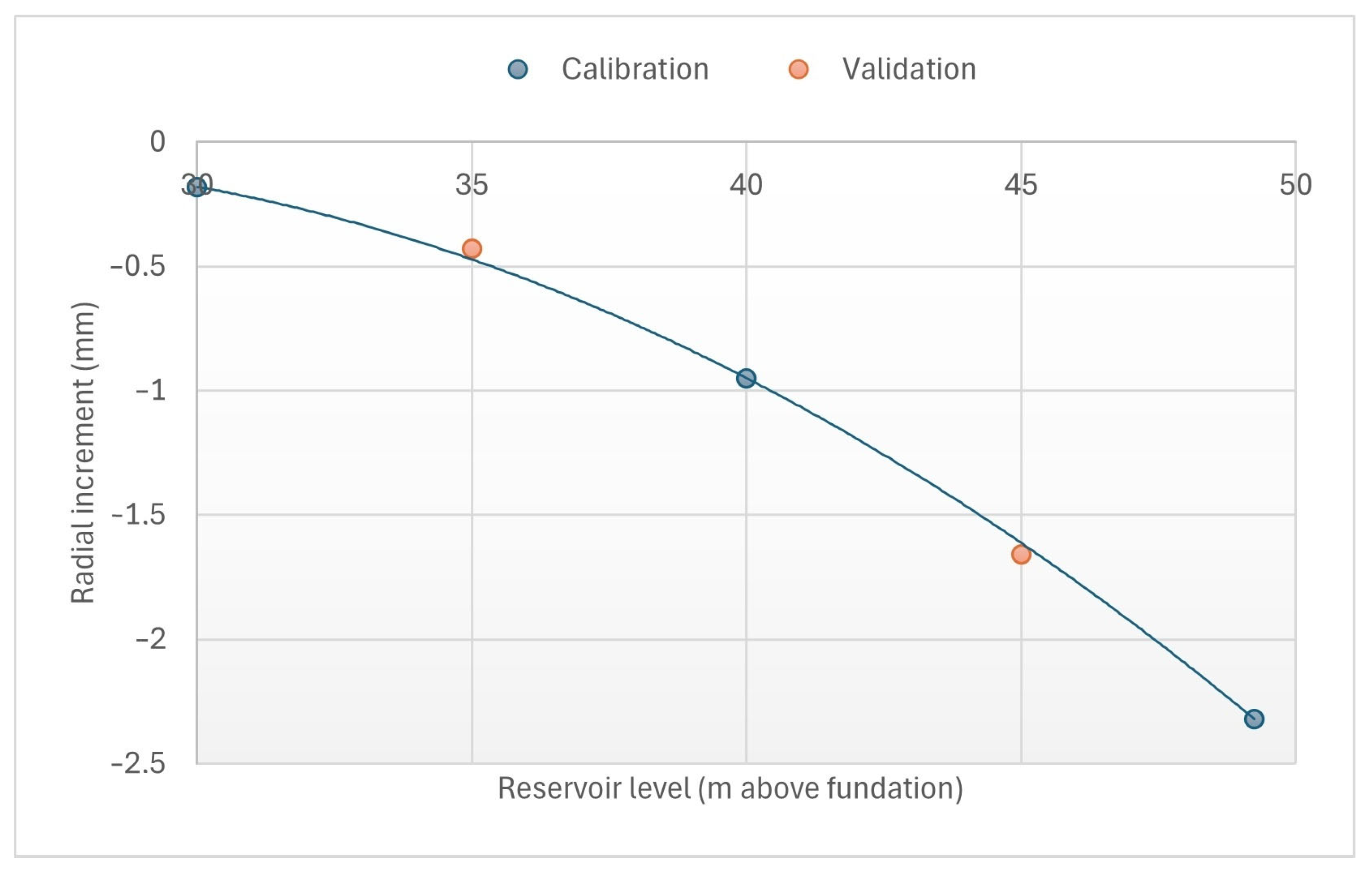
Throughout this paper, a numerical experimentation campaign on a case study was performed to test these methodologies for the detection of cracks in arch dams. It should be clarified that it was decided to use three calibration reservoir levels, although the method would be valid for any number of levels. To verify that the methodologies work properly, nine calibration cracks and four validation cracks were simulated, allowing the number of cases in which the identification works correctly to be tested.

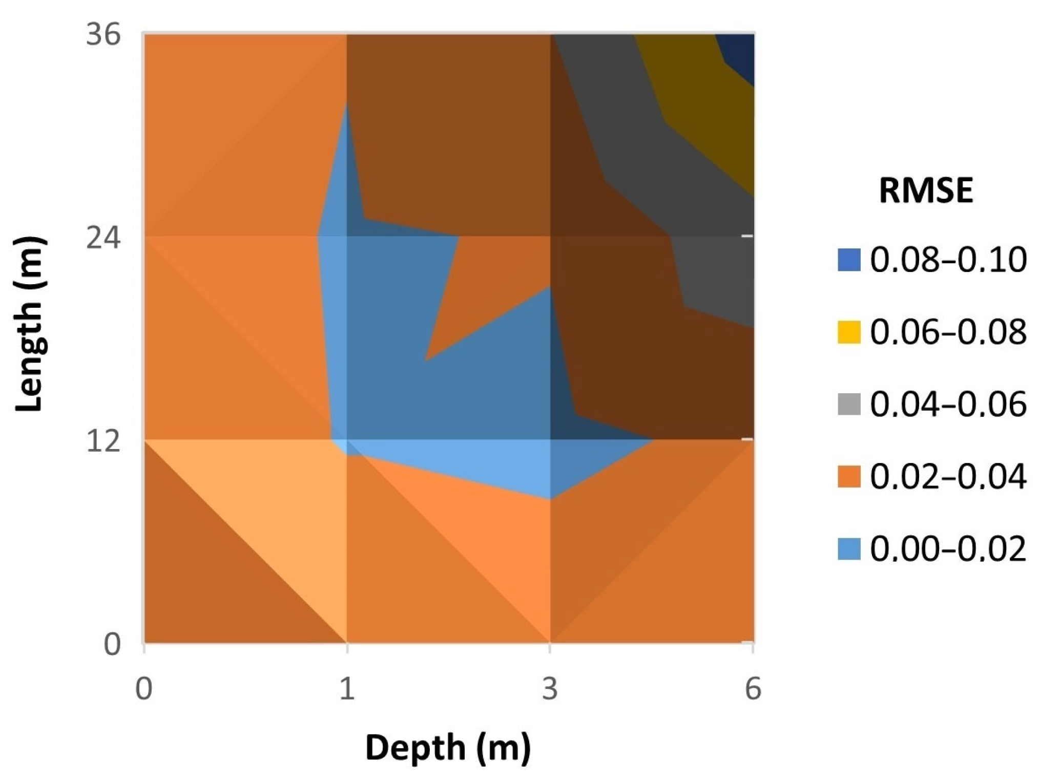
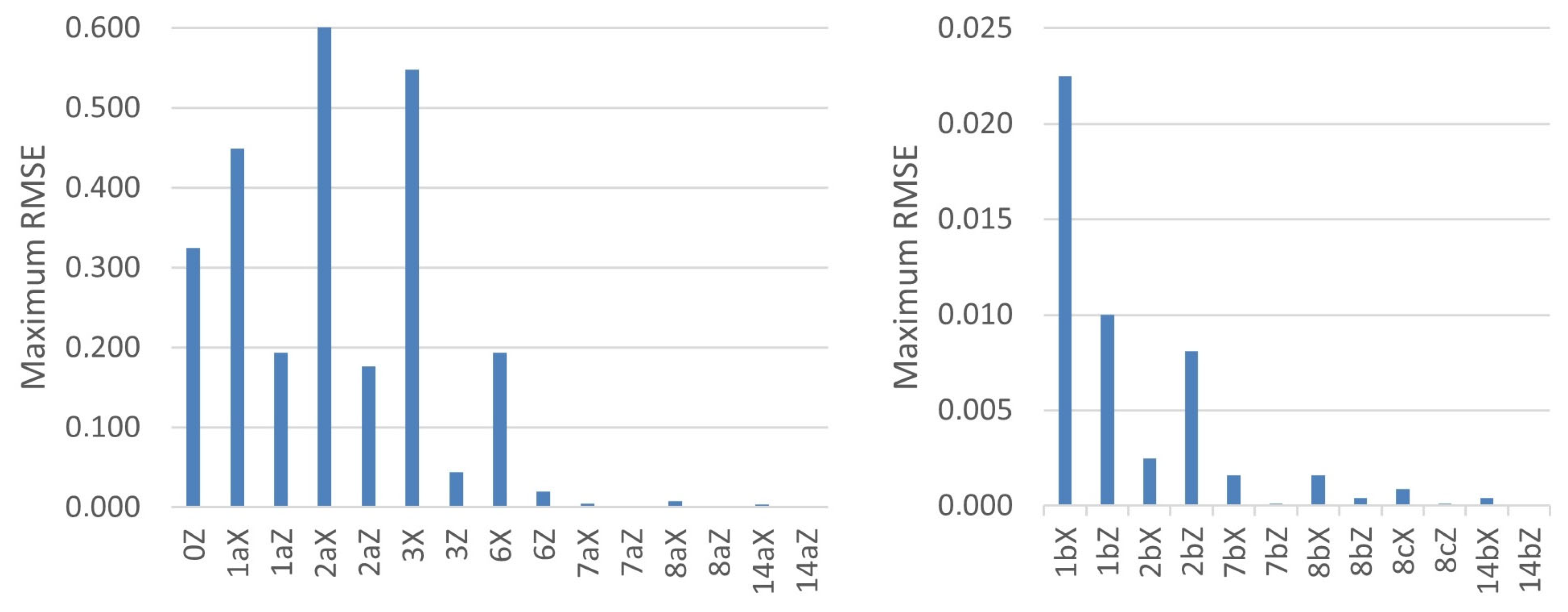
To calculate errors, the results were contrasted using two measures. The first was a plain Mean Absolute Error (MAE) while the second was the Root Mean Squared Error (RMSE). RMSE was included because it increases the importance of large errors and reduces the importance of small errors, which may be due to measurement inaccuracy. Relative error measures were not used in this study because, at points where the displacement is quite low, the measurement uncertainty can lead to exceedingly high relative errors.

$$RMSE=\sqrt{{\displaystyle \frac{1}{N}}{\displaystyle \sum }_{i=1}^N{\left(x_i-y_i\right)}^2}$$

(1)

(1) Here, x—calculated value; y—expected value; and N—number of monitoring points.

2.2. Numerical Approach

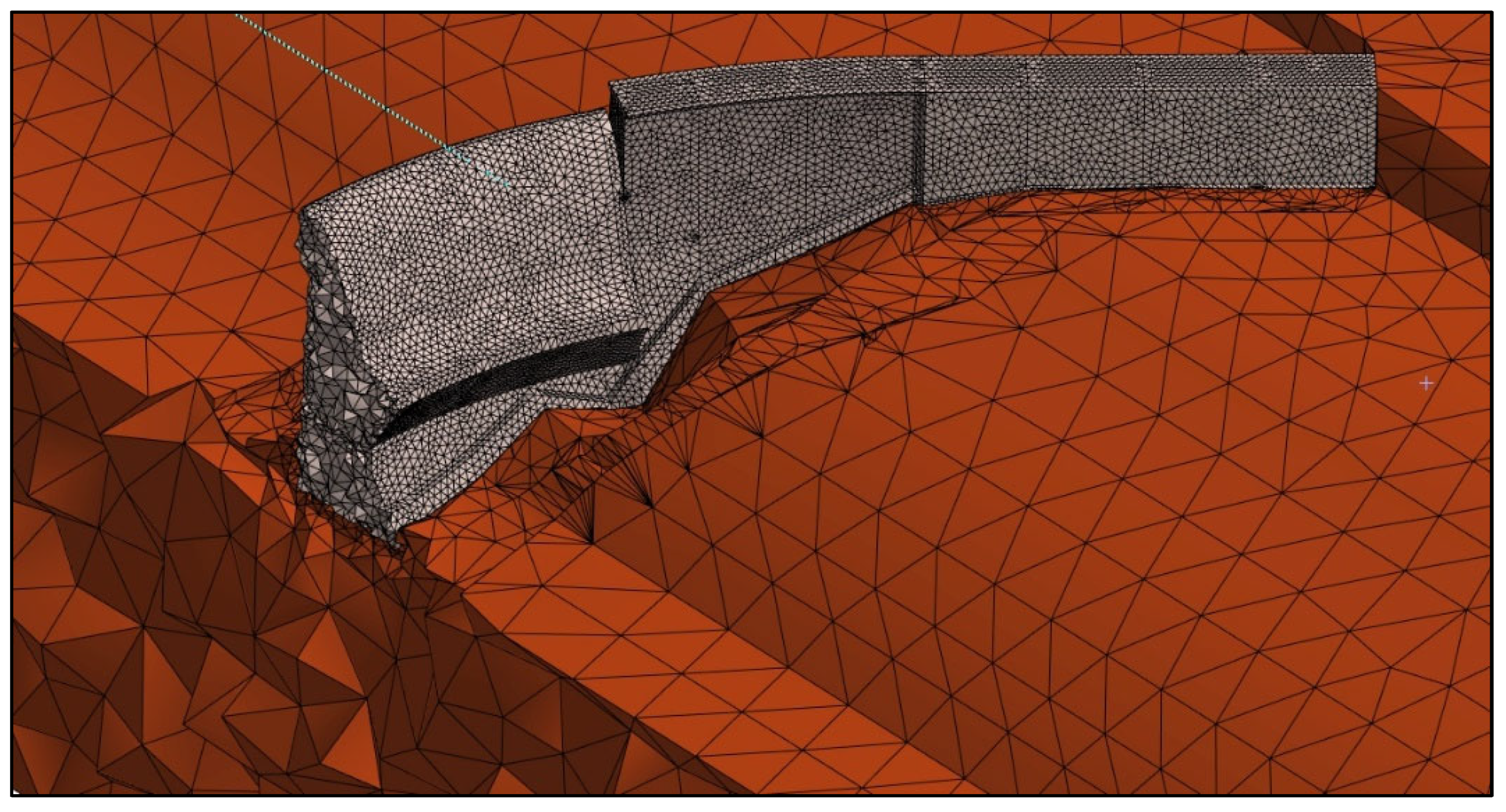
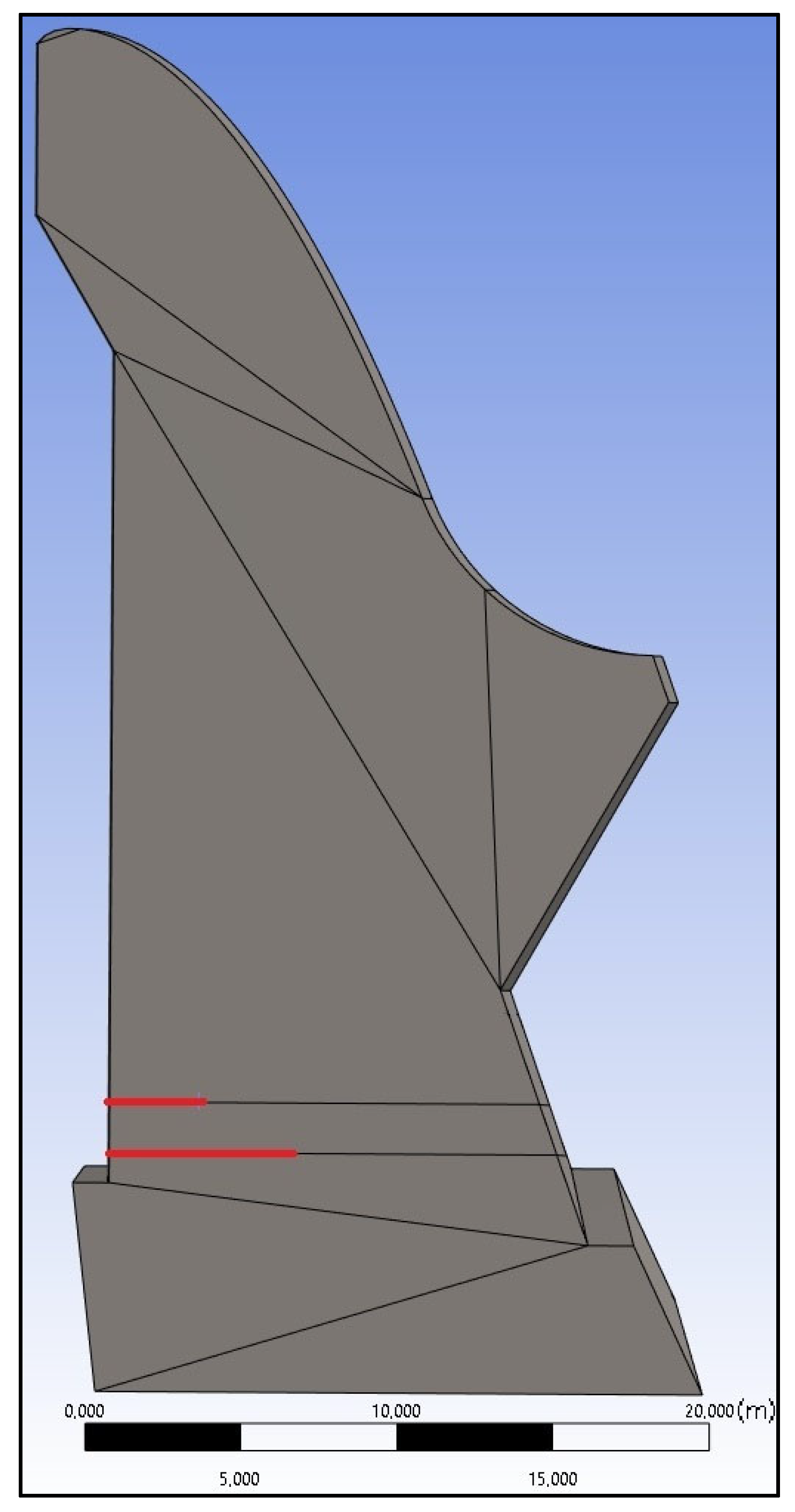
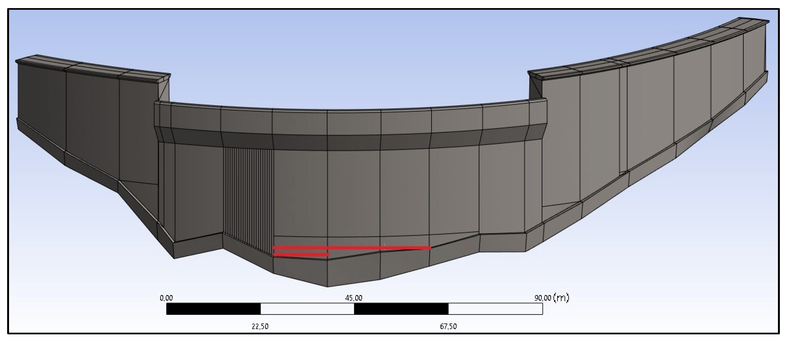
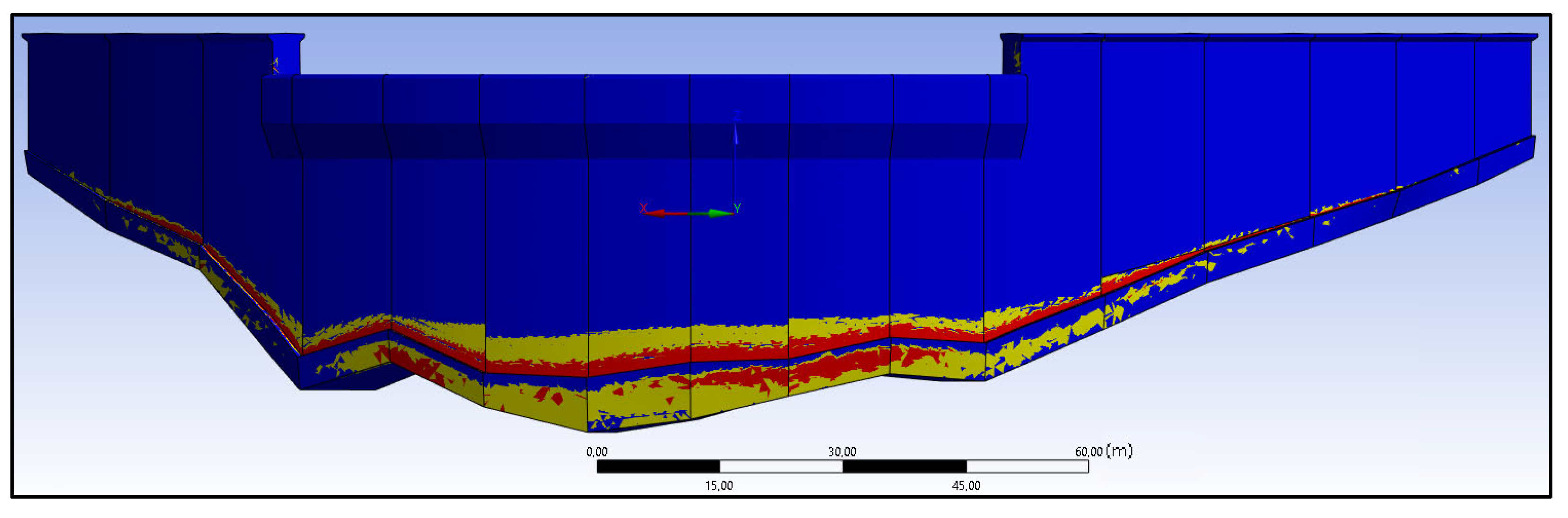
The core work of this study consisted of a campaign of numerical simulations based on the finite element method (FEM) to measure displacements in a real dam when subjected to a crack of variable length and depth. Once the displacements are calculated, the records that would be obtained by monitoring devices at different points of the dam are determined to analyze whether they can detect the size of the cracks.

To perform all the numerical simulations of the dam foundation system contemplated in this work, the Ansys Mechanical Finite Element Analysis Software for Structural Engineering 2022 [14] was employed, along with 3D models. In the calculations involving friction surfaces, the iterative Preconditioned Conjugate Gradient solver was used with a tolerance value of 10⁻⁸, a maximum number of substeps equal to 4, and a maximum number of iterations equal to the number of nodes times the degrees of freedom of each node. The numerical model adopted presented the following features: (a) linear materials (stress–strain curve); (b) static models; (c) no separation between the dam and the ground; (d) nonlinear contacts (cracks).

The self-weight of the dam, the thermal stress, and the hydrostatic pressure of the reservoir in the upstream part of the dam and the internal sides of the crack were the only active forces. The nonlinearity of the materials has not been considered since it makes no direct impact on the deformations of the dam after cracking, which is the purpose of this work. Instrumentation devices were used to capture the movement in a small range of years, for which concrete properties are considered constant.

Since the main objective of this work was to analyze cases of dangerous cracking, it was necessary to consider cracks that open up enough to significantly affect the behavioral response of the dam. Therefore, it was of interest to study situations where dam conditions favor the opening of significant cracks; however, dams are specifically engineered to avoid crack opening under the usual loads they would normally bear.

In addition to hydrostatic pressure and temperature variations, other causes can favor or reduce the opening of cracks in the dam: heterogeneity of concrete properties, concrete aging, expansive chemical reactions, shrinkage, alkali–aggregate reactions, microseismicity, foundation deformation, seepage, inadequate design or execution of construction and maintenance, freeze–thaw effects, or hydration heat during concrete curing. Simulating all these conditions in a general approach with the purpose of finding the most unfavorable cases for the creation of cracks would require an unaffordable amount of calculation time. For a specific dam, some of these conditions may need to be simulated. A previous analysis of the dam (history, behavior, etc.) will lead to the conclusion of which aspects to be considered in the analysis.

As this study is interested in the cases that can favor the opening of cracks in the dam, the uncertainty in the results caused by not considering the rest of the forces is assumed to be smaller than the effect of including a large thermal effect. It is important to clarify that the objective of this work was not to achieve an extremely realistic stress distribution but rather to analyze the capacity of a monitoring device to identify a crack in the dam.

For the analysis of the cracking effect, the presence of a significant crack in the dam was assumed; therefore, the mesh was designed to align the faces of the elements with the sides of the crack. These cracks were considered fully formed, so the development process was not considered. Cases in which two relevant cracks open simultaneously or in which cracking develops at the same time as one of the transverse joints opens are very rare, so these cases were not included in the study.

The methodology applied for numerical simulations takes into account that the dam structure is changed before the development of hydrostatic pressures, but after self-weight has already taken effect, by sealing the transverse joints and, therefore, binding the individual blocks together into a monolithic structure. It was also considered that, after joint sealing, the dam changes again to a third configuration at the moment a crack emerges. Consequently, at the first stage, when self-weight is the only load, the sides of the joints can propagate compressive or frictional forces while moving independently, as long as they do not intersect each other, following their actual behavior. On the contrary, in the second and final stages, the dam joints react in a monolithic way. Therefore, the sides of the same joint are deformed as one, while always keeping the same relative position they showed at the end of the self-weighing phase. This study builds on a theoretical model, based on the actual geometry of a dam, to which several simplifications have been made to limit the number of possible variables, thereby making direct evaluation with the real dam measurements no longer applicable; however, the model was previously validated in [15], where the geometry and properties of the dam belong to the same type.

The boundary conditions applied in the numerical models correspond to those common for this type of simulation: constrain the horizontal movements on the sides of the soil body and constrain any movement at the lower base of the soil. The extent of ground included in the 3D model on each side of the structure was the conventional dimensions for structural analyses [16], so that the applied boundary conditions do not alter the obtained results. Specifically, it was completed with terrain horizontally up to 50% of the length of the dam on the left and right sides, while the depth, upstream, and downstream directions of the terrain extend 150% of the height of the dam.

2.3. Study Case

2.3.1. Dam, Foundation, and Loads

A real concrete arch dam with a height of 50.25 m and a crest length of 535.3 m was used as a model. The foundation was composed of igneous rocks, mainly granodiorites and dacites. Based on existing studies of this dam and due to the lack of more precise available data, the simplification that the foundation material is homogeneous was assumed and, consequently, the bedrock can be simplified to average values of the bedrock properties. As field borings do not analyze Poisson’s modulus, an average value corresponding to that type of rock was assumed. The influence of variations in the Poisson’s value on dam movements is demonstrated in the literature to be very low [17]. Likewise, in the absence of specific studies of the concrete of the dam, a concrete–concrete rough interface friction coefficient for dry conditions of 0.8 was assumed for concrete grades ≤ C50/60. All other material properties were obtained from the dam reports (

Table 1. Material properties.

Material	Foundation	Concrete
Density (kg/m3)	2620	2350
Modulus of elasticity (MPa)	51,500	19,600
Poisson’s ratio	0.165 [18]	0.2
Coefficient of Thermal Expansion (°C−1)	8.43 × 10−6 [19]	10−5 [20]
Friction coefficient	-	0.8 [20,21,22]

).

Three reservoir levels were considered for the numerical model calibration: 49.24 m above foundation (Extreme Flood Level), 40 m, and 30 m. In addition, another two reservoir levels were considered to validate the performance of the method: 45 m (Maximum Normal Level) and 35 m. Lower levels were not simulated, taking into consideration that the upstream cracks do not open, and the behavior of the dam is almost identical to that of a non-cracked dam when the hydrostatic pressure is low.

As this is an exploratory study aimed at evaluating the potential of the methodology, the objective is to see if the order of magnitude obtained falls within the range of what can be captured by the monitoring device. As this is the core objective, the study should not be made overly complex in order to achieve unnecessary precision. Therefore, it was assumed that the effect of a homogeneous thermal decrease on dam displacement is similar to the non-homogeneous decrease with the same mean value. Although the displacements of the dam will not be the real ones, they remain very close to the actual displacements. Therefore, the thermal stress condition consisted of a theoretical uniform temperature drop over the entire dam of 5 °C in relation to the temperature at the time of joint grouting. It was expected that an approximately linear relationship between the temperature increase and the crack opening (as verified in Section 3.1) would be found; therefore, the results for any temperature value can be estimated from the results obtained for a 5 °C drop.

2.3.2. Monitoring Devices

This paper analyzed the synthetic results of radial and vertical displacements modeled numerically. Circumferential displacements were not discussed, given that such displacements do not play a significant role in the behavior of a cracked arch dam.

Displacements are recorded at 19 points (

Table 2. Displacement monitoring devices at the dam.

Block	Monitoring Device	X (m.)	Y (m.)	Z (m.)	Elevation Above Foundation (m.)
0	Leveling screw P5	146.2	83.1	79.0	39.8
1	Pendulum PI-B1-GH	164.8	79.3	58.3	18.3
1	Pendulum PI-B1-GP	164.8	79.3	45.0	5.0
2	Pendulum PI-B2-GH	133.8	83.0	60.2	18.9
2	Pendulum PI-B2-GP	133.8	83.0	45.3	4.0
3	Leveling screw P6	174.2	75.5	79.0	34.7
6	Leveling screw P4	117.2	81.7	79.0	33.9
7	Leveling screw P7	196.9	62.1	87.0	36.2
7	Pendulum PI-B7-GP	196.1	63.8	63.9	13.1
8	Leveling screw P3	96.0	75.0	87.0	39.5
8	Pendulum PI-B8-GH	103.8	76.8	61.7	14.2
8	Pendulum PI-B8-GP	103.8	76.8	53.1	5.6
14	Leveling screw P2	62.2	50.3	87.0	24.3
14	Pendulum PI-B14-GP	64.1	50.6	67.7	5.0

) corresponding to the location of the installed monitoring devices. Among them, the five points corresponding to direct pendulums are located at short distances from the monitoring points of inverse pendulums. Two monitoring points at close distance do not provide useful information; therefore, direct pendulums were not considered.

The studied monitoring points were increased to include at least two points per block (Figure 2). These additional monitoring points were placed at the crest of the dam or at an average height, selecting as the average height that of the pendulum PI-B7-GP.

2.3.3. Three-Dimensional Geometric Characterization and Mesh

The 3D design was based on the topography records and cross sections of the dam (Figure 3). The model was simplified by eliminating galleries, bottom drainage, crest railings, stairs, and the board over the spillway.

Figure 4 shows the dam ground plan, which consists of 3 arches with 2 different curvatures, covering 16 blocks, and abutments at each end in straight alignment, covering another 6 blocks.

The ground not immediately adjacent to the dam was simplified, while detailed ground definition, with contour lines every meter, was included adjacent to the dam.

Tetrahedra with 10 nodes were used for the mesh, and a quadratic element order and a growth ratio of 1.1 (Figure 5). The rest of the parameters were established to maintain a compromise between the calculation time and the quality of the result. All the mesh features have been extracted from a mesh convergence study previously tested in similar cases under the same numerical model [15]. The mesh has 462.570 elements and 713.295 nodes, based on maximum mesh sizes of 1.12 m for the dam and 11.2 m for the bedrock, which were considered optimum in a similar case [15].

2.3.4. Cracks

To determine the most probable cracking zone for this dam, a preliminary test was carried out as explained in Section 3.1. In that area (upstream, center, close to the base), different cracks were considered with lengths and depths of relevant significance to ensure a clearly visible effect on the deformation of the structure.

To consider the different types of probable cracking, nine cracks were defined with depths of 1, 3, and 6 m (Figure 6) and lengths of 12, 24, and 36 m (Figure 7). Cracks always start and end at a block joint and are located along blocks 0, 1, and 2. Cracks 12 m long are located in block 1, and those 24 m long span blocks 0 and 1. In addition, four other cracks, namely A, B, C, and D, were used for validation: 2 and 4.5 m deep; 15 and 21 m long.

3. Results

The main objective of the study was to test the methodology for detecting and estimating cracks based on the simulated displacements that might have been recorded by monitoring devices.

3.1. Preliminary Analysis

To locate the most probable cracking zone, a case of reservoir level equal to the Maximum Normal Level and zero thermal stress was calculated, proving that the zone with tension greater than 0.2 MPa was located mainly at the base of the upstream face of the central blocks (Figure 8).

Once the models for the nine cracks were created, the dam behavior for five reservoir levels was simulated, showing that the crack opened in all cases for levels greater than 30 m above the foundation (Figure 9).

To verify the accuracy of estimating displacement results, the simulations for all cracks with reservoir levels of 35 and 45 m were compared against interpolation equations based on the other simulations (Figure 10 shows one example). These interpolations were performed using parabolic equations based on simulations for 30, 40, and 49.24 reservoir levels. It was concluded that the error in the displacements was found to be acceptable (

Table 3. Interpolation mean errors.

	35 m Above Foundation		45 m Above Foundation
	MAE	RMSE	MAE	RMSE
Crack 12-1	0.003 mm	0.005 mm	0.003 mm	0.005 mm
Crack 12-3	0.023 mm	0.038 mm	0.009 mm	0.012 mm
Crack 12-6	0.004 mm	0.006 mm	0.004 mm	0.005 mm
Crack 24-1	0.004 mm	0.005 mm	0.004 mm	0.006 mm
Crack 24-3	0.004 mm	0.005 mm	0.005 mm	0.006 mm
Crack 24-6	0.006 mm	0.007 mm	0.006 mm	0.008 mm
Crack 36-1	0.003 mm	0.004 mm	0.007 mm	0.010 mm
Crack 36-3	0.012 mm	0.018 mm	0.023 mm	0.034 mm
Crack 36-6	0.008 mm	0.011 mm	0.010 mm	0.014 mm

shows mean errors for all monitoring points).

In order to assess the magnitude of the influence of the friction coefficient and the coefficient of thermal expansion, tests were conducted. This was achieved by simulations with maximum normal reservoir level, maximum temperature, horizontal cracking, maximum crack length, and maximum crack depth. The results in

Table 4. Influence of concrete properties.

Friction Coefficient	Coefficient of Thermal Expansion (°C)	Radial Displacement at the Crest of Central Cantilever (mm)
0.8	10−5	−10,512
0.9	10−5	−10,512
0.7	10−5	−10,512
0.8	2 × 0−5	−15,478
0.8	0.5 × 10−5	−80,289

show that the coefficient of friction plays a negligible significance in the displacements recorded at the monitoring points. On the other hand, having an adequate coefficient of thermal expansion is very relevant for the results.

Simulations were performed to test the impact of the temperature drop on the cracks (Figure 11). These tests were performed for a crack 3 m deep and 36 m long under the pressure of 82 m of reservoir level. The results clearly show good agreement with a linear law.

3.2. Error Rates for the Proposed Methodology

The displacements for the two reservoir levels used for validation purposes were simulated for each of the four validation cracks and the case with no crack. However, these numerical simulations exclude the measuring errors of actual devices. In the next step, these errors were considered by adding noise under a normal distribution with a mean of zero to the simulated recorded displacements. Systematic errors were excluded as they represent specific scenarios, and sensor drift was assumed to be managed operationally.

The most common pendulum in dams is the sighting reading pendulum, which has an accuracy of 0.1 mm, while more precise monitoring devices achieve an accuracy of 0.02 mm [23]. Therefore, the displacement values obtained in the simulations were analyzed twice, changing the variance of the noise to 2 or 10 hundredths of a millimeter and rounding the results to the same precision. Noise with a variance greater than the accuracy of the device is not allowed because the noise itself would suppress the accurate representation of the devices.

Next, under the hypothesis that there is no cracking and that the interpolation equations represent the real displacements, the RMSE was measured for 35 m data for each validation crack. RMSE was calculated as the mean of the comparison of all the displacements for all the cracks simulated, with noise, against the interpolation equation for no-crack. Afterward, the same procedure was carried out using the results of each one of the nine calibration cracks as a hypothesis. All these RMSE values were put together in Figure 12.

Once all the RMSEs were calculated, length and depth were estimated as those corresponding to the minimum error point. It was estimated by the centroid methodology [17] combined with parabolic interpolation and within the limits of the dimensions for the calibration cracks. Then, these estimated dimensions were compared to the real ones, as shown in

Table 5. Errors of estimation by the proposed methodology with 0.1 or 0.02 accuracy.

		Level 35 m		Level 45 m
	Real (m)	Error with 0.1	Error with 0.02	Error with 0.1	Error with 0.02
No crack length	0	0%	0%	0%	0%
No crack depth	0	0%	0%	0%	0%
Crack A length	15	−100%	+41%	+1%	−33%
Crack A depth	2	−100%	−25%	−20%	+40%
Crack B length	21	−100%	+12%	+71%	−50%
Crack B depth	2	−100%	+20%	−40%	+200%
Crack C length	15	+55%	+57%	+56%	+54%
Crack C depth	4.5	−22%	−38%	−31%	−36%
Crack D length	21	+30%	+14%	+30%	+20%
Crack D depth	4.5	−18%	−36%	−18%	−24%

. An analysis of how individual factors affect the error is not carried out because, due to the limited number of cases for each possible value of each factor and the high amount of variables, the sensitivity analysis would not yield reliable conclusions. Next, the same process was carried out for the other validation reservoir levels.

3.3. Error Rates for Alternative Methodology

The same procedure was carried out using the alternative methodology, meaning that simulations a posteriori are used instead of the interpolation equations. The results obtained are shown in

Table 6. Errors of estimation by alternative methodology with 0.1 or 0.02 accuracy. Any error in the case of length 0 is indicated by an infinite percentage error.

	Level 35 m		Level 45 m
	Error with 0.1	Error with 0.02	Estimated 0.1	Estimated 0.02
No crack length	∞	0%	0%	0%
No crack depth	∞	0%	0%	0%
Crack A length	−100%	−9%	+81%	−33%
Crack A depth	−100%	+55%	−20%	+40%
Crack B length	−100%	−4%	+71%	−50%
Crack B depth	−100%	+25%	−4.5%	−200%
Crack C length	+140%	+54%	+49%	−47%
Crack C depth	−44%	−38%	−33%	−36%
Crack D length	−71%	+20%	+20%	+14%
Crack D depth	−36%	−33%	−18%	−27%

for validation reservoir levels.

An additional analysis examined the extent to which the results are affected by changes in the type of noise. When the noise level was altered from 0.1 to 0.02, the original methodology yielded consistent results in 65% of the cases, while the alternative methodology did so in only 45% of the cases. In contrast, modifying the noise from 0.02 to 0.01 led to the same outcomes in 85% of the cases for both the proposed and the alternative methodologies.

3.4. Accuracy for Different Settings of Measurement Devices

As the closing section of the study, the relevance of the information provided by monitoring devices was analyzed. The first step was to check to what extent each device is able to differentiate between displacements due to one crack and those due to a different crack, without taking into account interpolation or measurement errors. For this purpose, the errors were analyzed for each monitoring device using the alternative methodology, for the validation levels, to compare each crack of the simulations without noise.

It was observed that the six devices located below 18 m above the foundation of their respective block did not provide relevant data (Figure 13). In these cases, the RMSE values at these points were less than 0.03 mm for any comparison of cracks. It should be taken into account that the locations very close to the base of the dam barely experience any relevant movement, whether there are cracks or not, and, therefore, the recorded movements are nearly identical.

It was also concluded that the devices located in blocks at a horizontal distance far from the cracks, more than 20 m, do not provide relevant data for the same reason. These are the ones located in blocks 7, 8, 9, 10, 11, 12, and 14, and the RMSE values at these points were always 0.03 mm or less (Figure 13). This way, 17 devices were eliminated from the study, leaving 12 useful monitoring points. The results for these 12 devices are shown in

Table 7. Errors of estimation by the proposed methodology for useful devices with 0.1 or 0.02 accuracy. Any error in the case of length 0 is indicated by an infinite percentage error.

	Level 35 m		Level 45 m
	Error with 0.1	Error with 0.02	Error with 0.1	Error with 0.02
No crack length	∞	0%	0%	0%
No crack depth	∞	0%	0%	0%
Crack A length	−37%	+65%	+3%	−31%
Crack A depth	−65%	−25%	−20%	+40%
Crack B length	−100%	+10%	+71%	−50%
Crack B depth	−100%	+20%	−40%	+200%
Crack C length	+1%	+53%	+56%	+54%
Crack C depth	−18%	−40%	−31%	−33%
Crack D length	−28%	+12%	+30%	+20%
Crack D depth	−20%	−36%	−18%	−24%

.

In the next stage, the number of monitoring points was further reduced by eliminating those seven that do not exist in the real dam to check whether the number of devices in the real dam used as case study would be enough for crack detection and estimation. The results, including noise, are shown in

Table 8. Errors of estimation by the proposed methodology for minimum devices with 0.1 or 0.02 accuracy. Any error in the case of length 0 is indicated by an infinite percentage error.

	Level 35 m		Level 45 m
	Error with 0.1	Error with 0.02	Error with 0.1	Error with 0.02
No crack length	∞	0%	∞	0%
No crack depth	∞	0%	∞	0%
Crack A length	−10%	+63%	−38%	−31%
Crack A depth	−55%	−25%	+20%	+40%
Crack B length	−100%	+11%	+5%	+48%
Crack B depth	−100%	+25%	+40%	+200%
Crack C length	−2%	+55%	+54%	+56%
Crack C depth	−20%	−36%	−31%	−33%
Crack D length	−26%	+10%	+71%	+20%
Crack D depth	−22%	−33%	−40%	−24%

.

4. Discussion and Conclusions

In this study, 13 different cracks were simulated using finite element models of an arch dam. It was determined how they affected the displacement recordings at 27 monitoring points. Based on these displacements, a methodology was defined and tested to detect cracks and estimate their dimensions. This is an exploratory study intended to assess the potential of the proposed methodology.

The primary conclusions drawn from this research are limited to the context of the case study under investigation. In order to generalize the results beyond this setting, further supporting evidence or comparative analysis is recommended. The conclusions are as follows.

4.1. Ability to Detect Cracks

The proposed methodology correctly indicated whether or not a crack was present in 80% of the cases if the dam had monitoring devices with an accuracy of 0.1 mm. The cases in which the proposed methodology failed to detect the crack correspond to low reservoir levels. The following results were obtained:

• The prediction was correct in 100% of the cases considering where the devices provided an accuracy of 0.02 mm;
• The use of additional monitoring points in addition to those already installed in the dam did not improve detection capability;
• The more accurate alternative methodology did not improve detection capability.

4.2. Estimation of Crack Length and Depth

It was assumed that the crack was detected:

• The proposed methodology makes an average error of 41% length and 25% depth using all monitoring points with 0.1 mm precision devices. Eliminating monitoring points with non-relevant information reduces the error length to 33% but increases the depth error to 30%. Although it may seem a big error, the estimation nevertheless gives an order of magnitude of the crack importance, which is useful for the dam safety assessment.
• Using 0.02 mm precision devices does not improve the results; the estimation average error becomes 35–37% depth and 52% depth with any number of measuring points. The bigger depth error is caused by the case of crack B with reservoir level 45 m and can be attributed to the fact that, in this case, the random noise applied greatly distorts the most relevant measurements. It can be seen that there is no real improvement in employing the more precise devices because, in approximately half of the cases, it was the lower precision devices that gave an estimate closer to reality.
• Applying the alternative methodology only produces a significant improvement for length estimation with 0.02 devices.

It can also be seen that when cracks are present, the methodology overestimated the length two out of three times and underestimated the depth three out of four times. So, the tendency is to overestimate the length and underestimate the depth.

A clear relationship between estimated values for crack size and actual dimensions can be seen in the results obtained, considering all the monitoring points. A higher real dimension of the crack corresponds to a higher value estimated by the methodology. This relationship has an exception in the case of crack B, with reservoir level 45 m and 0.02 mm accuracy devices. As mentioned before, this exception can be attributed to random noise greatly distorting the most relevant measurements for this case.

This relationship cannot be assured if the number of measuring points is reduced. In such cases, the relationship is not met in one out of four of the simulated cases.

In summary, using higher precision devices improves crack detection, while having more monitoring points makes crack dimension estimates consistent with the actual crack size. The alternative methodology does not appear to provide benefits that outweigh the increased complexity involved.

For this first analysis of the methodology, several simplifications have been made which partially limit the generalizability of the results and the comparison with other methodologies. This research is a basis for necessary further development involving reference cracks that can vary not only in dimensions, but also in crack position. In this way, the methodology is not only generalized but can also be extended to automatically detect the most probable position. Alternatively, it can be useful to compare this straightforward methodology with advanced methods like the ones using machine learning.