YOLO-AFR: An Improved YOLOv12-Based Model for Accurate and Real-Time Dangerous Driving Behavior Detection

Abstract

Accurate detection of dangerous driving behaviors is crucial for improving the safety of intelligent transportation systems. However, existing methods often struggle with limited feature extraction capabilities and insufficient attention to multiscale and contextual information. To overcome these limitations, we propose YOLO-AFR (YOLO with Adaptive Feature Refinement) for dangerous driving behavior detection. YOLO-AFR builds upon the YOLOv12 architecture and introduces three key innovations: (1) the redesign of the original A2C2f module by introducing a Feature-Refinement Feedback Network (FRFN), resulting in a new A2C2f-FRFN structure that adaptively refines multiscale features, (2) the integration of self-calibrated convolution (SC-Conv) modules in the backbone to enhance multiscale contextual modeling, and (3) the employment of a SEAM-based detection head to improve global contextual awareness and prediction accuracy. These three modules combine to form a Calibration-Refinement Loop, which progressively reduces redundancy and enhances discriminative features layer by layer. We evaluate YOLO-AFR on two public driver behavior datasets, YawDD-E and SfdDD. Experimental results show that YOLO-AFR significantly outperforms the baseline YOLOv12 model, achieving improvements of 1.3% and 1.8% in mAP@0.5, and 2.6% and 12.3% in mAP@0.5:0.95 on the YawDD-E and SfdDD datasets, respectively, demonstrating its superior performance in complex driving scenarios while maintaining high inference speed.

1. Introduction

In recent years, with the rapid growth of global motor vehicle ownership and the continuous expansion of the transportation and logistics industries, the number of traffic accidents has increased significantly. According to the World Health Organization, around 1.35 million people die each year as a result of road traffic accidents, and this number continues to rise annually [1].

Numerous studies have shown that human factors account for nearly 90% of traffic accidents [2], among which dangerous driving behaviors, such as single-handed driving, drinking, distracted driving, drowsiness, and speeding, are the main contributors. These behaviors compromise driver concentration and situational awareness, severely threatening public safety and social development [3].

With the advent of intelligent transportation systems and the growing popularity of electric vehicles and advanced driver assistance systems (ADAS), real-time monitoring and detection of dangerous driving behaviors have become crucial for ensuring road safety [4]. Dangerous driving behavior detection refers to the use of technological means to identify drivers’ irregular or risky actions, including abnormal maneuvers, distraction, and physiological fatigue. This process aims to intervene promptly, provide warnings, and ultimately reduce the occurrence of traffic accidents [5].

Current approaches to identifying dangerous driving behaviors are broadly categorized as indirect or direct [6]. Indirect methods, relying on vehicle dynamics data [7,8], can be unreliable due to external factors. Direct methods monitor the driver, but physiological sensors [9] may be intrusive or uncomfortable. Consequently, behavior-based detection using computer vision has emerged as the mainstream research direction. This approach leverages deep learning to analyze driving imagery for risky behaviors (e.g., phone use, smoking, drowsiness) [10,11,12], offering a non-intrusive, adaptable, and scalable solution for real-world scenarios.

For the dangerous driving behavior detection task discussed in this article, among these CNN models, those based on YOLO and its improvements have demonstrated excellent performance [13,14,15,16]. Li et al. [17] proposed YOLO-SGC, a dangerous driving behavior detection method built upon YOLOv8, enhanced with SC-Conv and GAM for multiscale spatial-channel feature aggregation, and optimized SPPF with CSPCs, achieving state-of-the-art results at the time.

While these advanced models show considerable promise, they often present a trade-off. Some, like YOLO-SGC, achieve high detection accuracy at the cost of reduced processing speed (FPS). Conversely, other models are optimized for high efficiency and speed; for example, lightweight approaches such as CoP-YOLO [18] can achieve high FPS but may exhibit compromised accuracy for certain detection categories. Striking an optimal balance between high accuracy across all driving behaviors and real-time computational performance remains a significant challenge in the field.

The complexity and diversity of dangerous driving behaviors present significant challenges to detection models. Factors such as individual driver differences, different driving environments, and perspectives can all impact detection performance. Additionally, overlapping and small target behaviors, such as brief phone usage or subtle signs of fatigue, require models with strong feature extraction capabilities and robustness. As a result, continuous improvement of detection algorithms, including optimizing network architecture, enhancing feature fusion mechanisms, and incorporating attention modules, has become a key research direction.

In this context, our study aims to further advance the field of dangerous driving behavior detection by designing a high-precision model without compromising performance. Specifically, we focus on improving model efficiency and detection precision, enabling the system to be flexibly deployed in real driving environments without compromising computational cost. Through comprehensive analysis of previous research and existing model limitations, we propose an optimized detection framework, YOLO-AFR, based on YOLOv12, which addresses the current challenges in real-time dangerous driving behavior detection. The framework of YOLO-AFR is illustrated in Figure 1, and the main contributions are summarized as follows:

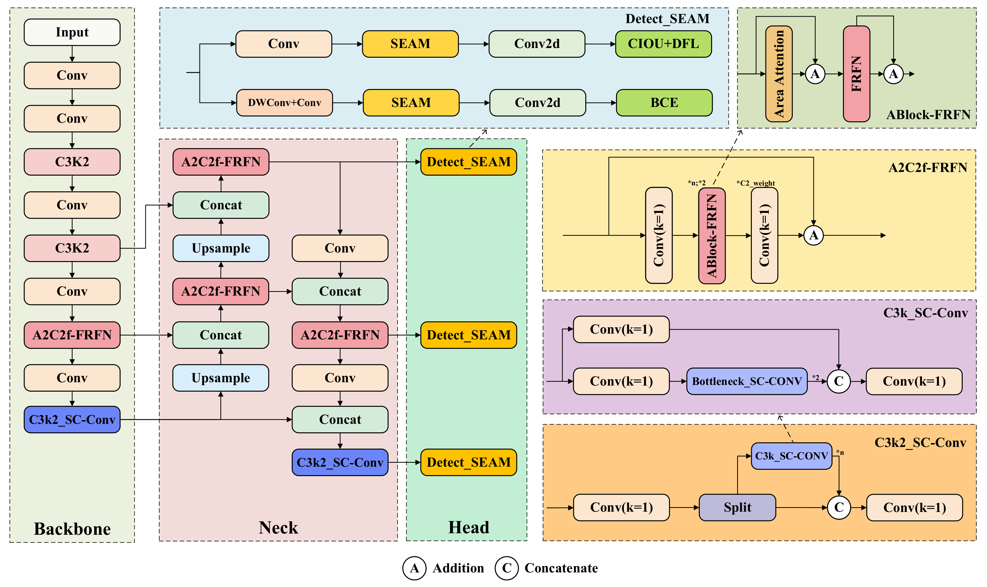
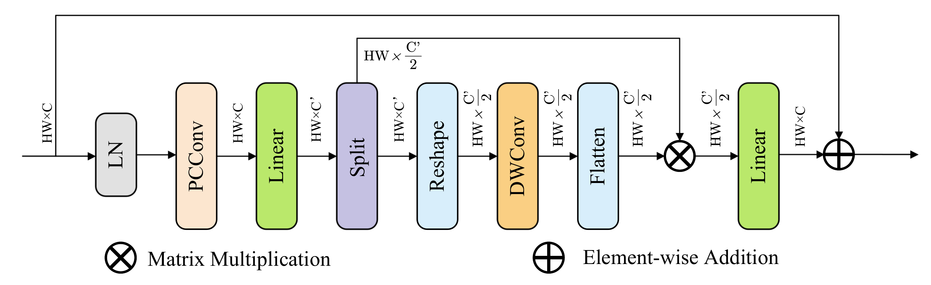
• We propose A2C2f-FRFN, an enhanced attention mechanism for the R-ELAN module in YOLOv12. This novel module integrates a Feature-Refinement Feedforward Network [19] (FRFN) to dynamically enhance spatial feature representations while suppressing redundancy, thereby improving the discriminative capacity for risky driving behaviors. This addresses the limitations of the original Area Attention by also considering channel-wise redundancy.
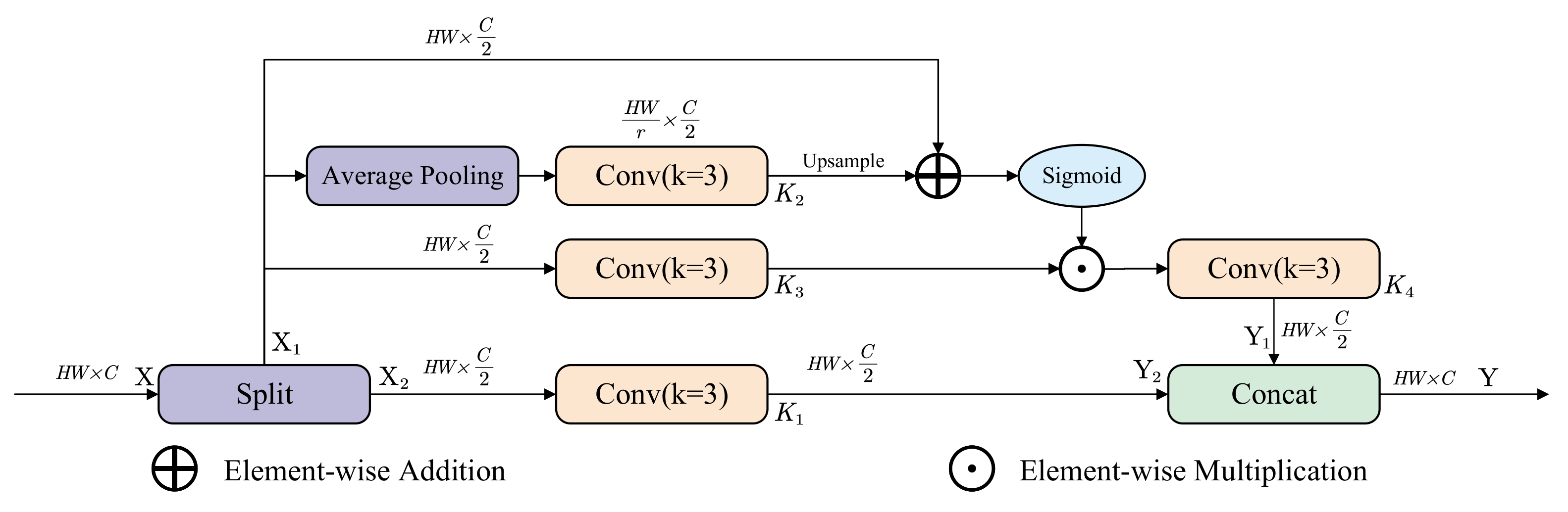
• We develop C3k2_SC-Conv structure within the backbone and neck of YOLOv12, introducing self-calibrated convolution [20] (SC-Conv). This integration broadens the receptive field and improves its ability to capture crucial contextual information for dangerous driving behavior detection without increasing computational costs. SC-Conv adaptively adjusts feature representations based on spatial and channel information, improving robustness.
• We develop Detect_SEAM by incorporating the Separated and Enhanced Attention Mechanism [21] (SEAM) into the Detect module of YOLOv12. This enhancement specifically addresses the challenges of dynamic occlusion and complex background interference common in driving scenarios. SEAM leverages depthwise separable convolution and cross-channel fusion to boost responses in unobstructed regions and compensate for occlusion-induced feature loss, improving the detection of occluded dangerous behaviors.

The rest of this paper is structured as follows: Section 2 provides an overview of dangerous driving behavior detection technologies and the YOLOv12 model. Section 3 describes the architecture and technical details of the proposed model. Section 4 presents the experimental datasets, setup, evaluation metrics, and results. Section 5 discusses the experimental results, and Section 6 concludes the study and outlines future research directions.

2. Related Works

2.1. Dangerous Driving Behavior Detection

In recent years, driven by the demand for improved road safety, the detection of dangerous driving behaviors has become a key focus of research. The goal of dangerous driving behavior detection is to assess whether a driver is in a safe driving state to prevent traffic accidents. Various methods have been proposed to address this challenge.

Vehicle behavior-based dangerous driving behavior detection methods analyze vehicle behavior characteristic parameters to extract features distinguishing normal driving from fatigued driving. These extracted parameters are used to define detection criteria to differentiate between normal and fatigued driving. Pomerleau et al. [22] proposed a Rapidly Adapting Lateral Position Handler (RALPH) system, which analyzes road images using template matching and hypothesis testing strategies to estimate lane departure information. This method is non-invasive, allows for easy data collection, and has portable detection equipment with promising market prospects. However, this detection method is susceptible to environmental factors, the driver’s skill level, and driving habits.

Physiological feature-based detection methods involve collecting physiological signals from the driver for detection. Gromer et al. [23] developed a low-cost electrocardiogram sensor that collects heart rate variability (HRV) data to detect driver fatigue. While this detection method is highly accurate and robust, it requires the use of wearable devices, which may affect the driver’s operations.

Driver feature-based detection methods assess dangerous driving by analyzing videos of the driver captured by cameras or other image sensors, usually focusing on facial features. In the absence of deep learning solutions, researchers primarily use machine vision techniques such as face recognition and facial landmark localization to extract features and detect fatigued driving. For example, Tao et al. [24] proposed a fatigue detection method based on facial alignment algorithms, utilizing six key points for each eye to locate the driver’s eyes and analyzing the eye-opening and closing states using the Adaboost algorithm to determine if the driver is fatigued.

Deep learning has been applied to driver feature detection tasks. Techniques like Deep Belief Networks (DBN), Convolutional Neural Networks (CNN), and Recurrent Neural Networks (RNN) have achieved great success in this domain [5]. With the development of R-CNN [25], SSD [26], and YOLO [27,28,29,30,31,32,33,34,35] algorithms, an increasing number of researchers have begun applying CNN-based algorithms to detect dangerous driving behaviors. Trung-Nghia Le et al. [36]. proposed the Attention R-CNN for accident identification, integrating object class and property detection with attention mechanisms. Yang et al. [37]. introduced an SSD-based method for detecting illegal driving behaviors, demonstrating superior performance over Faster R-CNN. Belmekki Ghizlene et al. [38] proposed a YOLO-Haar cascade-based method to detect driver sleepiness, incorporating an intelligent agent for real-time feedback.

Driver feature-based dangerous driving behavior detection methods offer advantages such as low cost, non-contact detection, ease of installation, compact equipment, relatively high accuracy, and the ability to detect driving dangers in real time. However, challenges arise when the driver’s head is turned too far, when wearing sunglasses, or when there is insufficient lighting, which can result in detection failures. Despite these issues, these detection methods remain dominant in the field, with a promising outlook.

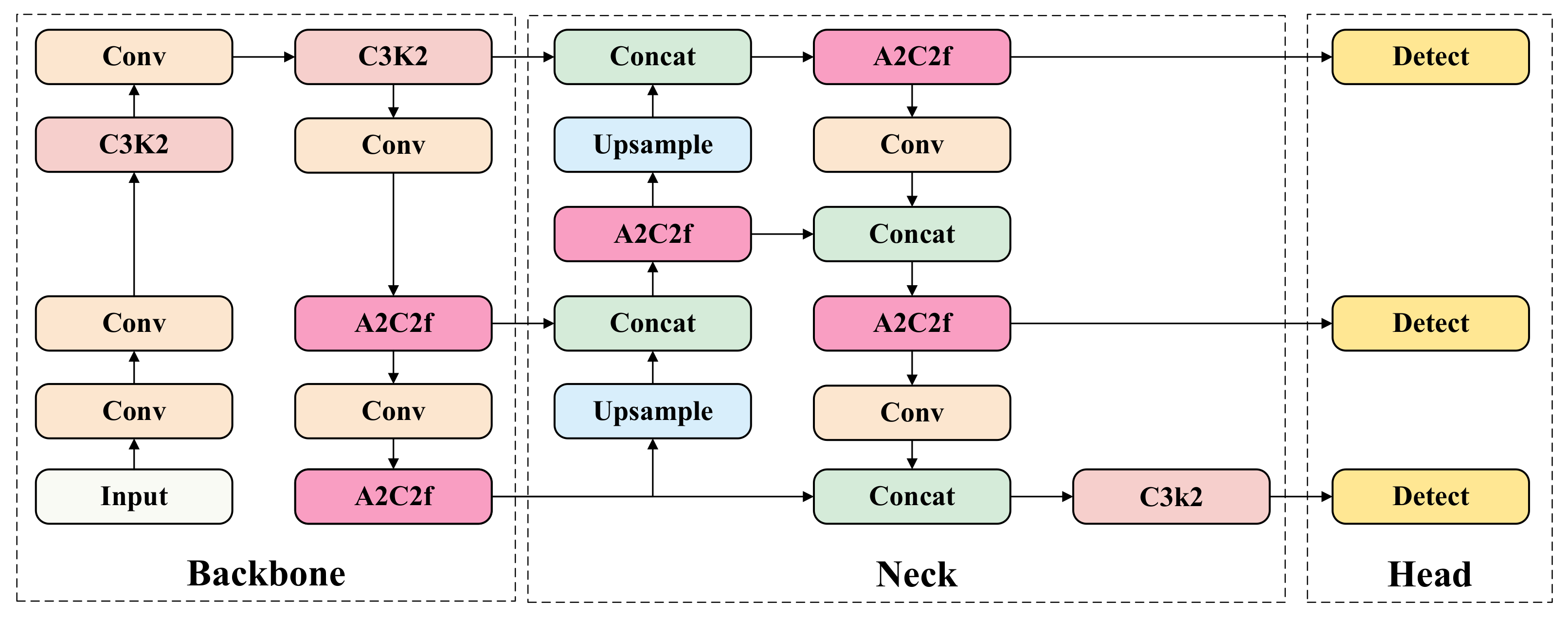
2.2. YOLOv12 Object Detection Network

YOLOv12 [35] marks the latest advancement in the YOLO series (You Only Look Once). In contrast to previous versions, YOLOv12 introduces architectural enhancements and incorporates state-of-the-art technologies, resulting in notable gains in both detection performance and computational efficiency. The model offers five different variants—n, s, m, l, and x—each with increasing network depth and detection accuracy to meet the varying needs of different applications. After a thorough assessment of factors such as detection precision, model complexity, and hardware compatibility, we chose YOLOv12-n as the base architecture for this research.

As illustrated in Figure 2, the YOLOv12 architecture includes three principal components: Backbone, Neck, and Head networks. The backbone network employs the Residual Efficient Layer Aggregation Network (R-ELAN), an enhanced variant of Efficient Layer Aggregation Network (ELAN) [30] that incorporates block-level residual connections and adaptive scaling strategies. This optimization enhances feature reuse efficiency while maintaining stable gradient propagation with minimal computational overhead. The integration of 7 × 7 large-kernel separable convolutions expands the receptive field, thus increasing the model’s ability to localize small and medium targets. Through meticulous optimization of modern GPU memory hierarchies, this architecture achieves improved computational throughput and reduced inference delay without affecting detection effectiveness.

The Neck network implements an innovative Area Attention mechanism that effectively integrates multiscale features through advanced spatial information processing. This module combines FlashAttention to address memory access challenges in attention mechanisms, enabling enhanced contextual modeling while maintaining low latency. Furthermore, the optimized multiscale feature fusion strategy improves detection accuracy across different object scales.

The detection head adopts an improved decoupled architecture from previous YOLO implementations, separating classification and localization prediction branches to mitigate inherent conflicts between these tasks. Structural innovations in the classification head replace traditional dual 3 × 3 convolutions with a two-layer depthwise separable convolution (DWConv + 1 × 1 convolution), achieving substantial reductions in model parameters while enhancing computational efficiency.

After a thorough assessment of factors such as detection precision, model complexity, and hardware compatibility, we chose YOLOv12-n as the base architecture for this research. Regarding feature fusion, YOLOv12n presents a compelling architecture. As detailed earlier in this section, its backbone employs the Residual Efficient Layer Aggregation Network (R-ELAN), and its Neck network implements an innovative Area Attention mechanism. This mechanism, which leverages FlashAttention for efficiency, effectively integrates multiscale features through advanced spatial information processing, a critical capability for our task. Dangerous driving behaviors are diverse, ranging from subtle facial cues to larger-scale actions. YOLOv12n’s optimized multiscale feature fusion strategy and attention mechanisms provide a robust foundation for capturing these varied features and their contextual information. Although newer versions such as YOLOv10 and YOLOv11 have introduced various advancements, and numerous improvement strategies exist within the field, YOLOv12-n offers a compelling balance of performance and speed, making it an ideal foundation for developing our YOLO-AFR model. Moreover, as a more recent release, YOLOv12 presents valuable opportunities for further refinement and innovation. The proposed modules—A2C2f-FRFN, C3k2_SC-Conv, and Detect_SEAM—are specifically designed to build upon this architecture, enhancing its key capabilities to enable more accurate and robust analysis of dangerous driving behaviors.

3. Methods

This section details the proposed YOLO-AFR model, which introduces three key innovations:

• The A2C2f-FRFN module incorporates the Feature-Refinement Feedback Network (FRFN) for adaptive feature refinement.
• The C3k2_SC-Conv structure utilizes self-calibrated convolution (SC-Conv) to enhance contextual modeling capability.
• The Detect_SEAM head employs the Separated and Enhanced Attention Mechanism (SEAM), designed to improve global contextual awareness.

Each of these components will be described in detail below.

3.1. A2C2f-FRFN

In the original YOLOv12 model, Area Attention was introduced to enhance the network’s ability to capture spatial information. However, when Area Attention is used as the core component for reducing spatial domain redundancy, redundancy within the channel dimension remains unaddressed. Considering the characteristics of driving scenarios—where the primary target (the driver) is clearly defined while the background is often redundant and complex, and the target scale varies significantly—we propose an improvement to the ABlock in YOLOv12’s Residual Efficient Layer Aggregation Network (R-ELAN). Specifically, we incorporate a Feature-Refinement Feedforward Network (FRFN) into the ABlock, resulting in a new module called A2C2f-FRFN, which replaces the conventional feedforward propagation structure. The proposed A2C2f-FRFN module enables dynamic enhancement of feature representations in spatial dimensions while suppressing redundancy, thereby improving the discriminative capacity of features related to risky driving behaviors.

3.1.1. Feature-Refinement Feedforward Network

The conventional Feedforward Network (FFN) processes information at each pixel location individually, playing a crucial role in improving feature representation through self-attention mechanisms. Therefore, designing an effective feedforward network to enhance features and drive potential high-quality image recovery is critical.

To overcome this issue, we introduce a Feature-Refinement Feedforward Network (FRFN), which performs feature transformation through an enhancement-relief paradigm. Specifically, we strengthen the information elements within the features by incorporating a partial convolution (PConv) operation and use an adaptive gating subsystem to automatically suppress feature channels with high redundancy coefficients, thereby achieving dynamic computation allocation during information processing. The FRFN can be represented as:

$${\widehat{X}}^{\prime }=\mathrm{GELU}\left(W_1\mathrm{PConv}\left(\widehat{X}\right)\right),[{\widehat{X}}_1^{\prime },{\widehat{X}}_2^{\prime }]={\widehat{X}}^{\prime },$$

(1)

$${\widehat{X}}_r^{\prime }={\widehat{X}}_1^{\prime }\otimes \mathrm{F}\left(\mathrm{DWConv}\left(\mathrm{R}\left({\widehat{X}}_2^{\prime }\right)\right)\right),$$

(2)

$${\widehat{X}}_{\mathrm{out}}^{\prime }=\mathrm{GELU}\left(W_2{\widehat{X}}_r^{\prime }\right),$$

(3)

where $W_1$ and $W_2$ represent linear projection matrices; the operator $[,]$ denotes channel-wise slicing; $\mathrm{R}(·)$ and $\mathrm{F}(·)$ correspond to the Reshape and Flatten operations, respectively, transforming sequential inputs into 2D feature maps (and vice versa), a key mechanism for introducing locality into the architecture; $\mathrm{PConv}(·)$ and $\mathrm{DWConv}(·)$ indicate partial convolution and depthwise convolution operations; and the symbol ⊗ denotes matrix multiplication. The input features (HW × C) are first normalized through Layer Normalization (LN), then processed by partial convolution (PConv) and linear transformation for dimension adjustment. Subsequently, the features are split into two parallel branches: one branch extracts local patterns through depthwise separable convolution (DWConv), while the other preserves the original information flow. These two branches are fused via element-wise multiplication, followed by another linear transformation to restore the original dimensionality. Finally, the processed features are combined with the initial input through residual connection, yielding refined output features. The architecture is illustrated in Figure 3.

The Feature-Refinement Fusion Network (FRFN) enhances representation capability by distilling discriminative features from information flow while suppressing redundant components, effectively implementing feature selection at the channel level. This architecture further provides an explicit pathway for the model to eliminate uninformative features along channel dimensions through its dual-branch design.

3.1.2. Structure of A2C2f-FRFN

Among the architectural enhancements in YOLOv12, the Residual Efficient Layer Aggregation Network (R-ELAN) represents a significant innovation. Departing from conventional designs, this module introduces a residual shortcut connection spanning from input to output with an additional scaling factor (default value 0.01). The architecture first employs transition layers to adjust channel dimensions, generating unified feature maps. These processed features subsequently undergo multi-submodule transformations before concatenation with original features, forming an optimized bottleneck structure that substantially enhances feature representation effectiveness. This architecture is integrated with the Area Attention mechanism to create a novel composite module (denoted as A2C2f in YOLOv12’s official implementation), replacing the legacy C3k2 modules from previous YOLO iterations.

Notably, the ABlock module housing Area Attention employs a Multi-Layer Perceptron (MLP) for feature transformation. In YOLOv12’s implementation, the channel expansion ratio was strategically reduced from 4 to 1.2 (2 for N-/S-/M-scale models) to optimize computational resource allocation. While this modification improves operational efficiency, it risks compromising attention effectiveness through excessive parameter simplification. To address this limitation, we propose replacing the original MLP structure with a Feature-Refinement Feedback Network (FRFN). This substitution enhances both feature extraction capability and redundant information elimination, thereby fully realizing the potential of Area Attention. The enhanced architecture (ABlock-FRFN) subsequently forms the basis for our proposed A2C2f-FRFN module as a superior alternative to the original A2C2f configuration.

The A2C2f-FRFN module adeptly synergizes the spatial feature representation enhancement capabilities inherent in the original A2C2f structure with the distinct advantages of FRFN in refining features and suppressing redundancy. This synergy enables the module to dynamically enhance spatial feature representations while effectively curtailing information redundancy. The architecture of A2C2f-FRFN is illustrated in Figure 1.

3.2. C3k2_SC-Conv

Traditional convolution operations have inherent limitations. One issue is the similarity in convolution kernel learning modes, which limits the diversity of feature extraction. Another limitation is that the receptive field at each spatial location is primarily governed by the fixed size of the convolution kernel, which restricts the network’s capacity to capture broader contextual information. This restriction results in a smaller receptive field, hampering the network’s ability to capture high-level semantic features. As a consequence, the performance of feature recognition is diminished, impacting the overall accuracy of the model.

To overcome these challenges, we introduce self-calibrated convolution (SC-Conv) into both the backbone and neck of the original YOLOv12 architecture. This enhancement significantly improves the receptive field for target features, which in turn boosts the model’s detection accuracy. The structure of SC-Conv is depicted in Figure 4.

3.2.1. Self-Calibrated Convolutions

The self-calibration mechanism within SC-Conv allows the model to dynamically adjust feature representations based on spatial and channel-specific information. This adaptability improves the robustness of object detection. Moreover, SC-Conv enhances the performance of conventional convolutional layers without adding extra parameters or increasing computational complexity. Its straightforward, plug-and-play design makes it easy to integrate into existing neural network frameworks.

To efficiently and effectively gather valuable contextual information for each spatial location, self-calibrated convolution uses convolutional feature transformations in two different spatial scales: one is the original scale space where the feature map retains the same resolution as the input, and the other is a downsampled latent space.

As illustrated in Figure 4, SC-Conv begins by partitioning the input X into two parts, denoted as $X_1$ and $X_2$. These two parts are then fed into specialized paths to extract different types of contextual information. Among them, $X_1$ undergoes a self-calibration operation to obtain $Y_1$. In this process, the parameter r dynamically adjusts the receptive field for each spatial position, enabling the model to capture deep semantic knowledge from distant spatial locations and channels, thus enhancing the diversity of the output features. Meanwhile, $X_2$ undergoes a simple convolution operation to obtain $Y_2$, preserving the original spatial contextual relationships. Finally, the intermediate outputs $Y_1$ and $Y_2$ are concatenated to produce the final output Y. Specifically, self-calibration, as described in the upper part of the figure, begins with the output $X_1$. We perform average pooling with a filter size of $s\times s$ and a stride of s, as follows:

$$M_1={\mathrm{AvgPool}}_r\left(X_1\right).$$

(4)

The feature transformation in $M_1$ is based on $K_2$:

$$X_1^{\prime }=\mathrm{Upsample}(T_1\ast K_2),$$

(5)

where $\mathrm{Upsample}(·)$ is an operator that uses bilinear interpolation to map the intermediate reference from the reduced-scale space back to the original feature space. This operation can then be written as:

$$Y_1^{\prime }=X_1\ast K_3·\sigma (X_1+X_1^{\prime }),$$

(6)

where $\sigma$ represents the sigmoid function, and the “·” denotes element-wise multiplication. As shown in Equation (6), $X_1^{\prime }$ is used as a residual to form the calibration weight. The final calibrated output can be written as:

$$Y_1=Y_1^{\prime }\ast K_4.$$

(7)

The self-calibration mechanism within SC-Conv is pivotal, allowing the model to dynamically adjust feature representations based on both spatial positions and channel-specific information. This adaptability significantly improves the robustness of object detection tasks. Specifically for dangerous driving behavior detection, the self-calibration operation effectively expands the receptive field by considering local context and modeling channel dependencies. This enhanced contextual awareness is crucial, enabling the model to capture a broader scene that includes driver actions, facial expressions, and changes in the vehicle’s environment, thereby overcoming the limited receptive field of conventional convolution and leading to more effective identification of diverse dangerous driving cues, from subtle micro-expressions to larger actions. Crucially, SC-Conv achieves these enhancements in feature representation and receptive field without introducing additional parameters or increasing computational complexity when compared to standard convolutions. This is a significant advantage over many alternative approaches that attempt to achieve similar benefits—such as an expanded receptive field or sophisticated feature dependency modeling—by incorporating separate, learnable modules (e.g., attention mechanisms) or a greater number of filters, which inevitably escalate the computational cost. SC-Conv, instead, leverages its intrinsic self-calibration process to efficiently re-weight and refine features, primarily by reconfiguring the use of existing filter information rather than adding new parameterized layers. Furthermore, its straightforward, plug-and-play nature facilitates easy integration into existing neural network architectures, making it a practical solution for improving model performance without a heavy computational overhead.

3.2.2. Architecture Development of C3k2_SC-Conv

We replace the second convolution in the CBS block with SC-Conv to enhance the BottleNeck structure, which we refer to as BottleNeck_SC. Subsequently, stacking N sets of BottleNeck_SC forms the C3k_SC-Conv structure. Then, C3k_SC-Conv is used to replace C3k in the original C3k2 module, resulting in C3k2_SC-Conv. Due to the larger receptive field of SC-Conv, C3k2_SC-Conv can more accurately locate dangerous driving behaviors within the in-vehicle environment. The structure of C3k2_SC-Conv is shown in Figure 1. Specifically, we adopt the C3k2_SC-Conv structure in the P5 layer of the original network. This involves replacing part of the standard convolution in the C3k2 structure with SC-Conv to enhance the feature extraction capability of the network.

3.3. Detect_SEAM

Focusing on the critical issues of real-time partial occlusions and multi-source interference in driver monitoring systems, we propose a vision enhancement framework by embedding the Separated and Enhanced Attention Mechanism (SEAM) into the YOLOv12 architecture. This adaptation draws from SEAM’s proven effectiveness in occlusion management through its successful implementation in facial recognition systems (YOLO-FaceV2), making it particularly suitable for detecting facial-related dangerous behaviors (e.g., yawning and eye-closing) and frequently occluded objects (e.g., mobile phones and water bottles obscured by steering wheels) in driving scenarios.

3.3.1. Separated and Enhancement Attention Module

The Separated and Enhancement Attention Module (SEAM) is designed to enhance feature representation, particularly for accurately detecting driver behavior by compensating for occlusion-induced feature loss. At the core of SEAM is the Channel and Spatial Mixing Module (CSMM). The CSMM utilizes different patch configurations to capture multiscale contextual features. Within each CSMM, depthwise separable convolution (DWconv) is employed to efficiently learn the correlation of spatial dimensions and channels. If $X_{in}$ represents the input to a feature extraction block, a residual depthwise convolution operation can be formulated as:

$$X_{res}^{\prime }=X_{in}+\mathcal{B}\left(\mathrm{GELU}\left({\mathrm{Conv}}_{dw}(X_{in};W_{dw})\right)\right)$$

(8)

Depthwise separable convolution operates on individual input channels to learn channel-specific spatial importance, which significantly reduces the parameter count compared to standard convolutions. However, a characteristic of processing channels independently in this manner is that it initially neglects inter-channel relationships. To address this limitation and strengthen inter-channel dependencies, SEAM integrates a cross-channel fusion mechanism. Specifically, the outputs of channel-wise spatial convolutions (from the depthwise component) are effectively combined using $1\times 1$ pointwise convolutions. Subsequently, a two-layer fully connected network is employed to aggregate global cross-channel information. This layered approach strengthens inter-channel dependencies, enabling effective compensation for feature loss caused by occlusion through learned correlations between occluded and non-occluded regions.

As illustrated in Figure 5, the overall SEAM architecture processes an initial feature tensor through three distinct CSMMs, each configured with divergent patch parameters. These processed signals are subsequently aggregated with the original features through element-wise summation. This aggregated representation then undergoes spatial averaging via global pooling. The condensed feature representation traverses a dual-layer neural network comprising two cascaded fully connected architectures, which collaboratively generate a channel-wise attention-weighting matrix. Finally, the module’s output is obtained by performing element-wise multiplication between this attention-weighting matrix (appropriately broadcast) and the original input feature map.

This architectural design, particularly the use of depthwise separable convolutions within the CSMMs, leads to substantial model compression. For instance, a conventional convolutional layer with identical input/output dimensions (c channels) and kernel width k requires a significant number of trainable parameters (on the order of $c^2·k^2$). Through the decomposed implementation inherent in depthwise separable convolution, this complexity is strategically distributed into two main components: spatial feature extraction (the depthwise part, requiring parameters on the order of $c·k^2$) and cross-channel information fusion via pointwise convolutions (requiring parameters on the order of $c^2$, assuming consistent channel dimensions). This cumulative reduction yields significantly lower parametric demands, proving particularly advantageous for embedded deployment scenarios requiring instantaneous response in driver behavior detection.

As illustrated in Figure 5, the initial feature tensor undergoes parallel processing through three distinct CSMM configured with divergent patch configurations (where patch parameters govern the padding strategies applied to the feature map) [39]. These processed signals are subsequently aggregated with the original features through element-wise summation before proceeding to spatial averaging via global pooling. The condensed feature representation then traverses a dual-layer neural network comprising two cascaded fully connected architectures, which collaboratively generate a channel-wise attention-weighting matrix. Finally, the output is obtained by performing element-wise multiplication between the adjusted feature map and the original input feature map.

3.3.2. Construction of Detect_SEAM

In the YOLOv12 model, the Detect module handles the last detection stage. By incorporating SEAM into the second Convolution-BatchNorm-Silu block of the original Detect module, we improve the model’s focus on crucial features before proceeding to the last classification and regression stages. This adjustment improves the ability to identify and accurately pinpoint facial behaviors that are partially obscured during driving. The original detection head, Detect, is substituted with an enhanced version, Detect_SEAM. The structure of Detect_SEAM is illustrated in Figure 1.

4. Experiments and Analysis

4.1. Experimental Dataset

To comprehensively assess the detection performance of the YOLO-AFR model across various scenarios and behavior scales, this study adopts the same two publicly available datasets, encompassing six categories of dangerous driving behaviors of different scales. These datasets are the YawDD-E and SfdDD datasets. The YawDD-E dataset is composed of three sub-datasets: YawDD [40], VOC-COCO [41], and DrivFace [42], containing a total of 2951 images captured from a frontal view within the vehicle. To ensure a fair evaluation and enhance the model’s generalization ability across different individuals, we adopted a cross-driver split strategy, whereby images of the same driver do not appear in both the training and test sets. The SfdDD [43] dataset consists of 3900 images taken from a side-view perspective and a similar cross-driver partitioning was applied. This approach allows for a more robust evaluation of the model’s capacity to detect dangerous driving behaviors performed by different drivers. The distribution of labeled categories in each dataset is presented in

Table 1. The distribution of labeled categories in the study. “~” means this category is not present in the dataset.

Dataset	Closed Eyes	Yawn	Playing Phone	Drinking	Single Hand
YawDD-E	1177	1385	1269	~	~
SfdDD	~	~	1597	1700	3053

. Representative samples from the dataset are shown in Figure 6.

4.2. Experimental Environment

All computational tasks in this research were executed on a dedicated server utilizing an AMD EPYC 7502 processing unit paired with an NVIDIA GeForce RTX 3090 graphics card (24 GB VRAM), supported by 16 GB RAM to manage computational workloads. The system operated on a Linux-based platform. For accelerated neural network operations, the implementation leveraged the PyTorch 2.2.2 framework integrated with CUDA 12.1 acceleration and Python 3.10 runtime environment.

The optimization protocol employed the AdamW algorithm initialized with a learning rate of 0.001429, accompanied by momentum stabilization at 0.9 and a weight decay coefficient of 0.0005. Training procedures spanned 300 complete iterations of the dataset with mini-batch processing configured to 16 samples per batch.

4.3. Evaluation Metrics

To evaluate the performance of the proposed models, we adopt several key metrics: Precision, Recall, F1 Score, and mean Average Precision (mAP). Additionally, model complexity is assessed based on GFLOPs (Giga Floating Point Operations), Frames Per Second (FPS), the number of parameters (M) and the weight size.

Precision is defined as the proportion of correctly predicted positive samples among all samples predicted as positive. It reflects the accuracy of the model’s positive predictions and is calculated as:

$$\mathrm{Precision}={\displaystyle \frac{TP}{TP+FP}}$$

(9)

where $TP$ (True Positives) denotes the number of correctly predicted positive samples and $FP$ (False Positives) refers to the number of negative samples incorrectly predicted as positive.

Recall measures the proportion of actual positive samples that are correctly identified by the model, indicating its ability to capture positive instances. It is defined as:

$$\mathrm{Recall}={\displaystyle \frac{TP}{TP+FN}}$$

(10)

where $FN$ (False Negatives) denotes the number of positive samples incorrectly predicted as negative.

The F1 Score is the harmonic mean of precision and recall, providing a balanced evaluation metric, especially valuable in imbalanced datasets. It is calculated as:

$$F1={\displaystyle \frac{2\times P\times R}{P+R}}$$

(11)

Average Precision (AP) is computed as the area under the precision-recall curve, derived from the IoU (Intersection over Union) score between the predicted and actual bounding boxes. It is defined as:

$$\mathrm{AP}=\sum _{i=1}^{n}P\left(i\right)·\Delta R\left(i\right)$$

(12)

where $P\left(i\right)$ is the precision at the i-th threshold, and $\Delta R\left(i\right)$ is the change in recall at that threshold.

Mean Average Precision (mAP) is the average of APs across all classes. Specifically, mAP@0.5 refers to AP computed at an IoU threshold of 0.50, while mAP@0.5:0.95 averages AP over multiple IoU thresholds from 0.50 to 0.95 with a step size of 0.05. The overall mAP is given by:

$$\mathrm{mAP}={\displaystyle \frac{1}{n}}\sum _{c=1}^{n}A{P}_c$$

(13)

where n is the total number of classes, and $A{P}_c$ is the average precision for class c.

4.4. Model Comparison Experiment

4.4.1. Comparison of Detection Accuracy Across Models

To evaluate the performance of different detection models on the SfdDD and YawDD-E datasets, we compared a variety of models, including Faster R-CNN [44], SSD [26], YOLOv3-tiny [27], YOLOv5n [28], YOLOv6n [29], YOLOv7-tiny [30], YOLOv8n [31], YOLOv9-C [32], YOLO-SGC [15], YOLOv10n [33], YOLOv11n [34], and YOLOv12n [35]. We also compare other computer vision-based dangerous driving behavior detection models proposed by researchers.

The results of the experiments are displayed in

Table 2. Performance comparison on the YawDD-E dataset. The top results for each metric are shown in bold, with the next best results underlined.

Methods	mAP@0.5	mAP@0.5:0.95	Precision	Recall	F1-Score
Faster R-CNN	0.557	0.352	0.541	0.601	0.569
SSD	0.879	0.507	0.865	0.842	0.853
YOLOv3-tiny	0.935	0.698	0.884	0.864	0.874
YOLOv5n	0.934	0.706	0.892	0.869	0.880
YOLOv6n	0.950	0.734	0.895	0.891	0.893
YOLOv7-tiny	0.934	0.728	0.923	0.863	0.892
YOLOv8n	0.952	0.764	0.933	0.879	0.905
YOLOv9-C	0.962	0.772	0.945	0.890	0.917
YOLO-SGC	0.972	0.793	0.949	0.908	0.928
YOLOv10n	0.960	0.738	0.900	0.943	0.920
YOLOv11n	0.963	0.742	0.922	0.922	0.920
YOLOv12n	0.963	0.737	0.928	0.920	0.922
YOLO-AFR	0.976	0.763	0.936	0.947	0.940

and

Table 3. Performance comparison on the SfdDD dataset. The top results for each metric are shown in bold, with the next best results underlined.

Methods	mAP@0.5	mAP@0.5:0.95	Precision	Recall	F1-Score
Faster R-CNN	0.663	0.512	0.661	0.666	0.663
SSD	0.933	0.551	0.937	0.942	0.939
YOLOv3-tiny	0.958	0.560	0.955	0.957	0.956
YOLOv5n	0.954	0.543	0.943	0.940	0.941
YOLOv6n	0.964	0.563	0.964	0.944	0.951
YOLOv7-tiny	0.968	0.548	0.967	0.968	0.967
YOLOv8n	0.970	0.586	0.958	0.962	0.960
YOLOv9-C	0.983	0.590	0.978	0.988	0.983
YOLO-SGC	0.980	0.596	0.976	0.982	0.979
YOLOv10n	0.966	0.586	0.947	0.953	0.950
YOLOv11n	0.972	0.590	0.961	0.961	0.961
YOLOv12n	0.971	0.575	0.950	0.960	0.954
YOLO-AFR	0.989	0.698	0.978	0.982	0.980

. Our model outperforms the other 12 detection models on both the YawDD-E public dataset (for frontal-view detection) and the SfdDD public dataset (for side-view detection). Specifically, our model achieves the highest mAP@0.5 across all models, with a 0.4–75.9% improvement in mAP@0.5 on YawDD-E and a 0.6–49.2% improvement on SfdDD. In addition, YOLO-AFR excels in other metrics as well. On the SfdDD dataset, YOLO-AFR improves the mAP@0.5:0.95 by 0.1 over the previous SOTA model, YOLO-SGC, and achieves the highest precision among all models, significantly outperforming the others. On the YawDD-E dataset, YOLO-AFR achieves the highest recall and F1 score, demonstrating its robust capability in dangerous driving behavior detection tasks.

From

Table 4. mAP@0.5 Comparison of Different Detection Methods on the YawDD Dataset. The top results for each metric are shown in bold, with the next best results underlined.

Model	Narayanan et al. [45]	Yang et al. [46]	Kir et al. [47]	Dong et al. [48]	Bai et al. [49]	Alameen et al. [50]	Li et al. [51]	YOLO-SGC [17]	YOLO-AFR
mAP@0.5	0.818	0.834	0.880	0.910	0.934	0.960	0.944	0.972	0.976

and

Table 5. mAP@0.5 Comparison of Different Detection Methods on the SfdDD Dataset. The top results for each metric are shown in bold, with the next best results underlined.

Model	Abouelnaga et al. [52]	Baheti et al. [53]	Qin et al. [54]	Li et al. [55]	Shang et al. [56]	Gao et al. [57]	Chillakuru et al. [58]	YOLO-SGC [17]	YOLO-AFR
mAP@0.5	0.937	0.952	0.956	0.949	0.946	0.935	0.976	0.980	0.989

, it is evident that our model outperforms 14 other recently proposed dangerous driving behavior detection models on both the YawDD-E front-view dataset and the SfdDD side-view dataset. Specifically, our model achieves an improvement in the mAP@0.5 metric by 0.41% to 19.3% on YawDD-E and by 0.92% to 5.77% on SfdDD, surpassing other models and highlighting its exceptional accuracy in detecting dangerous driving behaviors. Furthermore, while the models discussed in the related literature are unable to simultaneously detect dangerous driving behaviors from both frontal and side views, our model excels in handling both perspectives, demonstrating remarkable adaptability and versatility.

To rigorously assess whether the accuracy enhancements of YOLO-AFR are statistically significant compared to other relevant models discussed in this paper, we performed an independent samples t-test. This analysis specifically compared the mAP@0.5 scores of YOLO-AFR against those of YOLO-SGC, the second-best performing model, utilizing data from the final 20 training epochs on both the SfdDD and YawDD-E datasets. The detailed results of these statistical tests are presented in

Table 6. Statistical Comparison of mAP@0.5 for YOLO-SGC and YOLO-AFR on YawDD-E Dataset.

Metric	Group	N	Mean	SD	t-Test	Welch’s t-Test	Mean Diff.	Cohen’s d
mAP@0.5	YOLO-SGC	20	0.969	0.003	T = −6.953	T = −6.953	0.004	2.199
	YOLO-AFR	20	0.973	0.001	p < 0.001	p < 0.001
	Total	40	0.971	0.003

(for the YawDD-E dataset) and

Table 7. Statistical Comparison of mAP@0.5 for YOLO-SGC and YOLO-AFR on SfdDD Dataset.

Metric	Group	N	Mean	SD	t-Test	Welch’s t-Test	Mean Diff.	Cohen’s d
mAP@0.5	YOLO-SGC	20	0.977	0.003	T = 11.815	T = 11.815	0.008	3.736
	YOLO-AFR	20	0.985	0.002	p < 0.001	p < 0.001
	Total	40	0.981	0.005

(for the SfdDD dataset). In both instances, the p-values were found to be less than 0.001 (p < 0.001), providing strong statistical evidence that the precision achieved by YOLO-AFR is significantly superior to that of YOLO-SGC.

4.4.2. Comparison of Model Efficiency and Complexity

To comprehensively evaluate the practical performance of our model in dangerous driving behavior detection, we conducted experiments on the SfdDD dataset, comparing YOLO-AFR with several representative models, including YOLO-SGC, YOLOv10n, YOLOv11n, and YOLOv12n. The comparison covers key performance metrics such as computational complexity (GFLOPs), number of parameters, inference speed, frames per second (FPS), and model weight size. The results are shown in

Table 8. Comparison of model complexity, speed, and file size.

Model	GFLOPs	Parameters (M)	Speed (ms)	FPS	Weight Size (MB)
YOLO-SGC	23.4	8.832	13.61	73.50	5.2
YOLOv10n	6.5	2.266	9.54	104.82	5.5
YOLOv11n	6.3	2.583	8.12	123.21	5.2
YOLOv12n	6.3	2.557	10.40	96.17	5.3
YOLO-AFR	5.7	2.421	9.56	104.59	5.0

.

As illustrated in the table, YOLO-AFR demonstrates significant advantages across multiple dimensions. It has the lowest computational complexity (only 5.7 GFLOPs), a compact parameter size of 2.421 M, and achieves an inference speed of 104.59 FPS, with a weight size of just 5.0 MB. This allows YOLO-AFR to maintain high accuracy while delivering exceptional efficiency and deployment flexibility.

These performance metrics are especially critical in the domain of dangerous driving behavior detection. Traffic scenarios are often highly dynamic, requiring models with high frame rates and low latency to ensure timely alerts. Additionally, lightweight models are essential for deployment on in-vehicle or edge devices. By striking a balance between accuracy, speed, and resource efficiency, YOLO-AFR proves to be highly suitable and powerful for real-world driving safety applications.

To comprehensively evaluate the performance of our proposed YOLO-AFR model, Figure 7 presents a comparative analysis against several other contemporary real-time object detectors—YOLO-SGC, YOLOv12n, YOLOv11n, and YOLOv10n—on the SfdDD dataset. As depicted in the figure, our YOLO-AFR model demonstrates a compelling advantage, achieving the highest detection accuracy while maintaining a high inference speed and, notably, the lowest GFLOPs, thereby underscoring its superior overall performance and efficiency.

4.5. Ablation Experiment

To evaluate the performance of our modules—SEAM (A), FRFN (B), and SC-Conv (C)—we conducted extensive ablation experiments on two datasets with different perspectives: the side-view driving behavior dataset SfdDD and the front-view dataset YawDD-E. The results are summarized in

Table 9. Quantitative comparison of ablation experimental results on the SfdDD dataset. The top results for each metric are shown in bold, with the next best results underlined.

Method	SEAM	FRFN	SC-Conv	Category	Precision	Recall	F1-Score	AP@0.5	AP@0.5:0.95	mAP@0.5
None				Playing phone	0.933	0.936	0.934	0.963	0.464	0.971
				Drinking	0.930	0.969	0.949	0.958	0.543
				Single hand	0.986	0.973	0.980	0.991	0.719
A	🗸			Playing phone	0.916	0.936	0.926	0.940	0.574	0.972
				Drinking	0.979	0.980	0.979	0.984	0.684
				Single hand	0.990	0.967	0.978	0.992	0.800
B		🗸		Playing phone	0.926	0.927	0.927	0.949	0.596	0.973
				Drinking	0.962	0.973	0.968	0.979	0.691
				Single hand	0.993	0.978	0.986	0.991	0.802
C			🗸	Playing phone	0.956	0.959	0.957	0.965	0.571	0.979
				Drinking	0.970	0.973	0.972	0.982	0.689
				Single hand	0.987	0.968	0.977	0.992	0.805
A + B	🗸	🗸		Playing phone	0.947	0.960	0.954	0.968	0.595	0.977
				Drinking	0.957	0.973	0.965	0.971	0.677
				Single hand	0.994	0.967	0.980	0.992	0.797
A + C	🗸		🗸	Playing phone	0.937	0.955	0.946	0.958	0.600	0.974
				Drinking	0.947	0.969	0.958	0.972	0.661
				Single hand	0.981	0.990	0.986	0.993	0.800
B + C		🗸	🗸	Playing phone	0.953	0.951	0.952	0.965	0.575	0.980
				Drinking	0.967	0.966	0.966	0.980	0.683
				Single hand	0.984	0.971	0.977	0.991	0.811
A + B + C	🗸	🗸	🗸	Playing phone	0.969	0.988	0.978	0.987	0.600	0.989
				Drinking	0.979	0.984	0.982	0.988	0.695
				Single hand	0.985	0.972	0.978	0.990	0.799

and

Table 10. Quantitative comparison of ablation experimental results on the YawDD-E dataset. The top results for each metric are shown in bold, with the next best results underlined.

Method	SEAM	FRFN	SC-Conv	Category	Precision	Recall	F1-Score	AP@0.5	AP@0.5:0.95	mAP@0.5
None				Yawn	0.877	0.977	0.924	0.975	0.809	0.963
				Closed eyes	0.926	0.867	0.896	0.954	0.770
				Playing phone	0.982	0.916	0.948	0.961	0.632
A	🗸			Yawn	0.868	0.971	0.917	0.975	0.819	0.973
				Closed eyes	0.927	0.913	0.920	0.962	0.775
				Playing phone	0.955	0.951	0.953	0.981	0.667
B		🗸		Yawn	0.836	0.994	0.908	0.977	0.809	0.969
				Closed eyes	0.930	0.927	0.929	0.957	0.784
				Playing phone	0.956	0.944	0.950	0.973	0.657
C			🗸	Yawn	0.904	0.966	0.934	0.977	0.826	0.970
				Closed eyes	0.944	0.874	0.908	0.965	0.769
				Playing phone	0.977	0.895	0.934	0.969	0.636
A + B	🗸	🗸		Yawn	0.882	0.986	0.931	0.977	0.823	0.971
				Closed eyes	0.917	0.911	0.914	0.962	0.775
				Playing phone	0.964	0.935	0.949	0.974	0.667
A + C	🗸		🗸	Yawn	0.853	0.989	0.916	0.972	0.815	0.972
				Closed eyes	0.907	0.937	0.922	0.965	0.788
				Playing phone	0.939	0.967	0.953	0.977	0.678
B + C		🗸	🗸	Yawn	0.865	0.989	0.923	0.978	0.820	0.973
				Closed eyes	0.926	0.909	0.917	0.962	0.780
				Playing phone	0.955	0.965	0.960	0.978	0.665
A + B + C	🗸	🗸	🗸	Yawn	0.874	0.989	0.928	0.980	0.828	0.976
				Closed eyes	0.953	0.887	0.919	0.961	0.797
				Playing phone	0.981	0.965	0.973	0.986	0.663

.

From the results on the SfdDD dataset, it is evident that incorporating any of the three modules individually leads to noticeable performance improvements across different behavior categories. Specifically, the SEAM module significantly boosts performance for the “Drinking” category, increasing Precision from 0.930 to 0.979 and improving AP@0.5 to 0.984. This demonstrates SEAM’s effectiveness in capturing temporal contextual information. The FRFN module shows improvements in overall AP@0.5:0.95 scores, particularly for the “Drinking” category as well, where AP@0.5:0.95 reaches 0.691, validating its strength in multiscale feature fusion. The SC-Conv module enhances the model’s focus on spatially relevant regions, with overall mAP@0.5 achieving 0.979, indicating its contribution to spatial localization accuracy.

When any two modules are combined (A + B, A + C, or B + C), further performance gains are observed due to their complementary effects. For example, the combinations A+B and B+C reach mAP@0.5 scores of 0.977 and 0.980, respectively, outperforming the single-module configurations. The complete integration of all three modules is our proposed YOLO-AFR model (A + B + C), which achieves the best results on the SfdDD dataset, with mAP@0.5 increasing to 0.989, a 1.8% improvement over the baseline YOLOv12. Notably, in the challenging ’Playing phone’ and ’Drinking’ categories, AP@0.5:0.95 reaches 0.600 and 0.695, demonstrating robust detection capability for fine-grained behaviors and small targets.

A similar trend is observed in the YawDD-E dataset. Each individual module contributes positively, with SC-Conv particularly effective in the “Yawn” category, raising the F1-Score to 0.934 and AP@0.5:0.95 to 0.826. The FRFN module enhances recall and overall mAP@0.5 in “Closed eyes”, while SEAM consistently improves AP@0.5 and AP@0.5:95 across all categories, confirming its strength in modeling temporal consistency. When all three modules are combined, the YOLO-AFR model achieves a mAP@0.5 of 0.976, surpassing the baseline by 1.3%, respectively, while maintaining balanced performance across categories. These results highlight the model’s strong generalization ability and robustness under various viewpoints. Figure 8 illustrates the enhancement of mAP@0.5 gains on both the SfdDD and YawDD-E datasets as key components are integrated.

Figure 9 illustrates the synergistic interaction of the FRFN, SC-Conv, and SEAM modules, pivotal to YOLO-AFR’s enhanced performance.

In the backbone and neck, SC-Conv first calibrates features—expanding receptive fields and bolstering context—then passes them to FRFN for refinement. FRFN’s output is subsequently recalibrated by SC-Conv, forming an iterative “Calibration-Refinement Loop”. This loop executes multiple times, progressively reducing redundancy and enhancing discriminative features layer by layer.

This iterative process yields multiscale features (P3, P4, P5) with varying receptive fields and semantic strengths: P3 (smallest field, shallowest semantics) offers high localization precision; P4 balances semantics and localization; and P5 (largest field, richest semantics) is ideal for global context and large-scale targets.

Subsequently, in the head, the SEAM module unifies these optimized P3, P4, and P5 features into a common contextual space. This ensures consistent prediction logic across all target sizes, significantly mitigating cross-scale conflicts and occlusion-based misdetections.

Together, FRFN, SC-Conv, and SEAM create a hierarchically complementary, information-enhancing framework, which is fundamental to achieving YOLO-AFR’s characteristic high precision and robustness.

In conclusion, each of the proposed modules contributes significantly to the overall performance, and their joint integration yields a synergistic effect. The final YOLO-AFR model (A + B + C) consistently outperforms the baseline YOLOv12 on both datasets, validating the effectiveness and generalizability of the proposed architecture.

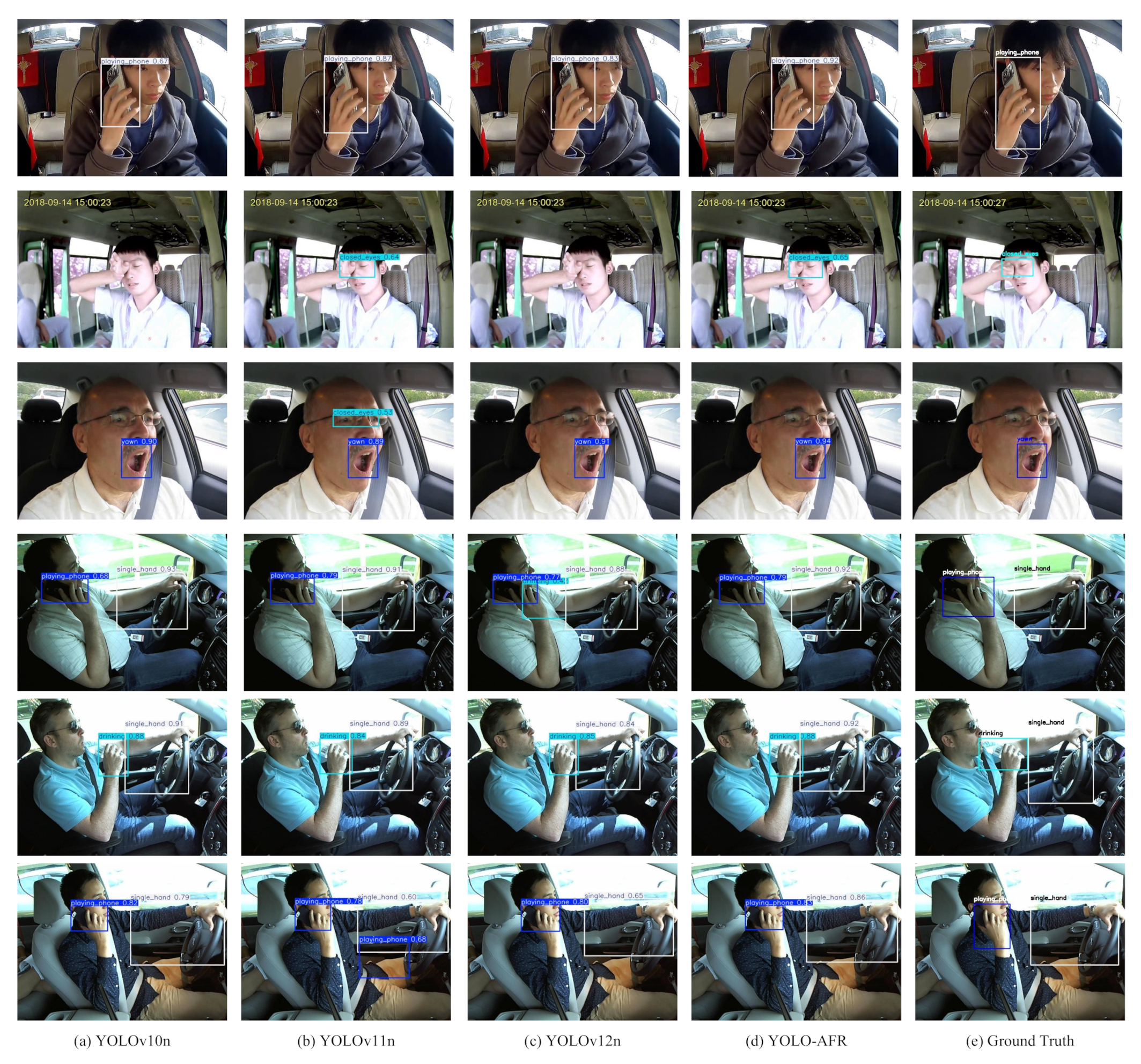
4.6. Visual Comparison of Detection Results

To qualitatively evaluate the detection performance of the proposed YOLO-AFR algorithm under real-world dangerous driving scenarios, we selected representative images containing six types of dangerous driving behaviors from the two datasets for testing. A comparative analysis was conducted against the baseline models YOLOv10n, YOLOv11n, and YOLOv12n, as illustrated in Figure 10.

As depicted in the figure, our improved YOLO-AFR model demonstrates superior performance, notably in reducing missed and false detections, which contributes to a significant enhancement in overall accuracy. Crucially, the benefits of this performance uplift become particularly evident when analyzing specific detection instances. While baseline models might achieve high overall accuracy, they can falter on certain challenging targets, resulting in lower precision for those particular detections. YOLO-AFR addresses this by substantially improving performance, specifically on these previously lower-accuracy targets. This targeted improvement, in turn, markedly boosts the credibility and reliability of the final detection results. Consequently, the reduction in detection errors (both missed and false detections), coupled with this enhanced overall credibility, clearly underscores the practical advantages of YOLO-AFR in real-world applications. These comprehensive enhancements are attributable to the strong environmental adaptability and robust occlusion-handling capabilities endowed by the integrated FRFN, SC-Conv, and SEAM modules. Collectively, these modules empower YOLO-AFR to accurately detect dangerous driving behaviors across various scales with heightened robustness and precision, even when faced with complex and challenging conditions.

4.7. In-Car Deployment Test

To further evaluate the real-time performance of the model, we deployed YOLO-AFR inside a vehicle and measured its frames per second (FPS). The deployment process is illustrated in Figure 11. A camera was installed within the vehicle to capture real-time footage of the driver. This footage was then transmitted to the model training server, which had the same configuration as our experimental environment, for real-time detection and output of results. The results indicated that our model achieved an average of 101.8 FPS during in-vehicle deployment, confirming its capability for real-time detection of dangerous driving behaviors.

5. Discussion

In terms of detection accuracy, as shown in Table 2 and Table 3, the proposed approach shows significant improvements in detecting small objects over traditional methods. Specifically, it achieves 0.976 and 0.989 mAP@0.5 on the YawDD-E and SfdDD public datasets, respectively. This represents an absolute improvement of 1.3 and 1.8 % in comparison with YOLOv12n (0.963 and 0.971). It also outperforms recent models such as YOLO-SGC (0.972 and 0.980), YOLOv10n (0.960 and 0.966), and YOLOv11n (0.963 and 0.972).

For practical deployment, the proposed model delivers competitive performance while maintaining computational feasibility. YOLO-AFR retains a compact model size with only 2.42 million parameters and 5.7 GFLOPs. This demonstrates a well-balanced trade-off between detection accuracy and model efficiency. The model achieves a processing speed of 104.59 FPS, significantly higher than recent baseline models and slightly lower than YOLO11n’s 123.21 FPS, yet still meets the real-time requirements of dangerous driving behavior detection under computational constraints.

Limitations

Despite these advances, YOLO-AFR has several limitations that warrant consideration. First, the improvement in detection accuracy for specific categories, such as “Single hand” in SfdDD and “Playing phone” in YawDD-E, is not significant enough. This indicates that while the newly integrated components enhance overall detection sensitivity, they can interfere with the model’s judgment for certain special categories, such as driving postures very similar to the normal state and tiny mobile phones. Therefore, the model’s generalization ability still needs to be strengthened. Second, although the current speed satisfies real-time needs, computational efficiency could be further improved without compromising accuracy. Lastly, the model does not currently incorporate driver gaze tracking, which limits its ability to make fine-grained assessments of vision-related dangerous driving behaviors.

6. Conclusions

This paper introduces an enhanced driver behavior detection model based on YOLOv12, named YOLO-AFR, to address the issue of existing dangerous driving behavior detection models struggling to achieve both accuracy and speed, thereby better tackling the prevalent problem of traffic safety. The model incorporates a Feature-Refinement Feedback Network (FRFN) to reconstruct the original A2C2f module in YOLOv12, forming a novel A2C2f-FRFN structure that enables adaptive optimization of multiscale features and significantly improves feature extraction in complex in-vehicle environments. A new C3k2_SC-Conv module is proposed, which integrates self-calibrated convolution (SC-Conv) into the C3k2 structure to extend the receptive field and elevate the accuracy of driver behavior detection. Additionally, the SEAM module is deployed in the detection head to boost global contextual awareness and prediction accuracy, effectively reducing missed and false detections in scenarios involving occlusions inside the vehicle.

Experimental results demonstrate that YOLO-AFR contains only 2.42 million parameters and 5.7 GFLOPs, achieving 0.976 and 0.989 mAP@0.5 on the YawDD-E and SfdDD datasets, respectively. This represents an absolute improvement of 1.3% and 1.8% compared to the baseline model YOLOv12n (0.963 and 0.971). It also outperforms recent models such as YOLO-SGC (0.972 and 0.980), YOLOv10n (0.960 and 0.966), and YOLOv11n (0.963 and 0.972). This confirms the model’s effectiveness in accurately detecting dangerous driving behaviors in complex environments. Furthermore, the model maintains real-time performance, with a processing speed of 104.59 FPS, significantly higher than recent baseline models and slightly lower than YOLO11n’s 123.21 FPS.

Future work will concentrate on several specific avenues. Firstly, to further enhance detection accuracy for challenging categories, particularly those involving high similarity to normal states or very small objects (e.g., “Single hand” driving, “Playing phone”), we will continue to refine attention mechanisms, optimize multiscale feature fusion strategies, investigate advanced loss functions, and adapt training methodologies. Secondly, to significantly improve computational efficiency for deployment on resource-constrained in-vehicle platforms, we will explore techniques such as quantization-aware training and network pruning to reduce model size and accelerate inference speed beyond the current 104.59 FPS. Thirdly, we will continue to research the deployment of the model in embedded systems to study its capabilities under performance constraints. Finally, a key direction will be the practical integration of the enhanced YOLO-AFR model into advanced driver assistance systems (ADAS). This will involve researching driver dangerous behavior recognition algorithms, such as by identifying combined behaviors, to better apply the object detection model in the field of practical traffic safety, thereby contributing more directly to on-road safety.

References

1. Ahmed, S.K.; Mohammed, M.G.; Abdulqadir, S.O.; El-Kader, R.G.A.; El-Shall, N.A.; Chandran, D.; Rehman, M.E.U.; Dhama, K. Road traffic accidental injuries and deaths: A neglected global health issue. Health Sci. Rep. 2023, 6, e1240. [Google Scholar] [CrossRef] [PubMed]
2. Singh, H.; Kushwaha, V.; Agarwal, A.D.; Sandhu, S.S. Fatal road traffic accidents: Causes and factors responsible. J. Indian Acad. Forensic Med. 2016, 38, 52–54. [Google Scholar] [CrossRef]
3. McManus, B.; Heaton, K.; Vance, D.E.; Stavrinos, D. The useful field of view assessment predicts simulated commercial motor vehicle driving safety. Traffic Inj. Prev. 2016, 17, 763–769. [Google Scholar] [CrossRef] [PubMed]
4. Piao, J.; McDonald, M. Advanced Driver Assistance Systems from Autonomous to Cooperative Approach. Transp. Rev. 2008, 28, 659–684. [Google Scholar] [CrossRef]
5. Hou, J.; Zhang, B.; Zhong, Y.; He, W. Research Progress of Dangerous Driving Behavior Recognition Methods Based on Deep Learning. World Electr. Veh. J. 2025, 16, 62. [Google Scholar] [CrossRef]
6. Song, W.; Zhang, G.; Long, Y. Identification of dangerous driving state based on lightweight deep learning model. Comput. Electr. Eng. 2023, 105, 108509. [Google Scholar] [CrossRef]
7. Negash, N.M.; Yang, J. Driver Behavior Modeling Toward Autonomous Vehicles: Comprehensive Review. IEEE Access 2023, 11, 22788–22821. [Google Scholar] [CrossRef]
8. Zakaria, N.J.; Shapiai, M.I.; Ghani, R.A.; Yassin, M.N.M.; Ibrahim, M.Z.; Wahid, N. Lane Detection in Autonomous Vehicles: A Systematic Review. IEEE Access 2023, 11, 3729–3765. [Google Scholar] [CrossRef]
9. Chen, L.W.; Chen, H.M. Driver Behavior Monitoring and Warning With Dangerous Driving Detection Based on the Internet of Vehicles. IEEE Trans. Intell. Transp. Syst. 2021, 22, 7232–7241. [Google Scholar] [CrossRef]
10. Jin, C.; Zhu, Z.; Bai, Y.; Jiang, G.; He, A. A Deep-Learning-Based Scheme for Detecting Driver Cell-Phone Use. IEEE Access 2020, 8, 18580–18589. [Google Scholar] [CrossRef]
11. Chien, T.C.; Lin, C.C.; Fan, C.P. Deep learning based driver smoking behavior detection for driving safety. J. Image Graph. 2020, 8, 15–20. [Google Scholar] [CrossRef]
12. Phan, A.C.; Trieu, T.N.; Phan, T.C. Driver drowsiness detection and smart alerting using deep learning and IoT. Internet Things 2023, 22, 100705. [Google Scholar] [CrossRef]
13. Jiang, H.; Learned-Miller, E. Face Detection with the Faster R-CNN. In Proceedings of the 2017 12th IEEE International Conference on Automatic Face & Gesture Recognition (FG 2017), Washington, DC, USA, 30 May–3 June 2017; pp. 650–657. [Google Scholar] [CrossRef]
14. Kehl, W.; Manhardt, F.; Tombari, F.; Ilic, S.; Navab, N. Ssd-6d: Making rgb-based 3d detection and 6d pose estimation great again. In Proceedings of the IEEE International Conference on Computer Vision, Venice, Italy, 22–29 October 2017; pp. 1521–1529. [Google Scholar]
15. Qin, X.; Yu, C.; Liu, B.; Zhang, Z. YOLO8-FASG: A High-Accuracy Fish Identification Method for Underwater Robotic System. IEEE Access 2024, 12, 73354–73362. [Google Scholar] [CrossRef]
16. Yu, C.; Yin, H.; Rong, C.; Zhao, J.; Liang, X.; Li, R.; Mo, X. YOLO-MRS: An efficient deep learning-based maritime object detection method for unmanned surface vehicles. Appl. Ocean Res. 2024, 153, 104240. [Google Scholar] [CrossRef]
17. Li, R.; Yu, C.; Qin, X.; An, X.; Zhao, J.; Chuai, W.; Liu, B. YOLO-SGC: A Dangerous Driving Behavior Detection Method With Multiscale Spatial-Channel Feature Aggregation. IEEE Sens. J. 2024, 24, 36044–36056. [Google Scholar] [CrossRef]
18. Zhang, R.; Liu, Y.; Wang, B.; Liu, D. CoP-YOLO: A Light-weight Dangerous Driving Behavior Detection Method. In Proceedings of the 2024 International Conference on Sensing, Measurement & Data Analytics in the Era of Artificial Intelligence (ICSMD), Huangshan, China, 31 October–3 November 2024; pp. 1–6. [Google Scholar] [CrossRef]
19. Zhou, S.; Chen, D.; Pan, J.; Shi, J.; Yang, J. Adapt or Perish: Adaptive Sparse Transformer with Attentive Feature Refinement for Image Restoration. In Proceedings of the IEEE/CVF Conference on Computer Vision and Pattern Recognition (CVPR), Seattle, WA, USA, 16–22 June 2024; pp. 2952–2963. [Google Scholar]
20. Liu, J.J.; Hou, Q.; Cheng, M.M.; Wang, C.; Feng, J. Improving Convolutional Networks With Self-Calibrated Convolutions. In Proceedings of the IEEE/CVF Conference on Computer Vision and Pattern Recognition (CVPR), Seattle, WA, USA, 13–19 June 2020. [Google Scholar]
21. Yu, Z.; Huang, H.; Chen, W.; Su, Y.; Liu, Y.; Wang, X. YOLO-FaceV2: A scale and occlusion aware face detector. Pattern Recognit. 2024, 155, 110714. [Google Scholar] [CrossRef]
22. Pomerleau, D. RALPH: Rapidly adapting lateral position handler. In Proceedings of the Intelligent Vehicles ’95. Symposium, Detroit, MI, USA, 25–26 September 1995; pp. 506–511. [Google Scholar] [CrossRef]
23. Gromer, M.; Salb, D.; Walzer, T.; Madrid, N.M.; Seepold, R. ECG sensor for detection of driver’s drowsiness. Procedia Comput. Sci. 2019, 159, 1938–1946. [Google Scholar] [CrossRef]
24. Tao, H.; Zhang, G.; Zhao, Y.; Zhou, Y. Real-time driver fatigue detection based on face alignment. In Proceedings of the Ninth International Conference on Digital Image Processing (ICDIP 2017), Hong Kong, China, 19–22 May 2017; Volume 10420, p. 1042003. [Google Scholar] [CrossRef]
25. Girshick, R.; Donahue, J.; Darrell, T.; Malik, J. Rich Feature Hierarchies for Accurate Object Detection and Semantic Segmentation. In Proceedings of the IEEE Conference on Computer Vision and Pattern Recognition (CVPR), Columbus, OH, USA, 23–28 June 2014. [Google Scholar]
26. Liu, W.; Anguelov, D.; Erhan, D.; Szegedy, C.; Reed, S.; Fu, C.Y.; Berg, A.C. SSD: Single Shot MultiBox Detector. In Proceedings of the Computer Vision—ECCV 2016; Leibe, B., Matas, J., Sebe, N., Welling, M., Eds.; Springer: Cham, Switzerland, 2016; pp. 21–37. [Google Scholar]
27. Redmon, J.; Farhadi, A. Yolov3: An incremental improvement. arXiv 2018, arXiv:1804.02767. [Google Scholar]
28. Jocher, G.; Stoken, A.; Borovec, J.; Changyu, L.; Hogan, A.; Diaconu, L.; Poznanski, J.; Yu, L.; Rai, P.; Ferriday, R.; et al. ultralytics/yolov5: V3.0. Zenodo. 2020. Available online: https://zenodo.org/records/3983579 (accessed on 23 May 2025).
29. Li, C.; Li, L.; Geng, Y.; Jiang, H.; Cheng, M.; Zhang, B.; Ke, Z.; Xu, X.; Chu, X. YOLOv6 v3.0: A Full-Scale Reloading. arXiv 2023, arXiv:2301.05586. [Google Scholar]
30. Wang, C.Y.; Bochkovskiy, A.; Liao, H.Y.M. YOLOv7: Trainable Bag-of-Freebies Sets New State-of-the-Art for Real-Time Object Detectors. In Proceedings of the IEEE/CVF Conference on Computer Vision and Pattern Recognition (CVPR), Vancouver, BC, Canada, 17–24 June 2023; pp. 7464–7475. [Google Scholar]
31. Sohan, M.; Sai Ram, T.; Rami Reddy, C.V. A Review on YOLOv8 and Its Advancements. In Proceedings of the Data Intelligence and Cognitive Informatics; Jacob, I.J., Piramuthu, S., Falkowski-Gilski, P., Eds.; Springer: Singapore, 2024; pp. 529–545. [Google Scholar]
32. Wang, C.Y.; Liao, H.Y.M. YOLOv9: Learning What You Want to Learn Using Programmable Gradient Information. arXiv 2024, arXiv:2402.13616. [Google Scholar]
33. Wang, A.; Chen, H.; Liu, L.; Chen, K.; Lin, Z.; Han, J.; Ding, G. YOLOv10: Real-Time End-to-End Object Detection. arXiv 2024, arXiv:2405.14458. [Google Scholar]
34. Khanam, R.; Hussain, M. YOLOv11: An Overview of the Key Architectural Enhancements. arXiv 2024, arXiv:2410.17725. [Google Scholar]
35. Tian, Y.; Ye, Q.; Doermann, D. YOLOv12: Attention-Centric Real-Time Object Detectors. arXiv 2025, arXiv:2502.12524. [Google Scholar]
36. Le, T.N.; Ono, S.; Sugimoto, A.; Kawasaki, H. Attention R-CNN for Accident Detection. In Proceedings of the 2020 IEEE Intelligent Vehicles Symposium (IV), Las Vegas, NV, USA, 19 October–13 November 2020; pp. 313–320. [Google Scholar] [CrossRef]
37. Yang, T.; Yang, J.; Meng, J. Driver’s Illegal Driving Behavior Detection with SSD Approach. In Proceedings of the 2021 IEEE 2nd International Conference on Pattern Recognition and Machine Learning (PRML), Chengdu, China, 16–18 July 2021; pp. 109–114. [Google Scholar] [CrossRef]
38. Amira, B.G.; Zoulikha, M.M.; Hector, P. Driver drowsiness detection and tracking based on YOLO with Haar cascades and ERNN. Int. J. Saf. Secur. Eng. 2021, 11, 35–42. [Google Scholar] [CrossRef]
39. Trockman, A.; Kolter, J.Z. Patches Are All You Need? arXiv 2022, arXiv:2201.09792. [Google Scholar]
40. Abtahi, S.; Omidyeganeh, M.; Shirmohammadi, S.; Hariri, B. YawDD: Yawning Detection Dataset. 2020. Available online: https://ieee-dataport.org/open-access/yawdd-yawning-detection-dataset (accessed on 23 May 2025). [CrossRef]
41. yunxizhineng. VOC-COCO Dataset. Available online: https://aistudio.baidu.com/datasetdetail/94583/0 (accessed on 23 May 2025).
42. Barcelona Autonomous University, Computer Vision Center. CVC11 DrivFace Dataset. Available online: https://archive.ics.uci.edu/dataset/378/drivface (accessed on 23 May 2025).
43. Montoya, A. State Farm Distracted Driver Detection. Available online: https://www.kaggle.com/competitions/state-farm-distracted-driver-detection/data (accessed on 23 May 2025).
44. Ren, S.; He, K.; Girshick, R.; Sun, J. Faster R-CNN: Towards Real-Time Object Detection with Region Proposal Networks. IEEE Trans. Pattern Anal. Mach. Intell. 2017, 39, 1137–1149. [Google Scholar] [CrossRef]
45. Narayanan, A.; Kaimal, R.M.; Bijlani, K. Yaw Estimation Using Cylindrical and Ellipsoidal Face Models. IEEE Trans. Intell. Transp. Syst. 2014, 15, 2308–2320. [Google Scholar] [CrossRef]
46. Yang, H.; Liu, L.; Min, W.; Yang, X.; Xiong, X. Driver Yawning Detection Based on Subtle Facial Action Recognition. IEEE Trans. Multimed. 2021, 23, 572–583. [Google Scholar] [CrossRef]
47. Kır Savaş, B.; Becerikli, Y. Behavior-based driver fatigue detection system with deep belief network. Neural Comput. Appl. 2022, 34, 14053–14065. [Google Scholar] [CrossRef]
48. Dong, B.T.; Lin, H.Y.; Chang, C.C. Driver Fatigue and Distracted Driving Detection Using Random Forest and Convolutional Neural Network. Appl. Sci. 2022, 12, 8674. [Google Scholar] [CrossRef]
49. Bai, J.; Yu, W.; Xiao, Z.; Havyarimana, V.; Regan, A.C.; Jiang, H.; Jiao, L. Two-Stream Spatial–Temporal Graph Convolutional Networks for Driver Drowsiness Detection. IEEE Trans. Cybern. 2022, 52, 13821–13833. [Google Scholar] [CrossRef] [PubMed]
50. Alameen, S.A.; Alhothali, A.M. A Lightweight Driver Drowsiness Detection System Using 3DCNN With LSTM. Comput. Syst. Sci. Eng. 2023, 44, 895. [Google Scholar] [CrossRef]
51. Li, A.; Ma, X.; Guo, J.; Zhang, J.; Wang, J.; Zhao, K.; Li, Y. Driver fatigue detection and human-machine cooperative decision-making for road scenarios. Multimed. Tools Appl. 2024, 83, 12487–12518. [Google Scholar] [CrossRef]
52. Abouelnaga, Y.; Eraqi, H.M.; Moustafa, M.N. Real-time Distracted Driver Posture Classification. arXiv 2018, arXiv:1706.09498. [Google Scholar]
53. Baheti, B.; Talbar, S.; Gajre, S. Towards Computationally Efficient and Realtime Distracted Driver Detection with MobileVGG Network. IEEE Trans. Intell. Veh. 2020, 5, 565–574. [Google Scholar] [CrossRef]
54. Qin, B.; Qian, J.; Xin, Y.; Liu, B.; Dong, Y. Distracted Driver Detection Based on a CNN with Decreasing Filter Size. IEEE Trans. Intell. Transp. Syst. 2022, 23, 6922–6933. [Google Scholar] [CrossRef]
55. Li, W.; Wang, J.; Ren, T.; Li, F.; Zhang, J.; Wu, Z. Learning Accurate, Speedy, Lightweight CNNs via Instance-Specific Multi-Teacher Knowledge Distillation for Distracted Driver Posture Identification. IEEE Trans. Intell. Transp. Syst. 2022, 23, 17922–17935. [Google Scholar] [CrossRef]
56. Shang, E.; Liu, H.; Yang, Z.; Du, J.; Ge, Y. FedBiKD: Federated Bidirectional Knowledge Distillation for Distracted Driving Detection. IEEE Internet Things J. 2023, 10, 11643–11654. [Google Scholar] [CrossRef]
57. Gao, H.; Liu, Y. Improving real-time driver distraction detection via constrained attention mechanism. Eng. Appl. Artif. Intell. 2024, 128, 107408. [Google Scholar] [CrossRef]
58. Chillakuru, P.; Ananthajothi, K.; Divya, D. Three stage classification framework with ranking scheme for distracted driver detection using heuristic-assisted strategy. Knowl.-Based Syst. 2024, 293, 111589. [Google Scholar] [CrossRef]
Figure 1. Structure of YOLO-AFR Network. *n indicates that the module is repeated n times within the overall architecture. *2 indicates that the module is configured to execute sequentially in pairs. *C2_weight refers to multiplying a result by channel weights.
Applsci 15 06090 g001
Figure 2. Structure of YOLOv12 Network.
Applsci 15 06090 g002
Figure 3. Structure of Feature-Refinement Feedforward Network(FRFN).
Applsci 15 06090 g003
Figure 4. Structure of SC-Conv.
Applsci 15 06090 g004
Figure 5. Structure of Separated and Enhancement Attention Module (SEAM).
Applsci 15 06090 g005
Figure 6. Sample display of the YawDD-E and SfdDD datasets.
Applsci 15 06090 g006
Figure 7. Our YOLO-AFR is compared with other real-time detectors in terms of accuracy and speed on the SfdDD dataset. The radius of the circle represents GFLOPs.
Applsci 15 06090 g007
Figure 8. mAP@0.5 Gains for Method Combinations on SfdDD and YawDD-E Datasets.
Applsci 15 06090 g008
Figure 9. Synergistic Interaction of FRFN, SC-Conv, and SEAM.
Applsci 15 06090 g009
Figure 10. Qualitative Comparison of Detection Results on Real-World Dangerous Driving Scenarios.
Applsci 15 06090 g010
Figure 11. In-Car Model Deployment Architecture.
Applsci 15 06090 g011