Abstract
This study presents a seismic tomography analysis of the Târgu Jiu region in southwestern Romania, an area that experienced an unusual earthquake sequence in 2023. Using P- and S-wave arrival times local earthquakes, we applied the LOTOS algorithm to produce high-resolution 3D crustal seismic velocities models. High Vp and Vs values in the northern and northeastern areas suggest the presence of dense, rigid geological formations, likely associated with consolidated magmatic or metamorphic units. In contrast, the central region exhibits low Vs values, coinciding with an active seismic zone and intersecting major fault structures. This suggests the presence of highly fractured and weakly consolidated rocks, potentially saturated with fluids. The Vp/Vs ratio in the central region reached values of ≥1.8–1.9, indicating fluid-filled fractures that may influence fault dynamics and earthquake occurrence. In the southern region, velocity anomalies suggest weakly consolidated sedimentary units with a high degree of fracturing. These findings contribute to a better understanding of the geodynamic behavior of the Târgu Jiu area and its seismic hazard potential.
1. Introduction
Târgu Jiu is located in the southwestern part of Romania, close to the contact of Getic Depression with the South Carpathians (Figure 1). The South Carpathians is one of the most twisted segments of the Alpine orogen where the orientation of the orogen range suddenly shifts from east–west to north–south, and then turns back to east–west toward the Balkans. The present-day configuration of the South Carpathians system is the result of a long evolution that includes multiple tectonic processes like: plate convergence and collision, lithospheric stretching and break-up, orogen-parallel extension, rotation and wrenching and basin opening and inversion [1,2].
The Getic foreland basin (Figure 1) is located along the northern edge of the Moesian Plate, within the Getic Depression, and is composed of Neogene sediments that reach thicknesses of up to 3000 m [3]. The Getic Depression is well-known as a hilly region connecting the Moesian Platform with the South Carpathians. It extends between the Dâmbovița River in the east and the Danube Valley in the west, with its southern boundary marked by the Pericarpathian Fault. The Getic Depression was formed as a result of large-scale transcurrent movements generated by the Paleogene to Early Miocene displacement and clockwise rotation of the Tisza–Dacia Unit around the western Moesia corner, followed by the Badenian–Sarmatian uplift of the South Carpathian units [4,5]. The Getic Depression initially formed in the Late Paleogene-Early Miocene as a pull-apart basin, with its development controlled by the Timok–Cerna Jiu fault system [6]. Later, during the Sarmatian tectonic event, the pre-existing E–W fault system was inverted by an oblique compression generated by the eastward movement of the Tisza–Dacia tectonic block [7].
The tectonic molding around the Moesian platform of the South Carpathians observed west of Târgu Jiu began in the Oligocene and was mostly shaped by dextral wrenching along the Cerna Fault [8]. The dextral wrenching continued into the Early Miocene, but more externally along the Timok Fault, with a dextral displacement of 65 km. In the Middle Miocene, dextral faults cut in the E–W and NW–SE direction the sedimentary cover of the Getic Depression [2,9]. Beneath the sedimentary cover of the Getic depression and in the area lined up in the extension of the Timok Fault, a perpendicular normal fault system is found along the western edge of the Moesian Platform. The N–S fault system originates from the Permo-Triassic rift and a younger E–W normal fault system mostly formed during the Mid-Tertiary period [2].
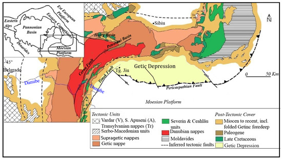
Figure 1.
Tectonic framework of the Getic Depression in relation to Carpathian orogen and the Moesian Platform (modified after [10]) and location of the study area (Târgu Jiu).
The area around Târgu Jiu city has been considered until 2023 an area of low seismic activity, not included in the seismogenic zones of Romania. Seismic activity in the Getic Depression (Figure 1) is generally manifested by earthquakes of moderate size, rarely exceeding magnitude Mw = 5 [11]. The most significant earthquakes before 2023 were recorded on 20 June 1943 (Mw = 5.2) produced east of Tismana, on 9 July 1912 (Mw = 4.5) about 9 km south of Târgu Jiu, and on 4 May 1963 (Mw = 4.5), about 22 km NW of the same location. However, since February 2023, the area has experienced a significant intensification of seismic activity, highlighting more complex seismotectonic processes than initially thought. The earthquake sequence that started in February 2023 outlines a notable potential to generate significant earthquakes and draws attention of the scientific community to the complex tectonic mechanisms that are still active at present in this area [12,13,14]. Recent events underline the need for in-depth research to better understand the tectonic dynamics and adequately prepare for seismic hazards. Of note, the Getic Depression is a geological unit characterized by the presence of sedimentary formations favorable for the accumulation of hydrocarbons, and the first exploration and drilling activities for hydrocarbon extraction in this area started in the 1960s. Considering these particularities, the need to know in detail the geological structure in correlation with the geodynamics of the area becomes increasingly a demanding issue with implications on seismic hazard assessment.
One tool that has proven to be particularly useful for investigating the 3D internal structure of the Earth is the seismic tomography. It inverts the structural model in a given area according to how seismic waves passing through it vary across that area. Both body waves and surface waves generated by earthquakes or explosions and seismic noise can be used in an inversion. It provides information about seismic wave velocity variations. Thus, areas with low velocities indicate warm, weakly consolidated or fluid-rich regions, such as magmatic chambers or active faults, and areas with high velocities reflect cold, rigid regions, such as stable lithospheric blocks or dense rocks.
Seismic tomography has been widely applied both on global and local scales. For example, the application of seismic tomographic imaging techniques at the European scale provided spectacular 3D images of mantle structures which can readily be linked to global plate tectonic processes, such as the past and active subduction of lithospheric plates [15,16], mantle plumes originating at a great depth [17,18,19,20], and related surface processes such as intra-plate volcanism, rifting and vertical surface motions. Tomographic images contributed essentially to understanding and modelling of the coupled mantle–surface processes, a major research direction developed within the TOPO EUROPE initiative [21].
Tomography studies for the Carpathian–Pannonian region were developed following the installation of temporary stations first using teleseismic data (CALIXTO experiment, South Carpathian Project, 2009–2011) [22,23,24] and then, ambient noise data [25,26]. To date, only one study has used local earthquake data for tomographic inversion focused on the Vrancea seismic region [27]. A number of features are common to all these investigations: the presence of a high-velocity body localized quasi-vertically beneath the Vrancea zone below 60 km depth and co-located with the intermediate-depth earthquake source, the diapiric upwelling of asthenospheric mantle (crustal thinning) on the one hand and the descent of a remnant subducted slab beneath Pannonian Basin in the mantle transition zone (400–600 km) on the other hand.
The aim of this study was to show the seismic tomography of the Târgu Jiu region using P- and S-wave arrivals from local events, to characterize its crustal structure through tomographic studies and to identify potential zones of geological hazard through seismological studies. Unlike the Vrancea area located in the bending zone of the Eastern Carpathians, the target area investigated in our study is characterized by moderate and less frequent inland seismicity located in the crust. However, the intensification of seismic activity recorded in 2023 has increased the interest in this area, both from the point of view of geodynamic modeling and updating the associated seismic hazard.
2. Data and Methodology of Inversion
2.1. Data Description
The Târgu Jiu earthquake sequences have their epicenters located in a distinctive area at the interface between the South Carpathian curvature and the Getic Depression (South Carpathian Foredeep). The seismic sequence of 2023 began on 13 February with a significant double shock of magnitudes Mw = 4.8 and Mw = 5.4, followed by over 4000 aftershocks, with magnitudes ranging from 1.1 to 4.6 [12,13,14]. Considering that the layout of the seismic network during the seismic sequence was not the most suitable for a seismic tomography study, the dataset was extended with more than 1000 seismic events that occurred in the regions surrounding the studied area recorded since 2016. The dataset used in the study consists of 5323 earthquakes (see Figure 2) that occurred in the Târgu Jiu region and its surroundings from 2016 until December 2023. More than 3900 earthquakes are derived from the seismic sequence that started on 13 February 2023, in the northwest part of Târgu Jiu.
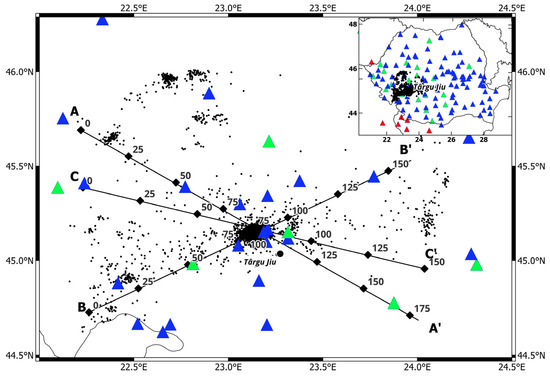
Figure 2.
Location of seismic events and vertical sections used for seismic tomography in the study region. Black dots are the events. Colored triangles are seismic stations (blue for RSN, green for AdriaArray and red for outside the border stations).
The initial locations were performed using the LocSAT [28] algorithm embedded within the Antelope v5.14 software [29], which is operated by the National Institute for Earth Physics (NIEP) for routine earthquake locations. A total number of 108,016 picks with 51,598 P-data and 56,418 S-data from 133 seismic stations (Figure 2) were processed. The Romanian Seismic Network (RSN) [30] operated by the NIEP, designed to monitor and analyze the seismicity of Romania, covers the entire country surface with an average density of 30 km inter-station distance. The RSN’s capabilities are further strengthened by collaboration protocols with neighboring countries, allowing for NIEP to acquire and archive seismic data from additional seismic stations located outside Romania [31]. This cross-border integration enhances the network’s ability to detect and analyze borders or regional seismic events. At present, NIEP is an EIDA (European Integrated Data Archive) node collecting, archiving and providing data for the neighboring countries: ”https://www.orfeus-eu.org/data/eida/nodes/NIEP/ (accessed on 21 May 2025)”. Most of the seismic stations selected for our study, shown in Figure 3, are part of the RSN. Some stations belong to the AdriaArray project [32] which aimed to investigate the entire Adriatic plate in southeastern Europe by covering the area with a dense temporary seismic network.
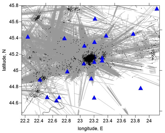
Figure 3.
Map view of ray coverage for P-waves within the 12.5–17.5 km depth range. Black dots are the events, blue triangles are the seismic stations and the gray lines are P-wave ray paths.
All these events have been reviewed and included in the ROMPLUS earthquake catalog [33,34], respecting localization quality criteria such as RMS < 1 s or GAP < 120, where GAP represents the maximum azimuthal gap between stations surrounding an event, used to evaluate the reliability of its location. For the tomographic inversion, we applied additional criteria to select the input dataset: at least 6 picks per event and the absolute values of residuals after source location in the 1D model should not exceed 0.7 s. The final dataset consists of 105,976 arrival times from 5281 events with 50,533 P-wave and 55,443 S-wave arrival times. Figure 3 shows the ray coverage of the dataset.
2.2. Tomographic Inversion
The tomographic inversion was performed using the LOTOS code for body wave tomography and passive sources [35]. This code has also been applied in several studies on seismic areas in Romania [27,36,37], as well as on regions worldwide where, among seismicity, volcanoes have been studied [38,39,40,41,42]. The calculation procedure begins with the absolute location of the sources within the reference 1D velocity model, using a grid search method to determine the optimal coordinates of the events. At this stage, travel times are calculated in a simplified manner along straight lines using the 1D velocity distributions. In the next stage, the sources are relocated using a more precise algorithm based on the 3D ray-bending method initially proposed by [43]. The velocity model was parameterized using a set of nodes distributed throughout the study volume, depending on ray coverage. Horizontally, these nodes were distributed regularly with a constant spacing of 5 km only in areas with sufficient ray coverage (see Figure 4), while vertically, the distance between nodes was set to 2 km. To minimize potential artefacts related to the node geometry, the LOTOS code allows for performing the inversion using four grids with different baseline azimuths for node distribution (i.e., 0°, 22°, 45°, and 67°). After computing the models for all grids, they were averaged and merged into a regular spacing model, which was then used in the next iteration for source relocation. In total, we stopped at five iterations as a compromise between computational cost and minimizing nonlinear effects.
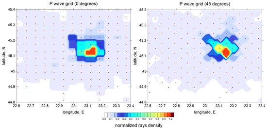
Figure 4.
Distributions of nodes of two parameterization P-wave grids (red dots) with different basic orientations (0 degrees, left and 45 degrees, right) used for the inversions. The background is the normalized ray density in the depth range 12.5–17.5 km.
The inversion was performed using the least squares with QR decomposition (LSQR) [44,45]. Its stability was controlled by amplitude damping and flattening regularization which was defined from synthetic modeling as giving the best recovery of known structures. To determine the most appropriate regularization coefficients (damping and smoothing), we performed a series of inversions with systematically varied parameters. We evaluated each combination in terms of the residual RMS reduction, the sharpness of the anomalies in the tomographic model, and the ability to recover synthetic anomalies by a checkerboard test. The optimal value was considered the one that provided the best compromise between fidelity to the data and geologic stability of the model. In our case, the regularization coefficients were amplitude damping and flattening of 4 and 7 for P- and S-wave models.
2.3. Data Testing
To evaluate the random noise in the data, we performed an odd/even test in which we also evaluated the stability of the 1D model. Then, we compared the inversion results obtained with the same parameters. If the images are very different, it may indicate problems in the data or in the reconstruction algorithm. In our case, the results of the odd/even test for the P- and S-wave velocity anomalies at 15 km depth are presented in Figure 5 and a good correlation of the structures can be observed.
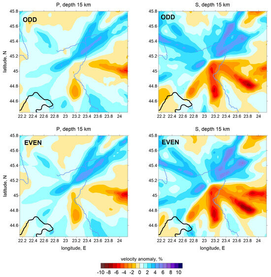
Figure 5.
Odd/even events test (black line is the border line and the blue lines are rivers).
The spatial resolution of the model was evaluated by synthetic tests in which we reproduced the same processing conditions of the experimental data. To define the modeling rays, we used the same source–receiver pairs as in the experimental dataset, with the event locations taken from the final solution of the main model. The synthetic model was built by overlaying a set of 3D anomalies on a 1D reference model. Synthetic travel times were computed in the 3D model using a ray-tracing bending algorithm. To simulate realistic conditions, we introduced random noise with predefined standard deviations of 0.1 and 0.2 for the P-wave and S-wave data, respectively. These noise levels were selected to achieve a variance reduction comparable to that of inverting experimental data. The number of iterations and all control parameters during the synthetic model recovery were identical to those used to compute the main model. To optimize the recovery quality, we adjusted the control parameters during the synthetic tests and then applied these optimal values to the inversion of the experimental data in the main model. This process involved running the synthetic modeling and the experimental data inversion concurrently.
Figure 6 shows the results of a checkerboard test in which the synthetic anomalies were represented as 40 × 40 × 20 km. Within these cubes, alternating anomalies with amplitudes of ±5% were introduced. For dVp and dVs, anomalies were assigned opposite signs to enhance the contrast of the Vp/Vs ratio. The inversion of the P- and S-wave data produced a variance reduction of about 55% and 50% for the P- and S-wave data, compared to those of the inversion of the experimental data, respectively, 40% for P and 54% for S, which shows a more accurate model than the original one. The recovered results in Figure 6 are displayed in three depth sections, corresponding to the central regions of the anomalies in different layers. The results show that in the first two layers, the recovered anomaly amplitudes are close to the original values for both P- and S-waves. However, in the deepest layer, the P-wave amplitudes appear slightly smaller. This suggests that a single set of damping parameters may not achieve optimal amplitude recovery across the entire survey volume. Increasing the damping to enhance recovery in deeper sections can result in amplitude loss in shallower regions, potentially obscuring important anomalies. To balance this, the damping value was selected to maintain the stability of anomaly shapes while minimizing noise artifacts. Features smaller than ~40 km laterally and ~20 km vertically were not considered reliably resolvable in our dataset.
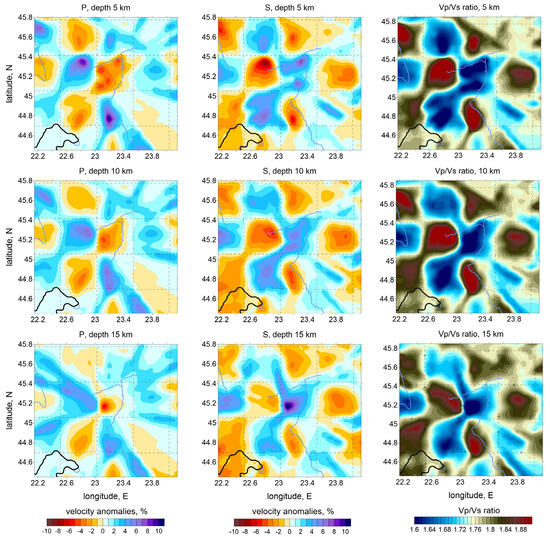
Figure 6.
Checkerboard test to assess the spatial resolution. The anomalies are defined in cubes of 40 × 40 × 20 km. The recovered results for the dVp, dVs, and Vp/Vs ratio are shown in three horizontal sections. The shapes of the synthetic anomalies are highlighted with dotted lines (black line is the border line and the blue lines are rivers).
To estimate the vertical resolution, we performed a synthetic test with anomalies defined along the vertical profiles. Typically, the vertical resolution is weaker than the horizontal resolution due to the trade-off between source depth and velocity distribution in tomography studies. Figure 7 shows the vertical checkerboard P-wave vertical tests associated with the vertical profiles used to present the main results. In the horizontal direction, the anomalies were defined with a size of 40 km, and in the vertical direction, the anomaly signs changed at a 20 km depth. The section thickness was 30 km. Model reconstruction was good, especially in regions with sources and ray intersections.
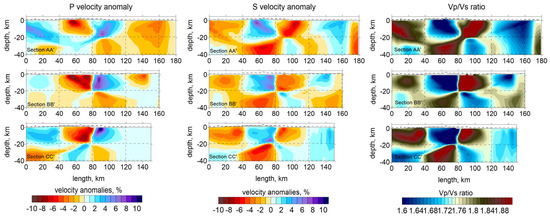
Figure 7.
Vertical checkerboard test.
The recovered event locations from the synthetic test are presented in Figure 8. These were compared with their input values, and the average relocation errors after the final iteration were found to be 1.18 km, which is within one grid cell dimension. This confirms that the inversion process does not significantly distort the positions of the events.
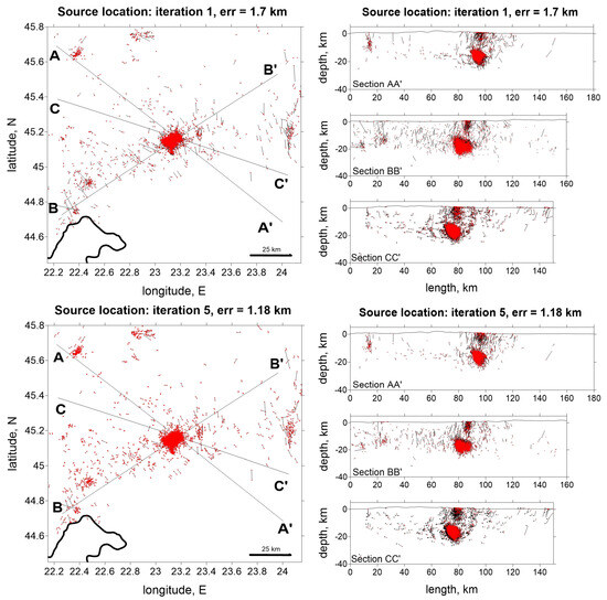
Figure 8.
Event locations presented in map view (left) and cross sections (right) through the checkerboard test presented in Figure 6 after one (top) and five (bottom) iteration(s). Red dots are the resulting locations; bars are the mean errors with respect to the initial locations. The configuration of the vertical cross sections is indicated in the left map.
We performed an additional set of resolution tests using realistic synthetic anomalies in Figure 9. In the P-wave model, two anomalies were introduced with amplitudes of −3% and −6%. For the S-wave model, the anomalies shared the same shapes as those in the P-wave model, but had different amplitudes of −6% and −8%. The inversion results showed that the damped values of the anomalies were retrieved within the initial anomaly limits P.
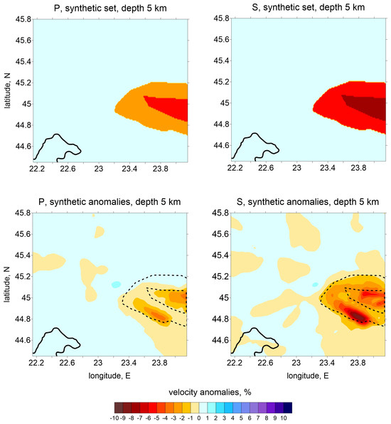
Figure 9.
Synthetic test with free-shaped anomalies defined in the horizontal projection. Upper row presents the initial synthetic models for the P- and S-wave velocity anomalies. Lower row shows the recovered anomalies. The shapes of the initial anomalies are highlighted with dotted lines.
3. Results
3.1. 1D Model Optimization
Data processing starts with preliminary source localization and 1D model optimization. The best 1D model that describes our dataset was determined using several starting velocity models (Figure 10A). We tested several 1D models previously developed by [4] (model 2), [46] (model 3) or [47] (model 4), and we also developed a model (model 1) based on our data using the VELEST code [48]. Figure 10A shows the starting models and their optimizations, and Table 1 shows the RMS residuals after the first and fifth iterations.
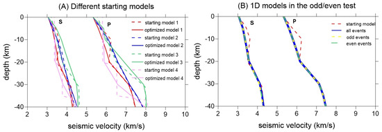
Figure 10.
Optimization of the 1D model for observed data. (A) Optimization results with observed data and different starting 1D models. Different colors indicate different models, dotted lines are starting models and bold lines of corresponding colors are the optimization results. (B) Optimization results for halved data subsets in the odd/even test.

Table 1.
RMS values for P- and S-wave residuals after the first and fifth iterations for different starting models.
The process for obtaining the 1D minimum velocity model for the Târgu–Jiu region started with the selection of the initial realistic velocity models already tested for the western part of Romania [13,36,46,49]. The concept of the 1D minimum velocity model involves several parameters such as station corrections, reference station and velocity. Station corrections play an essential role in improving the accuracy and reliability of subsequent 3D tomographic inversion. As recommended in previous studies [48,50], the VELEST algorithm is typically employed to initiate the 1D inversion using a stratified model with numerous shallow layers. These layers are later combined during the iterative inversion process as velocity values converge, ensuring a stable and representative starting model for 3D tomography. The 1D minimum velocity model is obtained from the inversion of the arrival times recorded at the station for each event.
Analyzing the values of the RMS residuals presented in Table 1, we concluded that the most likely 1D model for our data is model 1, presented in Table 2. The stability of the model was assessed by the “odd/even” test [51]. The test consists of running inversions on subsets of the data obtained by separating events with even and odd identification numbers. The starting model for the odd and even subsets of data and for the entire dataset is the same and corresponds to model 1 in Figure 10A. The optimization results are similar for all cases and are shown in Figure 10B. This test reveals that the dataset does not affect the stability of the 1D model optimization.
Table 2.
P- and S-velocities in the reference 1D model after optimization.
As shown in Figure 10, the model 4 [47], which is a global model, greatly underestimated the velocity values over the entire depth range and for this reason deviates the 1D model obtained by inversion toward low values. On the contrary, the model proposed by [46] (model 3) for the intra-Carpathian area overestimated the velocities, especially for larger depths (below 10 km). The most suitable models were located between these two extremes (models 1 and 2). We note that model 2 varies quasi-continuously with depth (no jumps in the velocity).
3.2. Relocated Seismicity
Figure 11 shows the distribution of relocated seismicity with the LOTOS algorithm. In general, the relocated hypocentral depths were slightly larger compared to the original depths from ROMPLUS Catalog [33,34]. Several clusters of earthquakes were observed at the extremities of the map (left), as well as the cluster of events from the center of the map associated with the Târgu Jiu earthquake sequence. Vertical sections (right) show the relocated hypocenters corresponding to the marked profiles. Depths are given in km. Most seismicity is concentrated between 5 and 25 km depth, with a dominant cluster around 15–25 km. There is also a correlation of the earthquakes with the fault paths in the area; the main cluster in the center seems to have a NE–SW orientation.
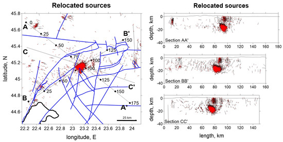
Figure 11.
LOTOS relocated seismicity. Red dots are the resulting locations, bars are the mean errors with respect to the initial locations, blue lines are fault lines. Locations of the vertical cross sections are indicated in the left-side map.
3.3. P and S Wave Velocity Anomalies
The main tomography results are the 3D models of P- and S-wave velocity models from a five-iteration inversion used to generate tomographic images, a compromise between computation time and the quality of the solution (nonlinear effect reduction). Table 3 shows the RMS residuals reduction after iterations for the reference 1D model. Figure 12 presents the results for P and S anomalies in horizontal slices at depths of 5, 10, 15 and 20 km and Figure 13 shows the anomalies for P- and S-wave and Vp/Vs ratio in three vertical sections passing through the study area. The P- and S-wave velocity anomalies are expressed as percentage deviations from the optimized 1D reference velocity model. The Vp/Vs ratio was computed by dividing the derived absolute velocities of Vp by Vs.
Table 3.
The RMS residuals reduction for the reference 1D model.
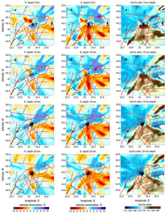
Figure 12.
P- and S-wave velocity anomalies in horizontal slices, in percent with respect to the optimized 1D velocity model. Black dots depict the relocated sources around the corresponding depth levels, and the main faults are presented with red lines.
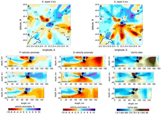
Figure 13.
P wave velocity anomalies in vertical sections (left), S wave velocity anomalies (middle) and Vp/Vs ratio (right). The locations of the profiles are shown on top in the horizontal section for P and S. Dots indicate the relocated sources at distances less than 20 km from the profile. Blue triangles are seismic stations, black line is the border line and blue line are rivers.
The P- and S-wave velocity structure shows a strong correlation in both horizontal slices and vertical cross-sections. The Vp/Vs ratio cross-sections (Figure 13) reveal structural patterns consistent with those observed in the primary P-wave models. The independently derived P- and S-wave models exhibit similar features, supporting the reliability of the inversion results and indicating that the available dataset is adequate for confidently resolving the identified structure.
4. Discussion
Analyzing the distribution of P-wave (Vp) and S-wave (Vs) velocities, distinct geophysical properties can be identified. First, a general NE–SW trend which separates two regions of contrast in velocity. The regions in the north and northeast of the maps, with high Vp and Vs values, indicate the presence of denser and more rigid rocks, possibly associated with consolidated geological units such as magmatic rock masses or closed and inactive faults. Areas with low Vp values may indicate the presence of less consolidated rocks, areas of intense fracturing, or the presence of fluids (groundwater, magmatic fluids, or gases). The NE–SW alignment crossing the epicentral area of the sequence of 2023 suggests the presence of an active fault oriented along this alignment.
A significant low Vs anomaly overlaps with the central area of the map, where multiple earthquakes are located, suggesting the presence of weakly consolidated rocks with intense fracturing, as also observed in the representation of the main faults in the area (according to Project: CEEX Project No. 647/2005, Map of the Main Fault Systems in Romania). These negative anomalies also extend to the south and southeast to the Getic Depression, which is a sedimentary basin filled with 4–5 km of Paleozoic units [52]. These units consist of loose formations with lower seismic velocities compared to the older and well-compacted Danubian units to the north. Seismic waves propagate more slowly through sedimentary formations [53], but surface waves can be significantly amplified [54]. This amplification effect increases the potential for destruction, as surface waves tend to cause more damage to buildings and infrastructure. Moreover, the numerous faults that cross the Getic Depression in a W–E direction represent a secondary factor that justifies the slow seismic velocities in this sedimentary basin.
The finger-like shape of the anomalies (the shape of a three-fingered hand) visible in Figure 12 is reflecting an artificial modulation of the distribution of the anomalies due to the uneven ray coverage (the fact that the events are tightly clustered in the center and the stations are distributed over a large area giving a radial system of rays that does not provide sufficient ray intersections (see Figure 3)).
S-wave velocities are more sensitive to the presence of fluids, so their decrease in these regions may indicate the presence of fluids in crustal fissures. The Vp/Vs ratio in the central area is high, with values ≥1.8–1.9, which may suggest the presence of fluids in fractured rocks, contributing to a stronger decrease in S-wave velocity than in P-wave velocity. According to Figure 12, this area matches with the seismically active region, suggesting that fluids [55] play a role in fault rupture and slip processes. In the first stage of the sequence process, the hypocenters concentrated at lower depth (around 20 km) and then propagated upward [56]. Considering that the anomaly is located above this depth (roughly between 5 and 15 km depth), we can assume that the migration of hypocenters to the surface was facilitated by the presence of fluids. Fluids can also explain the anomalous long duration of the aftershock activity (more than one year). Additionally, high Vp/Vs values observed over a large area in the Getic Depression may be associated with the presence of weakly consolidated sedimentary rocks or hydrothermal alteration zones, which coincide with the extended area of hydrocarbon extraction.
Furthermore, the presence of thermal springs in the region is well known, reinforcing the idea of active hydrothermal processes. The anomalies in the southern part of the region could be correlated with sedimentary geological units, which exhibit low velocities and a high degree of fracturing.
5. Conclusions
We applied the LOTOS algorithm to investigate as in detail as possible the seismic velocity variations in the area located in the proximity of Târgu Jiu city, where a large earthquake sequence was recorded in 2023. The distribution of Vp and Vs anomalies reveals significant variations in the crustal structure, highlighting compact rock zones and areas affected by a complex system of faults and fractures. A well-defined NE–SW alignment is emphasized, separating a zone of high velocity toward the northwestern side from a zone of low velocity toward the southeastern side. It reflects the structural contrast between the orogen and the depression areas. It also coincides with the epicentral distribution of the sequence of 2023 and could be considered the active fault that generated this sequence. The alternation between high-velocity and low-velocity anomalies is visible in the area where the hypocenters are located. On the one side, the hypocenters appear to be located mostly in a high-velocity body, but on the other side in the immediate vicinity of low-velocity anomalies, which makes us believe that fluids played an important role at least in the migration process of the hypocenters and could explain the unusually long duration of the aftershocks. Thus, evidence of an anomaly with high Vp/Vs in the epicentral area, at a depth of around 10–15 km, may be an important argument in favor of the hypothesis of the presence of fluids in the tectonic process studied. The outcome of our analysis provides new elements for a better understanding of the crustal structure and tectonics in the Târgu Jiu area and can help improve seismic hazard and risk modeling at a regional scale. While seismic tomography codes such as LOTOS present certain technical limitations—particularly related to model initialization, sensitivity to input parameters, and manual data configuration—these challenges can be partially mitigated through the integration of AI-driven methods in the data pre-processing phase. Future studies should explore the development of hybrid workflows that combine physics-based inversion with automated, intelligent data handling to improve model stability, scalability, and resolution quality.
Author Contributions
B.Z. performed the tomographic model calculation and prepared a substantial part of the manuscript, A.M. supplied the geotectonic of the area, R.D. provided the 1D velocity model input for the study, M.A. developed the scripts for data conversion to LOTOS format, C.N. and C.S. supplied the information about the seismic station network, M.R. provided important feedback during the writing of the paper. B.Z., A.M., R.D., M.A., C.N., M.R. and C.S. participated in discussions of the results and contributed to writing the manuscript and preparing figures. All authors have read and agreed to the published version of the manuscript.
Funding
The APC was funded by grant no. PN23360301/2023 from NUCLEU Progam “Cercetări avansate pentru modelarea fenomenelor naturale şi antropice din sistemul cuplat Pământ–Atmosferă în scopul reducerii riscurilor associate—SOL4RISC” supported by the Ministry of Education and Research.
Institutional Review Board Statement
Not applicable.
Informed Consent Statement
Not applicable.
Data Availability Statement
The data presented in the study are available in the repository: Zenodo: “https://zenodo.org/records/15099788 (accessed on 21 May 2025)”. The files are currently embargoed. The record is publicly accessible. On 15 August 2025, the files will automatically be made publicly accessible. Until then, the files can only be accessed by users specified in the permissions. The embargo can be lifted after the article is accepted for publication.
Acknowledgments
This work was carried out in the framework of grant no. PN23360301/2023 from NUCLEU Progam “Cercetări avansate pentru modelarea fenomenelor naturale şi antropice din sistemul cuplat Pământ–Atmosferă în scopul reducerii riscurilor associate—SOL4RISC” supported by the Ministry of Education and Research. We would like to thank Ivan Koulakov for discussions on the use and configuration of the LOTOS code for obtaining tomographic images. The authors are grateful for seismic data contributed by the AdriaArray initiative: https://orfeus.readthedocs.io/en/latest/adria_array_main.html (accessed on 21 May 2025). We thank all involved institutions and national networks for their collaboration and efforts in deploying and maintaining the temporary seismic stations. The authors would like to express their sincere gratitude to the reviewers and the editor for their constructive comments and valuable suggestions, which significantly contributed to improving the quality and clarity of this manuscript.
Conflicts of Interest
The authors declare no conflicts of interest.
Abbreviations
The following abbreviations are used in this manuscript:
| NIEP | National Institute for Earth Physics |
| RSN | Romanian Seismic Network |
| LOTOS | Local Tomography Software |
| RMS | Root mean square |
References
- Săndulescu, M. Geotectonica României; Editura Tehnică: Bucharest, România, 1984; pp. 1–336. [Google Scholar]
- Tarapoanca, M.; Tambrea, D.; Avram, V.; Popescu, B. The Geometry of the South Leading Carpathian Thrust Line and the Moesia Boundary: The Role of Inherited Structures in Establishing a Transcurent Contact on the Concave Side of the Carpathians. In Thrust Belts and Foreland Basins: From Fold Kinematics to Hydrocarbon Systems; Lacombe, O., Lavé, J., Roure, F., Vergés, J., Eds.; Springer: Berlin/Heidelberg, Germany, 2007; pp. 369–384. [Google Scholar] [CrossRef]
- Linzer, H.G.; Frisch, W.; Zweigel, P.; Girbacea, R.; Hann, H.P.; Moser, F. Kinematic evolution of the Romanian Carpathians. Tectonophysics 1998, 297, 133–156. [Google Scholar] [CrossRef]
- Tarapoanca, M. Architecture, 3D Geometry and Tectonic Evolution of the Carpathians Foreland Basin. Ph.D. Thesis, Vrije Universiteit Amsterdam, Amsterdam, The Netherlands, 2004; pp. 1–119. Available online: https://geo.vu.nl/~bert/files/book_tarapoanca.pdf (accessed on 19 May 2025).
- Matenco, L.; Schmid, S. Exhumation of the Danubian nappes system (South Carpathians) during the Early Tertiary: Inferences from kinematic and paleostress analysis at the Getic/Danubian nappes contact. Tectonophysics 1999, 314, 401–422. [Google Scholar] [CrossRef]
- Rabăgia, T.; Mațenco, L. Tertiary tectonic and sedimentological evolution of the South Carpathians foredeep: Tectonic vs. eustatic control. Mar. Pet. Geol. 1999, 16, 719–740. [Google Scholar] [CrossRef]
- Maţenco, L.; Bertotti, G.; Dinu, C.; Cloetingh, S.A.P.L. Tertiary tectonic evolution of the external South Carpathians and the adjacent Moesian platform (Romania). Tectonics 1997, 16, 896–911. [Google Scholar] [CrossRef]
- Berza, T.; Draganescu, A. The Cerna-Jiu fault system (South Carpathians, Romania), a major Tertiary transcurent lineament. DSS Inst. Geol. Geofiz. 1988, 72–73, 43–57. [Google Scholar]
- Schmid, S.; Berza, T.; Diaconescu, V.; Froitzheim, N.; Fugenschuh, B. Orogen parallel extension in the Southern Carpathians. Tectonophysics 1998, 297, 209–228. [Google Scholar] [CrossRef]
- Saramet, M.R.; Hamac, C.; Chelariu, C. Subsidence analysis of the Getic Depression on Totea-Vladimir structure. An. Stiint. Univ. AI Cuza Din Iasi. Sect. II Geol. 2014, 60, 81. [Google Scholar]
- Diaconescu, M. Sisteme de Fracturi Active Crustale pe Teritoriul României. Ph.D. Thesis, Faculty of Geology and Geophysics, University of Bucharest, Bucharest, Romania, September 2017. Available online: https://gg.unibuc.ro/wp-content/uploads/2018/05/DIACONESCU-Mihail.pdf (accessed on 1 May 2025).
- Armeanu, I.; Chircea, A.; Ciobanu, I.; Craiu, A.; Craiu, G.M.; Dinescu, R.; Mihai, M.; Predoiu, A.; Tolea, A.; Vârzaru, L.-C.; et al. [Data set]. Database of the 2023 seismic sequence recorded in Gorj area (Romania). Mendeley Data 2024, V3. [Google Scholar] [CrossRef]
- Dinescu, R.; Borleanu, F.; Radulian, M.; Popa, M.; Chircea, A.; Marius, M.; Rau, A.; Poiata, N.; Munteanu, I. The 2023 seismic sequence in the South Carpathians (Târgu Jiu area, Romania): Relocation using an improved 1-D velocity model and seismicity characteristics. In Proceedings of the 8th Edition of the Geoscience International Symposium, Bucharest, Romania, 1–9 November 2023. [Google Scholar]
- Craiu, A.; Diaconescu, M.; Craiu, M.; Mihai, M.; Mărmureanu, A. Stress field in Târgu Jiu seismotectonic area (Romania): Insights from the inversion of earthquake focal mechanisms. In Proceedings of the 23rd International Multidisciplinary Scientific GeoConference—SGEM 2023, Albena, Bulgaria, 26 June–5 July 2023; Trofymchuk, O., Rivza, B., Eds.; STEF92 Technology Ltd.: Sofia, Bulgaria, 2023; Volume 23, pp. 601–608. [Google Scholar] [CrossRef]
- Fukao, Y.; Widiyantoro, S.; Obayashi, M. Stagnant slabs in the upper and lower mantle transition region. Rev. Geophys. 2001, 39, 291–323. [Google Scholar] [CrossRef]
- Toyokuni, G.; Zhao, D. Whole-mantle tomography beneath eastern Mediterranean and adjacent regions. Geophys. J. Int. 2025, 241, 1155–1172. [Google Scholar] [CrossRef]
- Bijwaard, H.; Spakman, W. Tomographic evidence for a narrow whole-mantle plume below Iceland. Earth Planet. Sci. Lett. 1999, 166, 121–126. [Google Scholar] [CrossRef]
- Goes, S.; Spakman, W.; Bijwaard, H. A lower mantle source for central European volcanism. Science 1999, 286, 1928–1931. [Google Scholar] [CrossRef] [PubMed]
- Romanowicz, B.; Gung, Y. Superplumes from the core–mantle boundary to the lithosphere: Implications for heat flux. Science 2002, 296, 513–516. [Google Scholar] [CrossRef]
- Montelli, R.; Nolet, G.; Dahlen, F.A.; Masters, G.; Engdahl, E.R.; Hung, S.H. Finite-frequency tomography reveals a variety of plumes in the mantle. Science 2004, 303, 338–343. [Google Scholar] [CrossRef]
- Cloetingh, S.A.P.L.; Ziegler, P.A.; Beekman, F.; Spakman, W.; Andriessen, P.A.M.; Matenco, L.; Bada, G.; Garcia-Castellanos, D.; Tesauro, M.; Wortel, M.J.R.; et al. TOPO-EUROPE: The geoscience of coupled deep Earth–surface processes. Glob. Planet. Change 2007, 58, 1–118. [Google Scholar] [CrossRef]
- Martin, M.; Ritter, J.R.R.; CALIXTO Working Group. High-resolution teleseismic body-wave tomography beneath SE Romania—I. Implications for three-dimensional versus one-dimensional crustal correction strategies with a new crustal velocity model. Geophys. J. Int. 2005, 162, 448–460. [Google Scholar] [CrossRef]
- Martin, M.; Wenzel, F.; CALIXTO Working Group. High-resolution teleseismic body-wave tomography beneath SE Romania—II. Imaging of a slab detachment scenario. Geophys. J. Int. 2006, 164, 579–595. [Google Scholar] [CrossRef]
- Ren, Y.; Stuart, G.W.; Houseman, G.A.; Dando, B.; Ionescu, C.; Hegedüs, E.; Radovanović, S.; Shen, Y.; South Carpathian Project Working Group. Upper mantle structures beneath the Carpathian–Pannonian region: Implications for the geodynamics of continental collision. Earth Planet. Sci. Lett. 2012, 349–350, 139–152. [Google Scholar] [CrossRef]
- Ren, Y.; Grecu, B.; Stuart, G.; Houseman, G.; Hegedüs, E.; South Carpathian Project Working Group. Crustal structure of the Carpathian–Pannonian region from ambient noise tomography. Geophys. J. Int. 2013, 195, 1351–1369. [Google Scholar] [CrossRef]
- Petrescu, L.; Borleanu, F.; Kästle, E.; Stephenson, R.; Plăcintă, A.; Liashchuk, O.I. Seismic structure of the Eastern European crust and upper mantle from probabilistic ambient noise tomography. Gondwana Res. 2024, 125, 390–405. [Google Scholar] [CrossRef]
- Koulakov, I.; Zaharia, B.; Enescu, B.; Radulian, M.; Popa, M.; Parolai, S.; Zschau, J. Delamination or slab detachment beneath Vrancea? New arguments from local earthquake tomography. Geochem. Geophys. Geosyst. 2010, 11, Q03002. [Google Scholar] [CrossRef]
- Bratt, S.R.; Bache, T.C. Locating events with a sparse network of regional arrays. Bull. Seismol. Soc. Am. 1988, 78, 780–798. [Google Scholar]
- BRTT. Antelope Seismic Software, 1996. Available online: https://brtt.com/ (accessed on 25 March 2025).
- National Institute for Earth Physics (NIEP Romania). Romanian Seismic Network [Data Set]. International Federation of Digital Seismograph Networks, 1994. Available online: https://www.fdsn.org/networks/detail/RO/ (accessed on 21 May 2025).
- Mărmureanu, A.; Ionescu, C.; Grecu, B.; Toma-Danila, D.; Țigănescu, A.; Neagoe, C.; Toader, V.; Craifaleanu, I.-G.; Dragomir, C.S.; Meiță, V.; et al. From national to transnational seismic monitoring products and services in the Republic of Bulgaria, Republic of Moldova, Romania, and Ukraine. Seismol. Res. Lett. 2021, 92, 1685–1703. [Google Scholar] [CrossRef]
- Neagoe, C. AdriaArray Temporary Network: Bulgaria, Moldova, Poland, Romania, Ukraine [Data Set]. International Federation of Digital Seismograph Networks, 2022. Available online: https://www.fdsn.org/networks/detail/Y8_2022/ (accessed on 21 May 2025).
- Oncescu, M.C.; Mârza, V.; Rizescu, M.; Popa, M. The Romanian earthquakes catalogue between 984–1997. In Vrancea Earthquakes: Tectonics, Hazard and Risk Mitigation; Wenzel, F., Lungu, D., Eds.; Kluwer Academic Publishers: Dordrecht, The Netherlands, 1999; pp. 43–47. [Google Scholar] [CrossRef]
- Popa, M.; Chircea, A.; Dinescu, R.; Neagoe, C.; Grecu, B.; Borleanu, F. Romanian Earthquake Catalogue (ROMPLUS) [Data set]. Mendeley Data 2022, V2. [Google Scholar] [CrossRef]
- Koulakov, I. LOTOS code for local earthquake tomographic inversion. Benchmarks for testing tomographic algorithms. Bull. Seismol. Soc. Am. 2009, 99, 194–214. [Google Scholar] [CrossRef]
- Zaharia, B.; Grecu, B.; Popa, M.; Oros, E.; Radulian, M. Crustal structure in the western part of Romania from local seismic tomography. IOP Conf. Ser. Earth Environ. Sci. 2017, 95, 032019. [Google Scholar] [CrossRef]
- Zaharia, B.; Enescu, B.; Radulian, M.; Popa, M.; Koulakov, I.; Parolai, S. Determination of the lithospheric structure from the Carpathian arc bend using local data. Rom. Rep. Phys. 2009, 61, 748–764. [Google Scholar]
- Bushenkova, N.; Koulakov, I.; Senyukov, S.; Gordeev, E.I.; Huang, H.-H.; El Khrepy, S.; Al Arifi, N. Tomographic images of magma chambers beneath the Avacha and Koryaksky volcanoes in Kamchatka. J. Geophys. Res. Solid Earth 2019, 124, 9694–9713. [Google Scholar] [CrossRef]
- García-Yeguas, A.; Ibáñez, J.M.; Koulakov, I.; Jakovlev, A.; Romero-Ruiz, M.C.; Prudencio, J. Seismic tomography model reveals mantle magma sources of recent volcanic activity at El Hierro Island (Canary Islands, Spain). Geophys. J. Int. 2014, 199, 1739–1750. [Google Scholar] [CrossRef]
- Koulakov, I.; Shapiro, N.M.; Sens-Schönfelder, C.; Luehr, B.G.; Gordeev, E.I.; Jakovlev, A. Mantle and crustal sources of magmatic activity of Klyuchevskoy and surrounding volcanoes in Kamchatka inferred from earthquake tomography. J. Geophys. Res. Solid Earth 2020, 125, e2020JB020097. [Google Scholar] [CrossRef]
- Koulakov, I.; Komzeleva, V.; Smirnov, S.Z.; Bortnikova, S.B. Magma-fluid interactions beneath Akutan volcano in the Aleutian Arc based on the results of local earthquake tomography. J. Geophys. Res. Solid Earth 2021, 126, e2020JB021192. [Google Scholar] [CrossRef]
- Estève, C.; Liu, Y.; Koulakov, I.; Schaeffer, A.J.; Audet, P. Seismic evidence for a weakened thick crust at the Beaufort Sea continental margin. Geophys. Res. Lett. 2022, 49, e2022GL100158. [Google Scholar] [CrossRef]
- Um, J.; Thurber, C. A fast algorithm for two-point seismic ray tracing. Bull. Seismol. Soc. Am. 1987, 77, 972–986. [Google Scholar] [CrossRef]
- Nolet, G. Seismic Tomography with Applications in Global Seismology and Exploration Geophysics; Reidel: Dordrecht, The Netherlands, 1987; p. 386. [Google Scholar]
- Paige, C.C.; Saunders, M.A. LSQR: An algorithm for sparse linear equations and sparse least squares. ACM Trans. Math. Softw. 1982, 8, 43–71. [Google Scholar] [CrossRef]
- Oros, E. Cercetări Privind Hazardul Seismic Pentru Banat; Editura Sfântul Nicolae: Brăila, Romania, 2022; pp. 1–394. ISBN 978-606-30-4261-4. [Google Scholar]
- Kennett, B.L.N.; Engdahl, E.R. Traveltimes for global earthquake location and phase identification. Geophys. J. Int. 1991, 105, 429–465. [Google Scholar] [CrossRef]
- Kissling, E.; Ellsworth, W.L.; Eberhart-Phillips, D.; Kradolfer, U. Initial reference models in local earthquake tomography. J. Geophys. Res. Solid Earth 1994, 99, 19635–19646. [Google Scholar] [CrossRef]
- Dinescu, R. Seismotectonic Framework of the South-West Carpathian Bend Zone. Ph.D. Thesis, Faculty of Geology and Geophysics, University of Bucharest, Bucharest, Romania, 2024. [Google Scholar]
- Kissling, E.; Schmid, S.M.; Ansorge, J. A new method to determine the P-wave velocity structure of the crust and the uppermost mantle from refracted seismic waves. Geophys. J. Int. 1995, 121, 803–815. [Google Scholar]
- Koulakov, I.; Bohm, M.; Asch, G.; Lühr, B.-G.; Manzanares, A.; Brotopuspito, K.S.; Fauzi, P.; Purbawinata, M.A.; Puspito, N.T.; Ratdomopurbo, A.; et al. P and S velocity structure of the crust and the upper mantle beneath central Java from local tomography inversion. J. Geophys. Res. Solid Earth 2007, 112, B08310. [Google Scholar] [CrossRef]
- Schleder, Z.; Lăpădat, I.A.; Trandafir, G.; Fernández, O.; Tămaș, D.M.; Tămaș, A.; Filipescu, S.; Krézsek, C.; Rădoiaș, M.A.; Vasiliu, M. Structural inheritance and style within the Getic Depression, South Carpathians, Romania. Mar. Pet. Geol. 2023, 148, 106068. [Google Scholar] [CrossRef]
- Agostinetti, N.P.; Martini, F. Sedimentary basins investigation using teleseismic P-wave time delays. Geophys. Prospect. 2019, 67, 1676–1685. [Google Scholar] [CrossRef]
- Feng, L.; Ritzwoller, M.H. The effect of sedimentary basins on surface waves that pass through them. Geophys. J. Int. 2017, 211, 572–592. [Google Scholar] [CrossRef]
- Kanaujia, J.; Kumar, M.R.; Vengala, P.K.; Shekar, M. Indication of fluid-driven seismicity in the Palghar region, India, from local earthquake tomography. Bull. Seismol. Soc. Am. 2025, 115, 489–504. [Google Scholar] [CrossRef]
- Radulian, M.; Popa, M.; Dinescu, R.; Bala, A. Location improvements for the twin crustal earthquakes recorded on February 2023 in Gorj County, Romania. In Proceedings of the 23rd International Multidisciplinary Scientific GeoConference—SGEM 2023, Albena, Bulgaria, 26 June–5 July 2023; Trofymchuk, O., Rivza, B., Eds.; STEF92 Technology Ltd.: Sofia, Bulgaria, 2023; Volume 23, pp. 57–64. [Google Scholar] [CrossRef]
Disclaimer/Publisher’s Note: The statements, opinions and data contained in all publications are solely those of the individual author(s) and contributor(s) and not of MDPI and/or the editor(s). MDPI and/or the editor(s) disclaim responsibility for any injury to people or property resulting from any ideas, methods, instructions or products referred to in the content. |
© 2025 by the authors. Licensee MDPI, Basel, Switzerland. This article is an open access article distributed under the terms and conditions of the Creative Commons Attribution (CC BY) license (https://creativecommons.org/licenses/by/4.0/).