Noise Impact Analysis in Computer-Generated Holography Based on Dual Metrics Evaluation via Peak Signal-to-Noise Ratio and Structural Similarity Index Measure

Abstract

This study investigates the noise impact on reconstructed images in computer-generated holography (CGH) through theoretical analysis and Matlab 2015b simulations. By quantitatively injecting noise to mimic practical interference environments, we systematically analyze the degradation mechanisms of four CGH types: detour-phase, modified off-axis beam reference, kinoform, and interference type. A dual-metric evaluation framework combining peak signal-to-noise ratio (PSNR) and the Structural Similarity Index Measure (SSIM) is proposed. Results demonstrate that increasing noise intensity induces progressive declines in reconstruction quality, manifested as PSNR reduction and SSIM-based structural fidelity loss. The findings provide theoretical guidance for noise suppression, parameter optimization, and algorithm selection in CGH systems, advancing its applications in optical encryption and high-precision imaging.

1. Introduction

Conventional hologram generation algorithms rely on precise phase and amplitude information, yet practical limitations such as noise and computational complexity often degrade reconstruction quality [1]. Unlike traditional optical holography requiring intricate interferometric setups, computer-generated holography (CGH) integrates computational techniques with modern optics, replacing physical interference devices with numerical simulations [2,3]. This approach eliminates optical alignment errors and environmental disturbances while enabling rapid hologram generation, easy modifications, and large-scale data processing. Advances in digital holography have expanded CGH’s applications in holographic displays [4,5,6] and optical information processing [7,8]. CGHs are categorized by encoding techniques into detour-phase, modified off-axis reference, kinoform, and computational interference holograms.

Recent progress in computer-generated holography (CGH) includes the work by Zhou et al. [9], who derived a cylindrical diffraction formula in the spectral domain to model light propagation from the outer holographic surface to the inner object surface. This framework enabled the analysis of pixelation effects, leading to a high-order diffraction model that effectively suppresses artifacts in CGH-generated images. Additionally, Yao et al. [10] proposed an adaptive layer-based (ALB) method for rapid generation of CGHs with precise depth information. Their approach achieved high-fidelity reconstruction within 8.7 s using 52 adaptive layers. Despite these advancements, noise interference from environmental factors remains a critical challenge, degrading both amplitude and phase information in reconstructed wavefronts.

Current noise suppression studies in CGH predominantly rely on single-metric evaluations. For instance, Nanmaran R. and Luminasree B. [11] developed a wavelet-based image fusion technique utilizing peak signal-to-noise ratio (PSNR) and the universal image quality index (UIQI), demonstrating superior performance of discrete wavelet transform (DWT) over discrete cosine transform (DCT). Marchetti and Santin [12] further established a theoretical link between the structural similarity index (SSIM) and L2-norm measurements for image similarity. Although recent studies, such as Martini et al. [13], have integrated SSIM and PSNR to assess compressed image quality in DCT-based systems, these metrics still exhibit limitations. Specifically, PSNR focuses on global intensity distortion but fails to capture structural degradation, while SSIM emphasizes local perceptual features but lacks sensitivity to noise saturation effects.

Despite these efforts, a systematic analysis of noise impacts under varying encoding methods—particularly for complex CGH architectures such as detour-phase, modified off-axis, kinoform, and interferometric holograms—remains unexplored. Existing studies often overlook the interplay between encoding parameters (e.g., aperture geometry, quantization levels) and noise intensity, limiting their applicability to real-world scenarios with dynamic interference. This gap motivates the need for a comprehensive evaluation framework that combines multi-metric assessments with adaptive encoding optimization.

This study employs Matlab simulations with dual metrics (PSNR and SSIM) to systematically investigate noise impacts on reconstruction quality across these four CGH types.

2. Theoretical Analysis

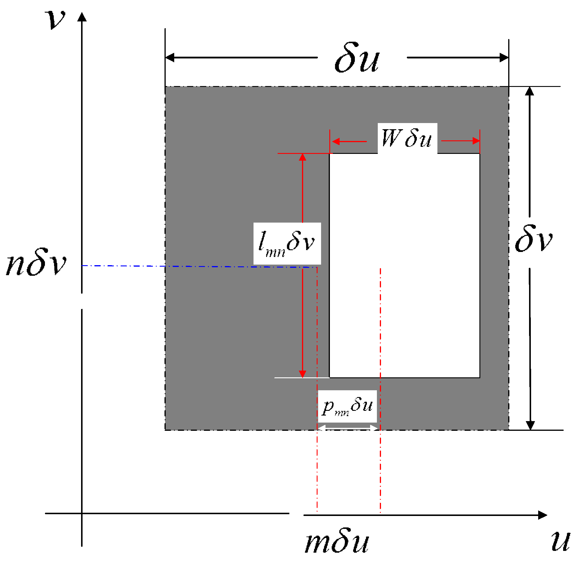
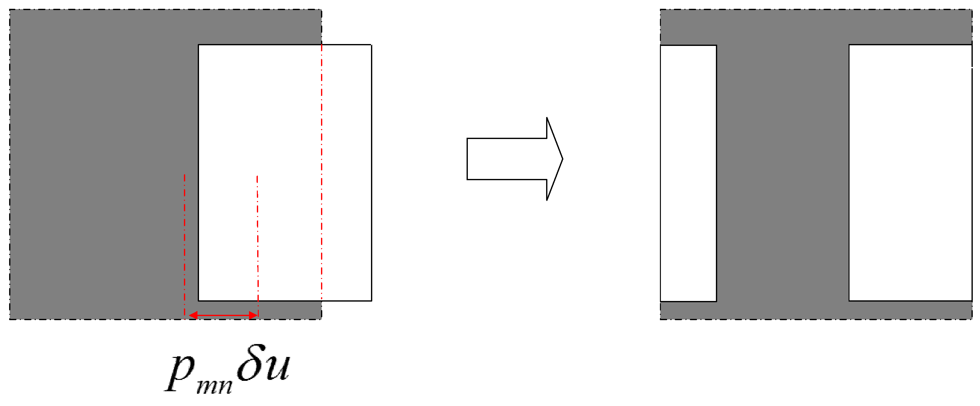
2.1. Detour Phase CGH

Assuming a plane wave is incident at an angle ${\alpha }_0$ onto a grating with a grating constant d, for the M-th order diffracted light at a diffraction angle ${\alpha }_M$, the optical path difference between adjacent rays is given by:

$$L_M=({\sin }_{{\alpha }_M}+{\sin }_{{\alpha }_0})d=M\lambda$$

(1)

When there is a misalignment p in the grating pitch of a certain part of the grating, the grating pitch changes from d to d + p. At this point, the optical path difference of the diffracted light wave becomes:

$${L_M}^{\prime }=({\sin }_{{\alpha }_M}+{\sin }_{{\alpha }_0})(d+p)$$

(2)

Therefore, in this diffraction direction, the optical path of the plane wavefront will experience the following delay:

$${\Delta }_M={L_M}^{\prime }-L_M=({\sin }_{{\alpha }_M}+{\sin }_{{\alpha }_0})p$$

(3)

The corresponding phase delay is:

$${\phi }_M={\displaystyle \frac{2\pi }{\lambda }}{\Delta }_M=2\pi Mp/d$$

(4)

The ${\phi }_M$ is referred to as the detour phase. Assume the complex amplitude distribution of the optical field on the object plane is denoted as $\tilde{U}(x,y)=a(x,y)\exp [j\varphi (x,y)]$ and its Fourier transform spectrum as $\tilde{F}(u,v)=A(u,v)\exp [j\mathsf{\Phi }(u,v)]$. To generate the CGH, sampling and quantization are performed. In the spatial domain, the sampling intervals along the x- and y-directions are $\delta x$ and $\delta y$, respectively, with a total sampling number of I × K. The complex field value at the sampling point (i, k) is $\tilde{U}(i\delta x,k\delta y)$. Similarly, in the frequency domain, the corresponding sampling intervals are $\delta u$ and $\delta v$, with a total sampling number of M × N. The spectrum value of the complex field at the sampling point (m, n) is $\tilde{F}(m\delta u,n\delta v)$. To ensure valid results, the sampling theorem must be satisfied, typically requiring I = M and K = N.

The sampled spectrum ${\tilde{F}}_{mn}=\tilde{F}(m\delta u,n\delta v)$ is also a complex number and can be expressed as ${\tilde{F}}_{mn}=C_{mn}+j{D}_{mn}$, where $C_{mn}$ and $D_{mn}$ represent the real and imaginary parts, respectively. From this, the amplitude $A_{mn}$ and phase ${\mathsf{\Phi }}_{mn}$ of the spectrum can be derived:

$$A_{mn}=\sqrt{{C_{mn}}^2+{D_{mn}}^2}$$

(5)

$${\mathsf{\Phi }}_{mn}=\arctan (D_{mn}/C_{mn})$$

(6)

Taking a binary Fourier transform hologram as an example, a sampling unit in Lohmann Type III detour-phase holography is illustrated in Figure 1. Within each sampling cell, the width W of the rectangular transmissive aperture is fixed, while the height $l_{mn}$ varies with the amplitude $A_{mn}$ at the sampling point (m, n). The distance $p_{mn}$, representing the displacement of the rectangular aperture’s center from the sampling cell’s center, is modulated by the phase ${\mathsf{\Phi }}_{mn}$ at the sampling point (m, n). In other words, the height $l_{mn}$ and position $p_{mn}$ of the rectangular aperture within each cell encode the amplitude $A_{mn}$ and phase ${\mathsf{\Phi }}_{mn}$ of the complex wavefront spectrum, respectively.

From the diffraction theory of binary Fourier holograms, the relationship between the structural parameters of rectangular apertures ($l_{mn}$, $p_{mn}$) and the amplitude $A_{mn}$ and phase ${\mathsf{\Phi }}_{mn}$ of the complex wavefront spectrum can be derived:

$$l_{mn}=k^{\prime }{A}_{mn}$$

(7)

$$p_{mn}=M^{\prime }{\mathsf{\Phi }}_{mn}/(2\pi )$$

(8)

where $k^{\prime }$ is a constant and $M^{\prime }$ is an integer, indicating that $l_{mn}$ and $p_{mn}$ are proportional to the amplitude $A_{mn}$ and phase ${\mathsf{\Phi }}_{mn}$, respectively.

Mode Overflow Correction: When ${\mathsf{\Phi }}_{mn}>\pi /2$, the rectangular aperture of the (m, n) unit overflows into the adjacent (m + 1, n) unit, and overlap occurs. The solution involves shifting the overflow portion to the opposite side of the original unit (seeing Figure 2). According to grating diffraction theory, this introduces a phase shift $2\pi$, which does not affect reconstruction [14,15,16].

2.2. Modified Off-Axis Reference Beam Cgh

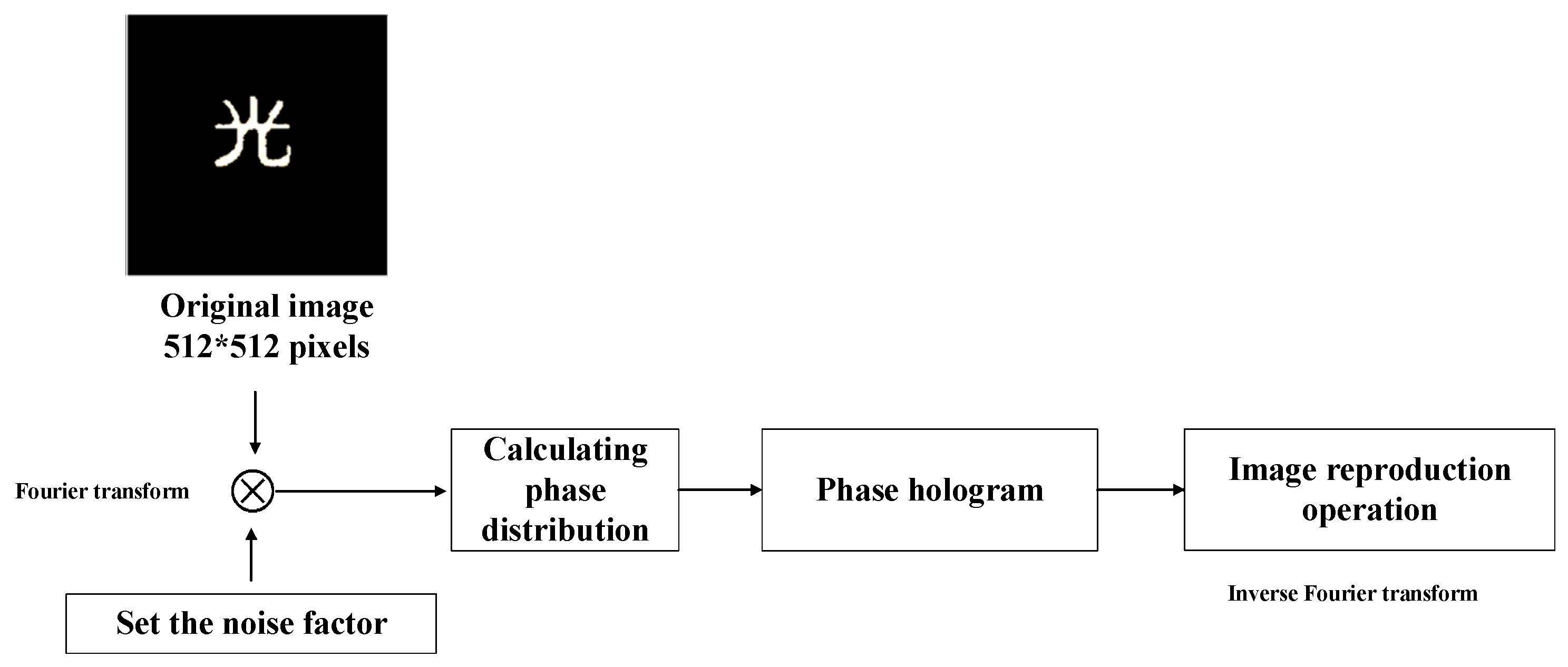
To record an object light field represented by a complex function $\tilde{U}(x,y)=A(x,y)\exp [j\phi (x,y)]$, it can be interfered with an off-axis reference light $\tilde{R}(x,y)=R\exp j\phi (2\pi \alpha x)$. The resulting off-axis hologram has a transmittance:

$$\begin{array}{l}h(x,y)={\left|\tilde{U}(x,y)+\tilde{R}(x,y)\right|}^2=\\ R^2+{\left|\tilde{A}(x,y)\right|}^2+2RA(x,y)\cos [2\pi \alpha x-\phi (x,y)]\end{array}$$

(9)

In this equation, A(x, y) and $\phi (x,y)$ represent the amplitude and phase distribution of the object optical field at position (x, y), respectively, while R and $\alpha$ denote the amplitude and carrier frequency of the reference light [17].

Burch proposed replacing $R^2+{\left|\tilde{A}(x,y)\right|}^2$ in Equation (9) with a DC bias, thereby reconstructing the transmittance function of the off-axis hologram as:

$$\begin{array}{l}h(x,y)=K+\tilde{U}(x,y)\times {\tilde{R}}^{*}(x,y)+\tilde{R}(x,y)\times {\tilde{U}}^{*}(x,y)\\ =K+2RA(x,y)\cos [2\pi \alpha x-\phi (x,y)]\end{array}$$

(10)

where K is a constant, ensuring h(x, y) is a non-negative real value for all (x, y). Normalizing ${\left|A(x,y)\right|}_{\max }=1$, taking R = 1, Equation (10) simplifies to:

$$h(x,y)=0.5\left\{1+A(x,y)\cos [2\pi \alpha x-\phi (x,y)\right\}$$

(11)

When Burch encoded and fabricated holograms using Formula (11), they directly recorded the transmittance function onto film using a microdensitometer, creating a 256-gray-level computer-generated hologram [18].

Another commonly modified off-axis hologram is the Lee Weihan-type delayed sampling hologram. This allows the complex function $\tilde{F}$ at each sampled point on the hologram to be represented by four real, non-negative values:

$$\tilde{F}=F_1+j{F}_2-F_3-j{F}_4$$

(12)

In the equation,

$$\begin{array}{c}\begin{array}{cc}{F}_1=\left\{\begin{array}{c}\left|F\right|\cos \varphi \\ 0\end{array}\right.& \begin{array}{c}\cos \varphi \ge 0\\ \cos \varphi <0\end{array}\end{array}\\ \begin{array}{cc}{F}_2=\left\{\begin{array}{c}\left|F\right|\sin \varphi \\ 0\end{array}\right.& \begin{array}{c}\cos \varphi \ge 0\\ \cos \varphi <0\end{array}\end{array}\\ \begin{array}{cc}{F}_3=\left\{\begin{array}{c}-\left|F\right|\cos \varphi \\ 0\end{array}\right.& \begin{array}{c}\cos \varphi \ge 0\\ \cos \varphi <0\end{array}\end{array}\\ \begin{array}{cc}{F}_4=\left\{\begin{array}{c}-\left|F\right|\sin \varphi \\ 0\end{array}\right.& \begin{array}{c}\cos \varphi \ge 0\\ \cos \varphi <0\end{array}\end{array}\end{array}$$

where $F_1$, $F_2$ $F_3$, and $F_4$ are all real, non-negative functions.

Essentially, this decomposes a complex vector in the complex plane by using four basis vectors: $r^{+}=(1,0)$, $r^{-}=(-1,0)$, $j^{+}=(0,1)$, and $j^{-}=(0,-1)$. Any complex vector can be expressed as:

$$\tilde{F}=F_1{r}^{+}+F_2{j}^{+}+F_3{r}^{-}+F_4{j}^{-}$$

(13)

These basis vectors have fixed angular relationships in the complex plane, with adjacent vectors separated by $\pi /2$. By applying delayed sampling technology, the original hologram plane is divided into $N\times N$ sampling points, each further subdivided into four equally spaced sub-cells. The amplitude transmittance of each sub-cell is made proportional to $F_i[mdx+(i-1)dx/4,ndy],i=1,2,3,4$. This enables the decomposition of the complex vector by using four non negative basis vectors. This method produces continuous-gray-level CGH [19].

2.3. Kinoform CGH

Assume the complex amplitude distribution of the light wave field within the kinoform CGH plane is:

$$\tilde{U}(x,y)=A\exp [j\phi (x,y)]$$

(14)

In the equation, A is assumed to be constant. A practical kinoform CHG can be generated as follows: Define the complex amplitude distribution on the kinoform CGH plane as:

$$\tilde{U}(x,y)=U_R(x,y)+j{U}_I(x,y)$$

(15)

where $U_R$ and $U_I$ are the real and imaginary parts of the light field $\tilde{U}(x,y)$, respectively.

The phase angle is calculated:

$$\phi (x,y)=\arctan [U_I(x,y)/U_R(x,y)]$$

(16)

Taking the remainder of modulus 2π from the calculated result $\phi (x,y)$, i.e., $\mathrm{mod}2\pi [\phi (x,y)]$, quantize the residual phase into M gray levels to create the kinoform CGH, which is then reduced onto film and processed via bleaching to produce the final kinoform CGH [20].

2.4. Interference-Type CGH

To capture an object light field $\tilde{U}(x,y)=A(x,y)\exp [j\phi (x,y)]$, it is typically interfered with a reference beam $\tilde{R}(x,y)=\mathrm{Re}xp(j2\pi \alpha x)$.

From Equation (9), the maximum transmittance h(x, y) of the hologram occurs when:

$$\phi (x,y)-2\pi \alpha x=2n\pi$$

(17)

and the minimum transmittance occurs when:

$$\phi (x,y)-2\pi \alpha x=2(n+1/2)\pi$$

(18)

In the equation, $n=0,\pm 1,\pm 2\dots$. Based on the formula of amplitude transmission coefficient for holograms, the computer-generated interferometric hologram function can be expressed as:

$$H(x,y)=\left\{\begin{array}{cc}1\hfill & \cos [\phi (x,y)-2\pi \alpha x]\ge \cos \pi q(x,y)\\ 0\hfill & \mathrm{Other}\mathrm{situations}\end{array}\right.$$

(19)

where $q(x,y)=\arcsin [A(x,y)]/\pi$, and the amplitude A(x, y) is normalized.

From this function, the bright fringe positions (0→1 transition points) satisfy:

$$\cos [\phi (x,y)-2\pi \alpha x]=\cos [\pi q(x,y)]$$

(20)

where $\phi (x,y)-2\pi \alpha x=2n\pi \mp \pi q(x,y)$.

In this expression, n denotes the bright fringe order, and $\alpha$ represents the carrier spatial frequency, where the negative sign corresponds to the equation of leading edges (H(x, y) transitions from 0 to 1) and the positive sign describes trailing edges (H(x, y) transitions from 1 to 0). By calculating the coordinates of bright fringes at different n values, a binary computer-generated interferometric hologram composed of width-modulated bright fringes can be effectively constructed [21].

3. Image Quality Evaluation

This study establishes a dual-metric quantitative analysis framework combining peak signal-to-noise ratio (PSNR) and the Structural Similarity Index Measure (SSIM) to assess noise in computational holographic reconstructions.

The MSE-based PSNR quantifies pixel-level signal distortion between original and reconstructed images:

$$PSNR=10*{\log }_{10}\left({\displaystyle \frac{MA{X}^2}{MSE}}\right)$$

(21)

Here, MAX denotes pixel dynamic range (255 for 8-bit images), where logarithmic conversion maps errors to decibel (dB) scale, linearly characterizing global fidelity degradation under compression or noise interference.

MSE (Mean Squared Error) formulation:

$$MSE={\displaystyle \frac{1}{MN}}{{\displaystyle \sum _{i=1}^M{\displaystyle \sum _{j=1}^N\left(I_O\left(i,j\right)-I_R\left(i,j\right)\right)}}}^2$$

(22)

where $I_O\left(i,j\right)$ and $I_R\left(i,j\right)$ represent original and reconstructed pixel values.

SSIM advances beyond pixel-wise metrics by decomposing image information into luminance (L), contrast (C), and structure (S) components, mimicking human visual system’s nonlinear perception:

$$SSIM={\displaystyle \frac{\left(2{\mu }_x{\mu }_y+C_1\right)\left(2{\sigma }_{xy}+C_2\right)}{\left({\mu }_x^2+{\mu }_y^2+C_1\right)\left({\sigma }_x^2+{\sigma }_y^2+C_2\right)}}$$

(23)

Here, ${\mu }_x$, ${\mu }_y$: local window means (luminance components); ${\sigma }_x^2$, ${\sigma }_y^2$: local window variances (contrast measures); ${\sigma }_{xy}$: cross-covariance (structural similarity). Stabilization constants C₁ and C₂ (dynamically scaled) prevent division singularity. The normalized [0, 1] SSIM range effectively evaluates texture preservation and visual naturalness in holographic reconstructions [22].

The combination of PSNR and SSIM provides a comprehensive framework for holographic noise analysis: PSNR quantifies the linear relationship between noise intensity and signal-to-noise ratio attenuation, while structural distortions induced by noise can be captured by SSIM. This combined approach ensures both mathematical rigor in noise characterization and alignment with human visual perception, thereby establishing a theoretical foundation for evaluating holographic algorithm robustness under complex noise conditions.

Figure 3 illustrates the Matlab simulation flowchart for calculating PSNR and SSIM metrics, comprising three primary steps: image preprocessing, PSNR calculation, and SSIM calculation.

4. The Verification of CGH

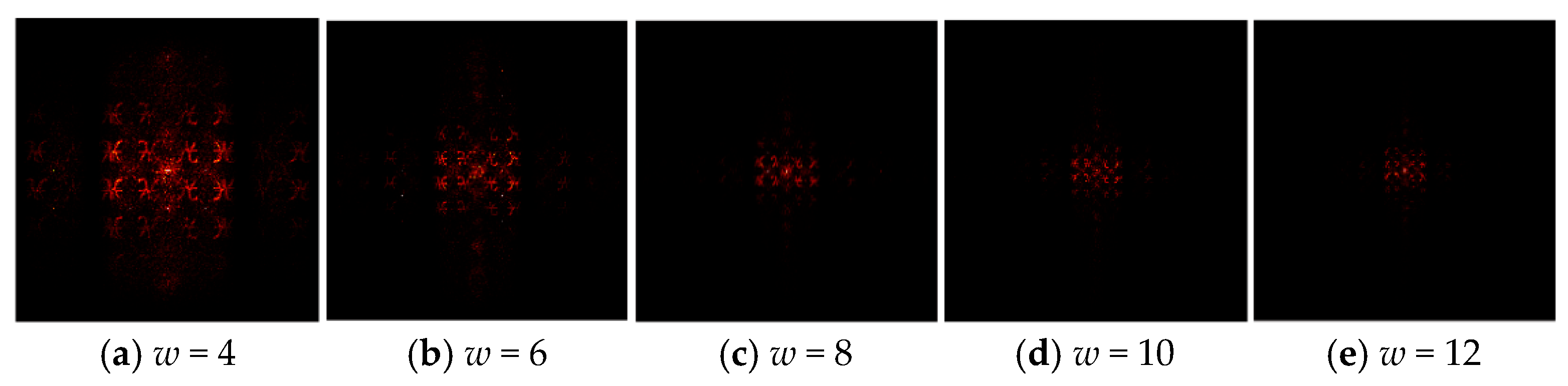
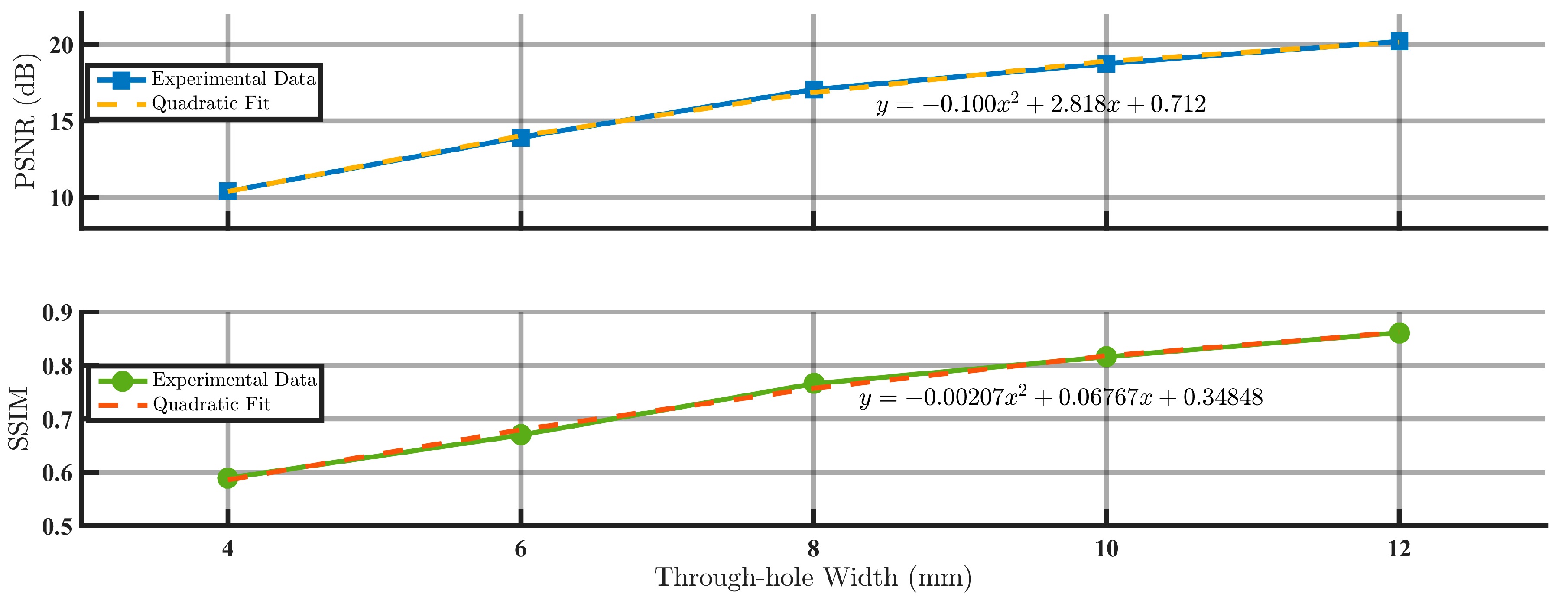
4.1. Generation of Lohmann-III Detour-Phase CGH

Figure 4 illustrates the flowchart of Lohmann Type III detour-phase CGH encoding. The object (“光” in Chinese) was initially 512 × 512 pixels but resized to 64 × 64 pixels for accelerated Matlab computation on PC platforms. Additive white Gaussian noise (AWGN) was injected with intensity controlled by the coefficient ef₁. To suppress the spectral dynamic range, tunable parameters include noise factor ef₁ and aperture width w. The object wavefield undergoes Fourier transformation followed by modulus normalization with a threshold coefficient ef₂ = 1.5. Sampling units are then embedded into the CGH via detour-phase encoding. As demonstrated in Figure 5 and Figure 6, the reconstructed images are derived from the synthesized CGH spectrum.

For computational efficiency, each CGH unit comprises s × s pixels, with aperture width w = s/2 yielding a final CGH dimension of (64 × s) × (64 × s) pixels.

(1) Assume a fixed w = 6 and ef₂ = 1.5, with ef₁ varying from 0.0 to 1.0. Figure 5 and Figure 6 show the Lohmann Type III Detour-Phase CGHs and reconstructed images under varying Gaussian noise coefficients (ef₁ = 0.0~1.0), respectively.

Calculate the PSNR and SSIM values of Lohmann Type III reconstructed images under varying Gaussian noise coefficients (ef₁ = 0.0~1.0) through the process shown in Figure 3, as shown in Figure 7.

The results (Figure 7) reveal distinct trends: PSNR monotonically decreases with the noise coefficient (18.2 dB at 0.1 to 11.59 dB at 1.0, a 36.3% reduction). A rapid decline occurs in low-noise regimes (0.1~0.3: 18.2→14.56 dB), while high-noise regimes (0.7~1.0) exhibit saturation (merely 0.71 dB reduction), indicating heightened sensitivity to low-intensity noise. SSIM shows an overall decline (0.7936→0.5925, 25.3% reduction), with minor fluctuations (0.648→0.6395) at noise coefficients 0.3~0.4, reflecting nonlinear structural degradation.

(2) Assume a fixed ef₁ = 0.8 and ef₂ = 1.5, with w adjusted from 4 to 12. The Lohmann Type III detour-phase CGHs and their reconstructed images under varying aperture widths w (w = 4~12) are presented in Figure 8 and Figure 9, respectively.

The corresponding PSNR and SSIM values for the Lohmann Type III hologram under varying aperture widths (w = 4~12) are shown in Figure 10.

Aperture width significantly impacts imaging quality (Figure 10). Increasing the aperture width from 4 to 12 enhances PSNR (10.4→20.2 dB, +94.2%) and SSIM (0.5895→0.8611, +46%), showing near-linear trends: each 2-unit aperture increase improves PSNR by ~2.45 dB and SSIM by ~0.07.

This phenomenon originates from multiple effects induced by aperture enlargement. (1) Increased photon flux effectively suppresses sensor dark current noise, thereby enhancing signal-to-noise ratio (SNR). (2) Larger apertures substantially mitigate diffraction artifacts inherent to small apertures, achieving resolution improvement from blurred states to a structural fidelity level of 0.8611. (3) Aperture expansion potentially optimizes system aberration correction capabilities.

Notably, smaller apertures (widths of 4–8) yield the most significant gains (PSNR: +64%; SSIM: +30%).

The dynamic range of the spectrum is controlled by adjusting pure-phase noise intensity (via coefficient ef₁) and aperture width w. Combined optimization of these parameters effectively balances noise suppression and imaging fidelity.

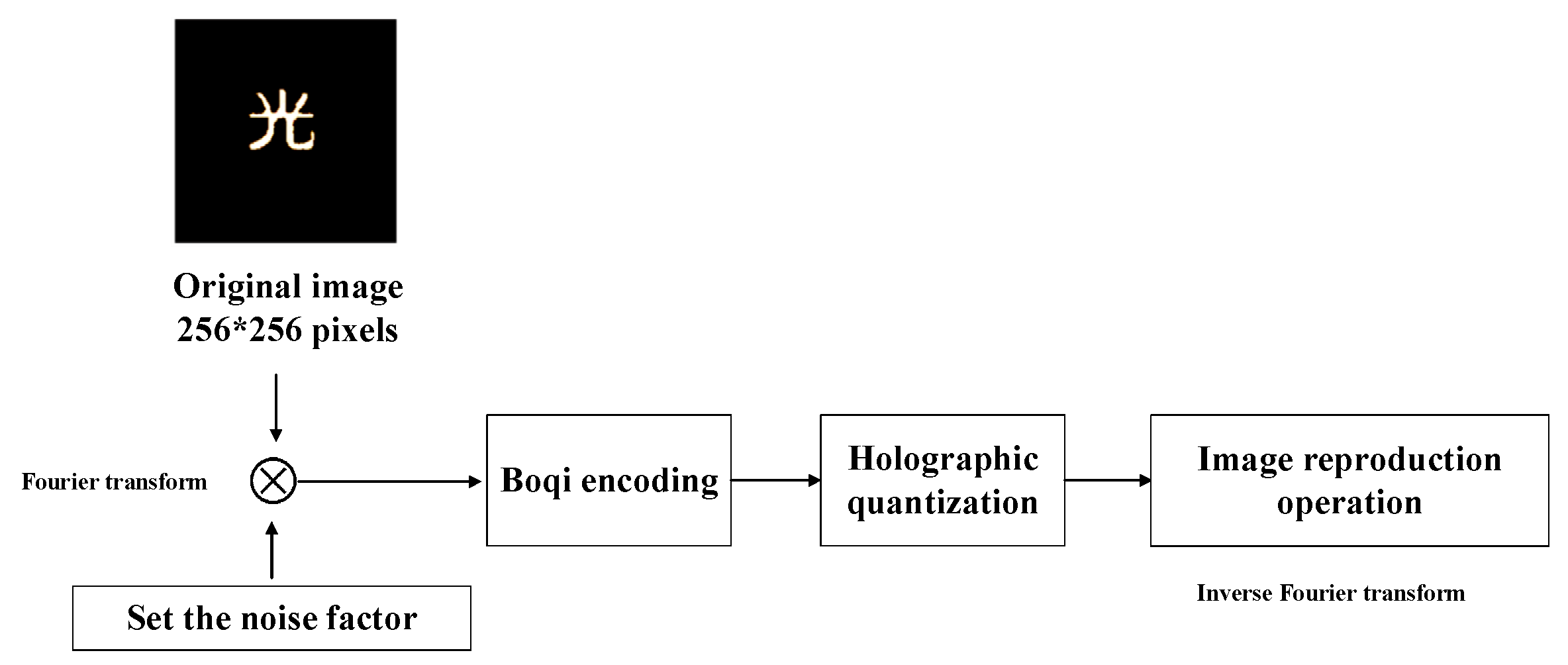
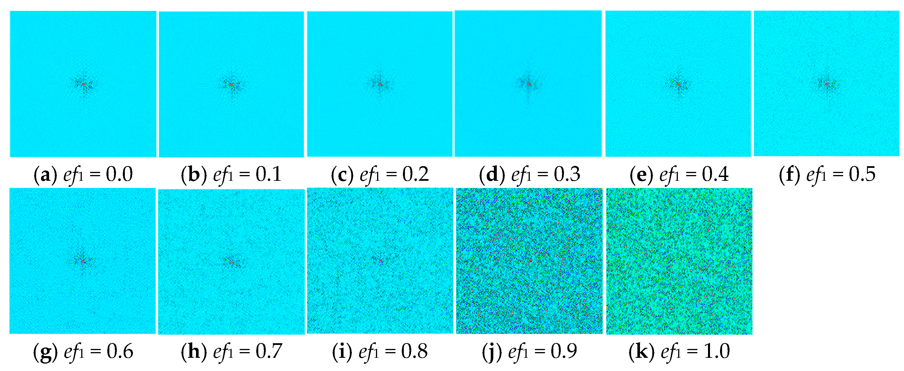
4.2. Generation of Modified Off-Axis Reference Beam CGH

This section details the simulation of Fourier-transform hologram recording and reconstruction using a modified off-axis reference beam CGH based on the Burch method. The workflow includes:

• Loading a simulated object light image (ef₁ = 0.0~1.0).
• Performing a Fast Fourier Transform (FFT) to obtain the spectrum.
• Interfering the spectrum with a tilted reference beam.
• Encoding the hologram via the Burch method to generate the CGH.
• Applying an inverse Fourier transform to the CGH to reconstruct the optical field and produce the final image.

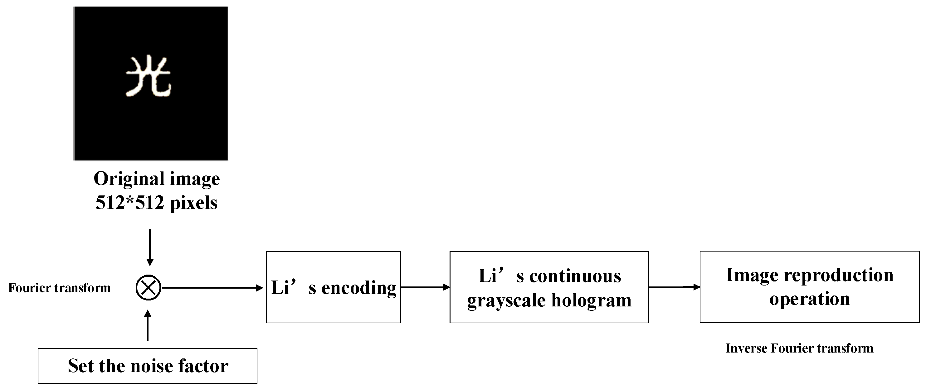
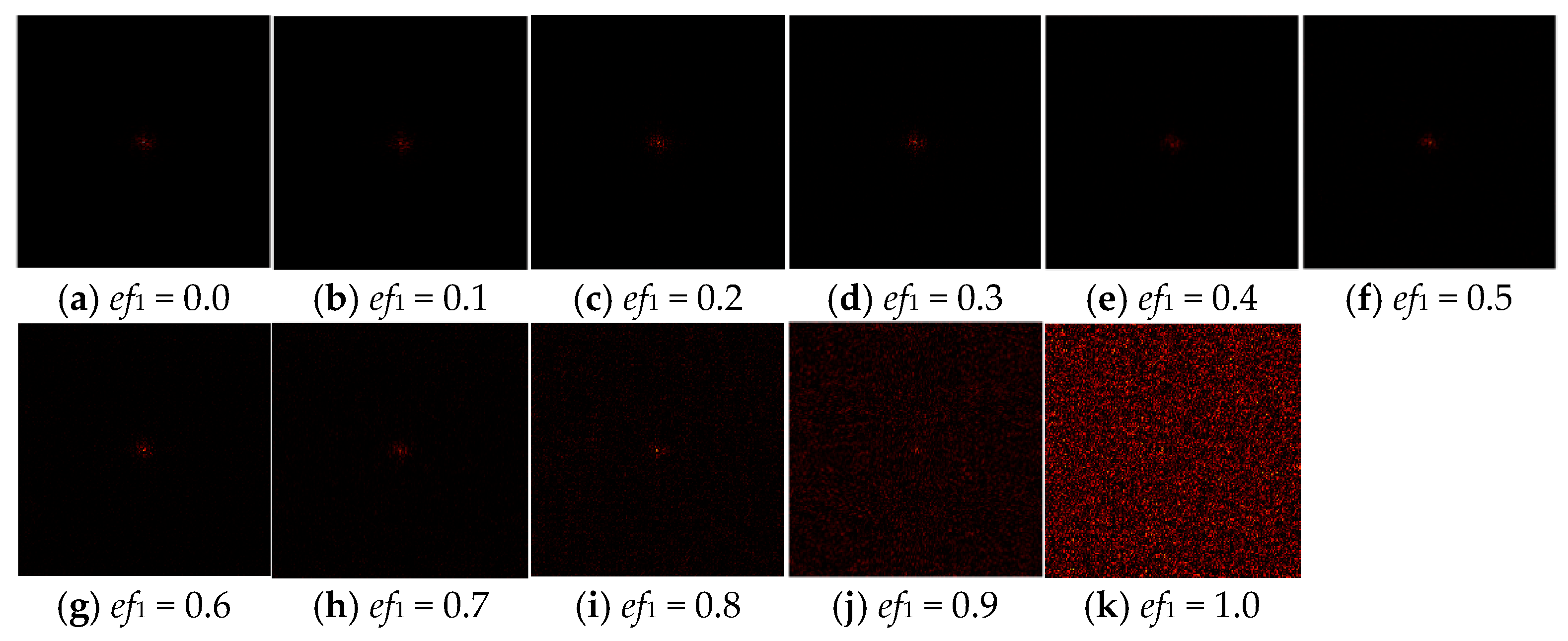
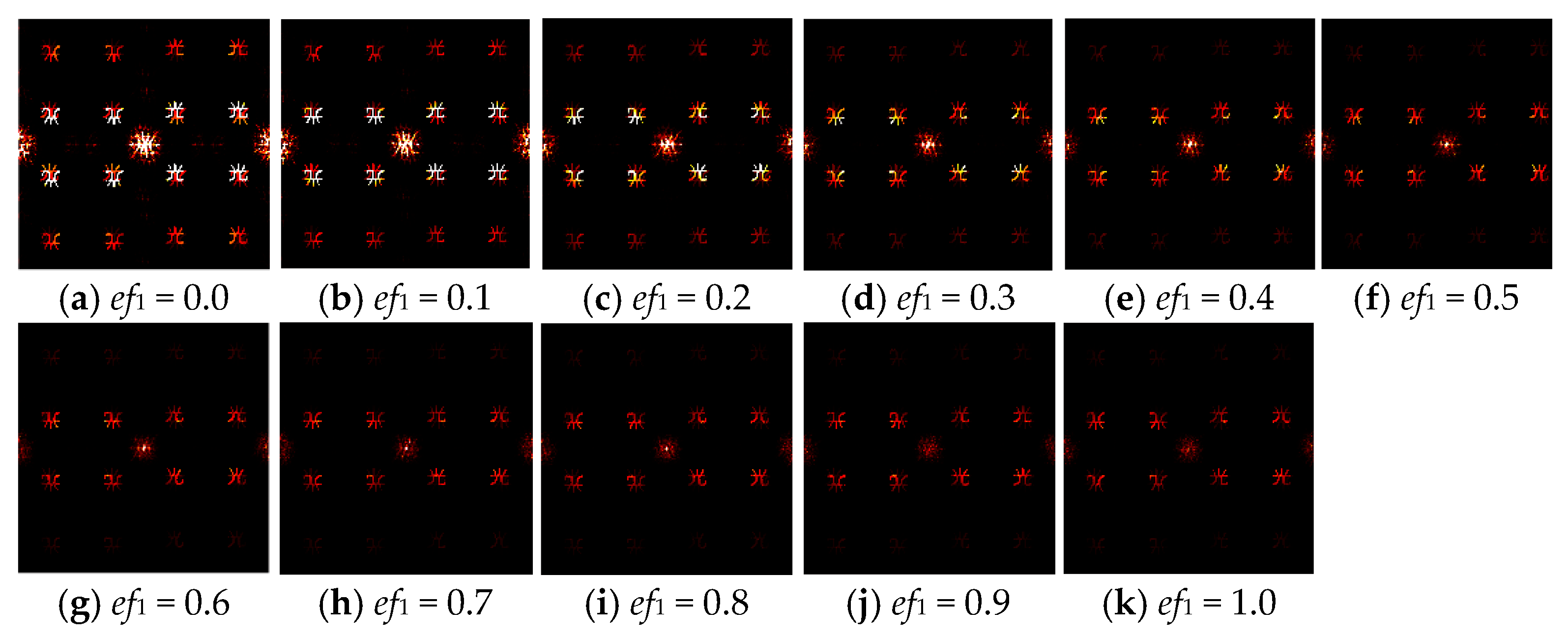
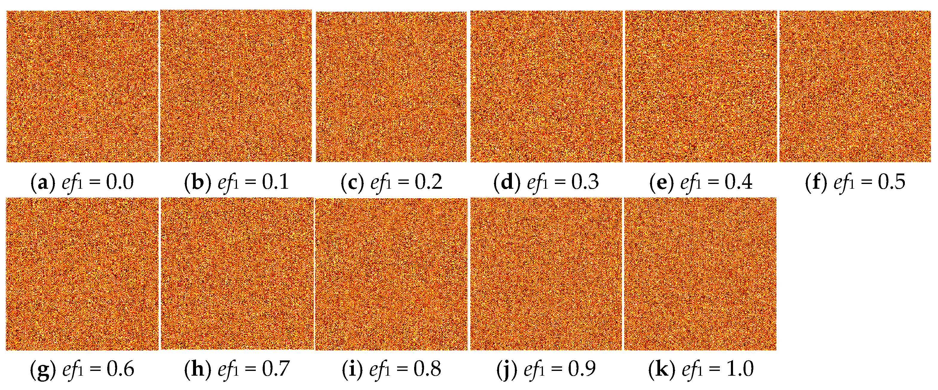
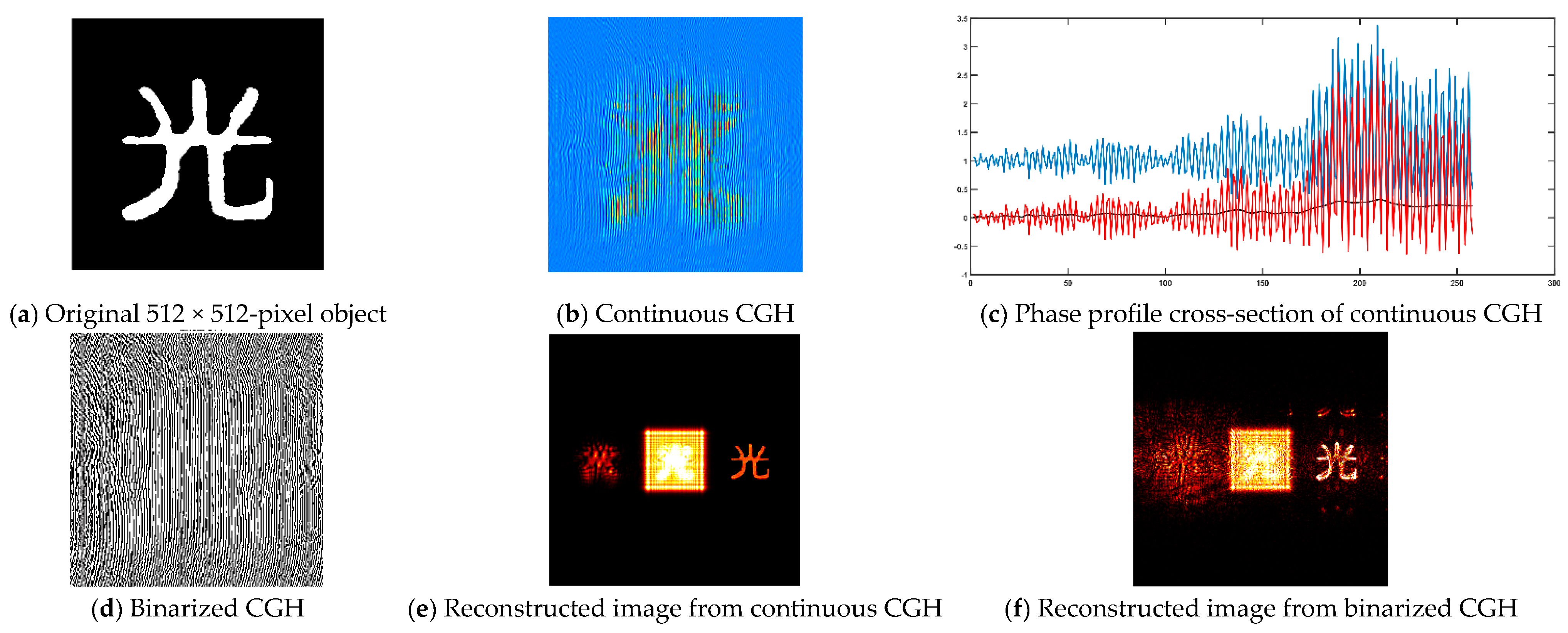
(1) Modified off-axis reference beam CGH via the Burch method

Figure 11, Figure 12 and Figure 13 illustrate the workflow of modified off-axis reference beam holography (Burch method), including the modified off-axis reference beam CGH encoding flowchart by using the Burch method (Figure 11), Burch method CGHs under varying Gaussian noise coefficients (ef₁ = 0.0~1.0) (Figure 12), and Burch method reconstructed images under varying Gaussian noise coefficients (ef₁ = 0.0 1.0) (Figure 13).

The corresponding PSNR and SSIM values of Burch-method-reconstructed images under varying Gaussian noise coefficients (ef₁ = 0.0~1.0) are shown in Figure 14.

The noise coefficient demonstrates nonlinear impacts on imaging quality (Figure 14). PSNR sharply decreases from 27.71 dB to 14.08 dB (49.2% reduction) as the noise coefficient increases from 0.1 to 1.0. SSIM shows stronger noise robustness, declining moderately from 0.9904 to 0.9042 (8.7% reduction).

Key observations: In a low-noise regime (0.1~0.5), PSNR rapidly declines by 28.3% (27.71→19.86 dB), and SSIM remains near-lossless (0.9904→0.979, 1.1% reduction). For the critical threshold (noise coefficient ≈ 0.5), PSNR falls below 20 dB (visually perceptible degradation), and SSIM retains high fidelity (0.9623). In a high-noise regime (≥0.7), there is accelerated degradation of PSNR < 16.3 dB and SSIM < 0.95; severe detail loss occurs.

Analysis reveals a signal-to-noise “saturation” effect. While high-noise PSNR reduction (29.1%) matches low-noise trends, the perceptual quality collapses abruptly. For noise-sensitive systems, maintaining a noise coefficient ≤0.3 ensures visually lossless performance (PSNR > 22.97 dB, SSIM > 0.97).

(2) Lee-encoded continuous grayscale CGHs:

In Figure 15, Figure 16 and Figure 17, the flowchart of Lee-encoded continuous grayscale CGH encoding, Lee-encoded continuous grayscale CGHs under varying Gaussian noise coefficients (ef₁ = 0.0~1.0), and Lee-encoded continuous grayscale reconstructed images under varying Gaussian noise coefficients (ef₁ = 0.0~1.0) are displayed. Lee’s method decomposes complex functions into four orthogonal non-negative components (Equations (12) and (13)). By applying delayed sampling, each sampling unit is divided into four subgrids corresponding to distinct basis vectors. Noise is distributed across multiple components during decomposition, with partial energy canceled via orthogonality, thereby reducing noise sensitivity in individual components. Grayscale encoding records component amplitudes through multi-level transmittance, smoothing noise-induced fluctuations and avoiding abrupt distortions inherent to binary encoding.

PSNR and SSIM values of Lee-encoded continuous grayscale reconstructed images under varying Gaussian noise coefficients (ef₁ = 0.0~1.0) are shown in Figure 18.

Results (Figure 18) demonstrate stage-specific noise impacts on image quality metrics. PSNR decreases rapidly by 29% (27.88 dB→19.79 dB) at noise coefficients 0.1~0.5, followed by marginal attenuation (0.7 dB, 19.79→19.09 dB) in the high-noise regime (0.5~1.0), confirming its “saturation attenuation” approaching the theoretical noise-dominant limit. In contrast, SSIM exhibits a 3.9% reduction (0.9749→0.9365) at 0.1~0.3 noise and merely a 1.5% decline (0.9365→0.9216) at 0.3~1.0, sustaining structural fidelity >0.92 throughout, which verifies its exceptional robustness under intense noise.

A mechanistic analysis reveals that the accelerated PSNR decay originates from linear noise energy accumulation directly degrading SNR, whereas SSIM stability arises from effective preservation of macroscopic structural features (edges, textures) and contrast characteristics under noise interference.

(3) Lee-encoded binary CGHs

In Figure 19, Figure 20 and Figure 21, the flowchart of Lee-encoded binary CGH encoding, Lee-encoded binary CGHs under varying Gaussian noise coefficients (ef₁ = 0.0~1.0), and Lee-encoded binary reconstructed images under varying Gaussian noise coefficients (ef₁ = 0.0~1.0) are displayed. Pure phase noise (ef₁) randomizes the phase of the object wavefront’s complex amplitude, inducing amplitude distribution shifts in the four decomposed basis components and localized adjustments to subgrid apertures.

PSNR and SSIM values of Lee-encoded binary reconstructed images under varying Gaussian noise coefficients (ef₁ = 0.0~1.0) are shown in Figure 22.

Experimental results (Figure 22) reveal that PSNR exhibits continuous attenuation, declining by 29% (22.34 dB→15.83 dB) as noise increases from 0.1 to 1.0, with a sharper reduction of 16.8% (22.34→18.61 dB) in low-noise regimes (0.1~0.4) versus 13.6% (18.32→15.83 dB) at higher noise levels (0.5~1.0), indicating SNR saturation under noise dominance. In contrast, SSIM shows only a 3.9% overall decline (0.9294→0.893), with an anomalous 0.2% increase (0.9131→0.9153) at 0.4~0.5 noise. As a result of noise–content interactions, low-contrast distortion masking at specific noise levels and edge-sharpening effects induced by high-frequency noise may temporarily enhancing structural similarity.

These findings demonstrate SSIM’s superior robustness to noise interference compared to PSNR. At noise coefficients of ef₁ ≥ 0.5, PSNR enters a slow-decay noise-dominant state, while SSIM maintains its structural fidelity above 0.89, underscoring its evaluative advantage in noisy scenarios.

4.3. Kinoform CGHs

Figure 23, Figure 24 and Figure 25 illustrate the flowchart of Kinoform CGH encoding, Kinoform CGHs under varying Gaussian noise coefficients (ef₁ = 0.0~1.0), and Kinoform reconstructed images under varying Gaussian noise coefficients (ef₁ = 0.0~1.0). Kinoforms CGHs encode information as relief-phase profiles on recording elements.

PSNR and SSIM values of Kinoform reconstructed images under varying Gaussian noise coefficients (ef₁ = 0.0~1.0) are shown in Figure 26.

As shown in Figure 26, noise coefficients exhibit distinct impacts on image quality metrics. PSNR declines continuously from 16.59 dB to 12.43 dB (25% reduction) as noise increases from 0.1 to 1.0, with the steepest drop (10.2%) occurring at low noise (0.1~0.3), consistent with the inverse-square relationship between noise energy and SNR. At higher noise levels (0.5~1.0), the reduction narrows to 10.9% (13.95→12.43 dB), indicating SNR saturation approaching noise dominance. In contrast, SSIM shows only a 4.0% decline (0.7551→0.7248) across the noise range, with <1.0% reduction for coefficients ≥ 0.5, highlighting its strong noise robustness.

Mechanistic analysis reveals that PSNR sensitivity stems from its direct response to global energy variations, while SSIM stability benefits from preserved macroscopic structural features (edges, textures) under high noise. This discrepancy may be attributed to the experimental image characteristics (low texture, high contrast) and noise properties (uniform Gaussian distribution).

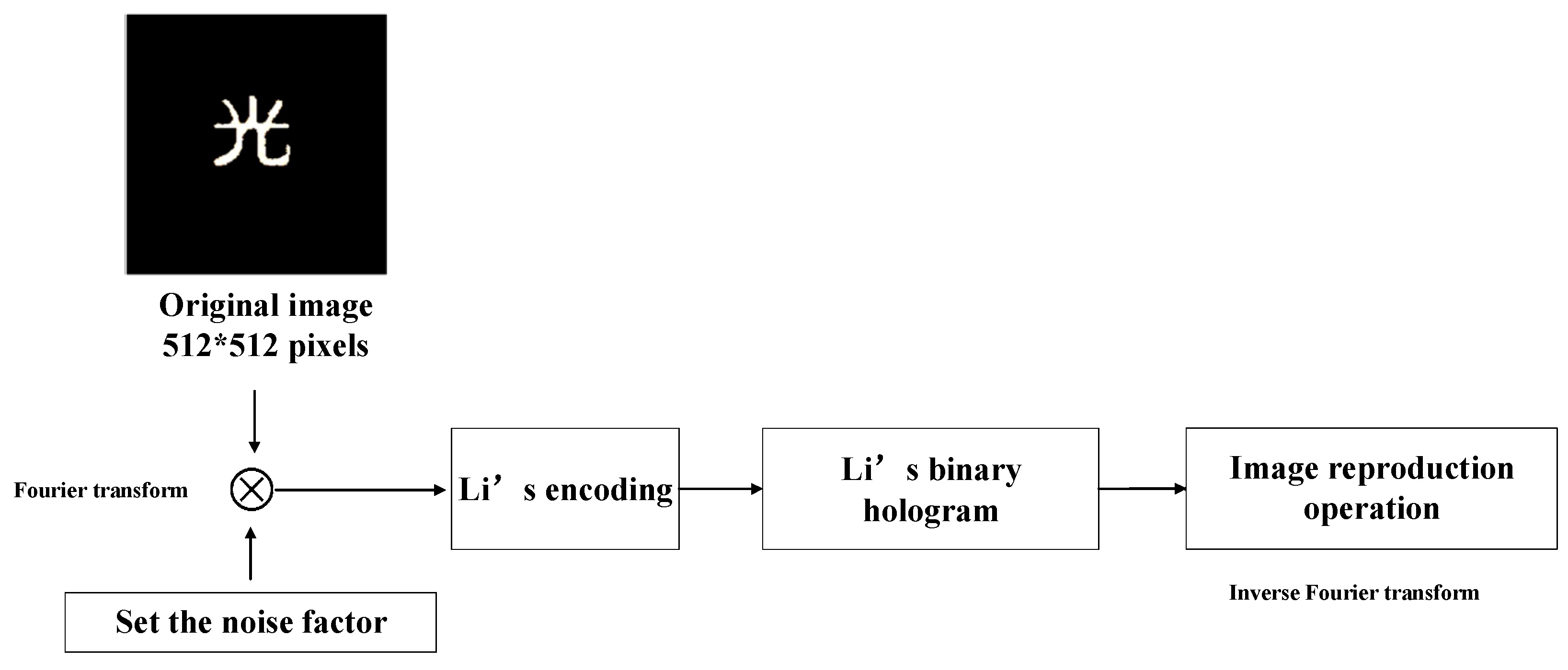
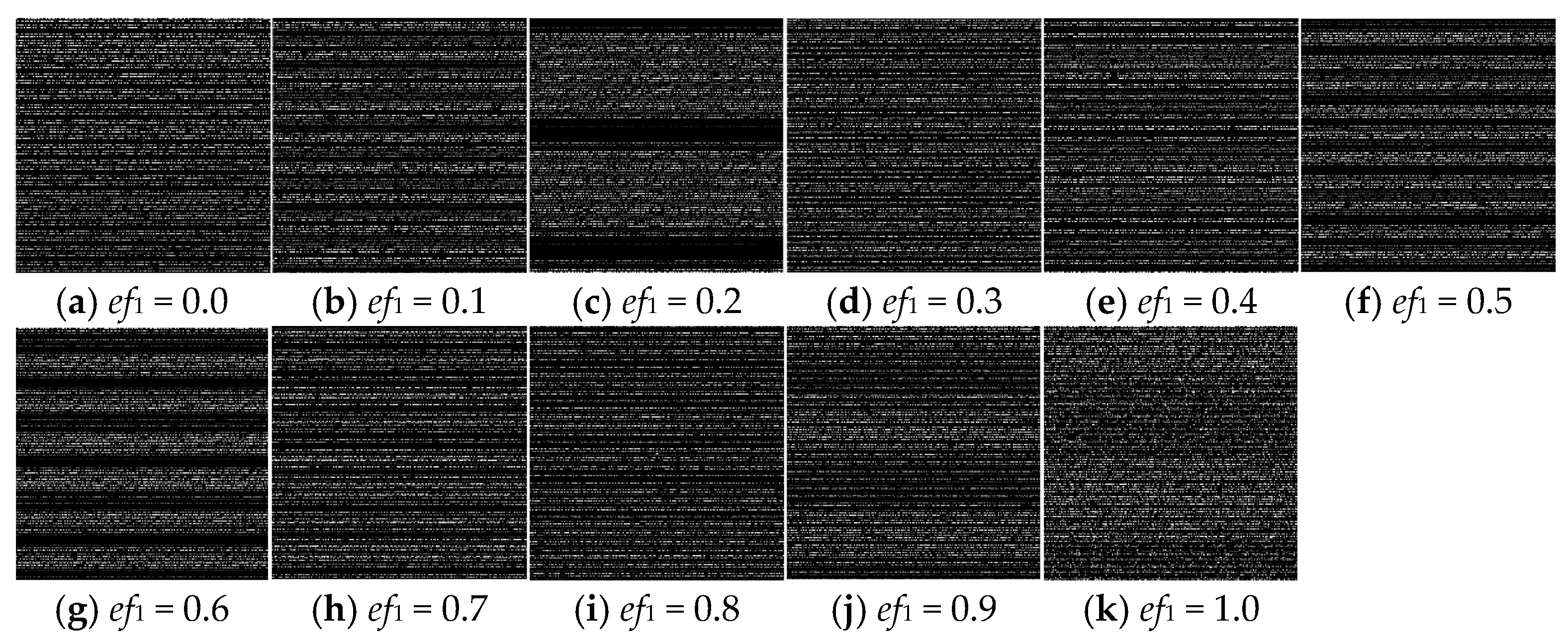
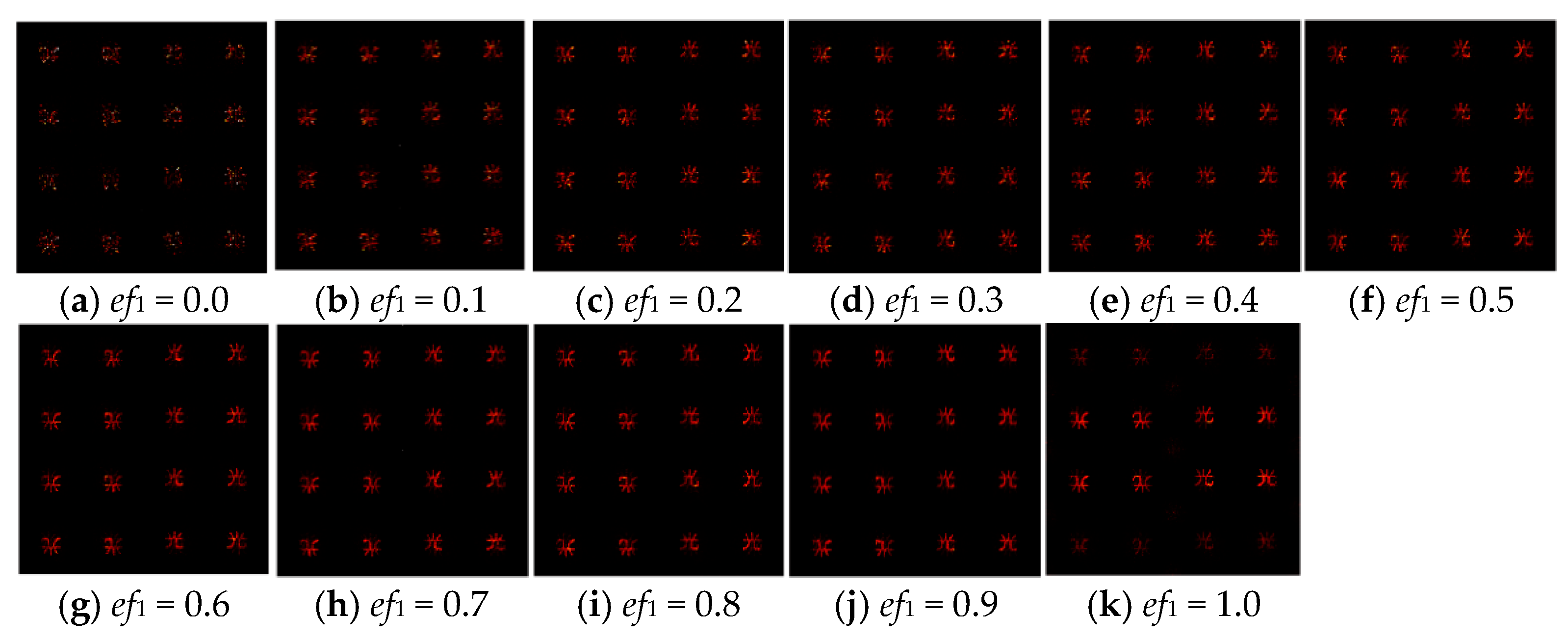
4.4. Interference Type CGHs

While previous simulations focused on Fourier transform holography, computational holography extends beyond this approach. We conducted experiments using Fresnel holography with a He-Ne laser (λ = 632.8 nm). The flowchart included computation of the diffracted object field, generation of continuous CGHs via object–reference beam interference, binarization of interference patterns to produce binary CGHs, and reconstruction of binary CGHs under illumination.

The continuous CGH (Figure 27b,e) exhibits intact interference fringes and high reconstruction fidelity, preserving both amplitude and phase information of the original wavefield. In contrast, the binarized CGH (Figure 27d,f) discretizes fringe transmittance into 0/1 levels, introducing quantization artifacts (edge blurring and texture distortion) that significantly degrade reconstruction quality.

Fundamentally, continuous CGH encodes amplitude through fringe contrast (brightness modulation), while binarization enforces amplitude quantization via thresholding, resulting in dynamic range compression and high-frequency detail loss.

5. Conclusions

This study systematically evaluates the noise robustness and imaging performance of four computational holography encoding algorithms (detour-phase, modified off-axis reference, kinoform, and interference holography) through a dual-metric framework combining PSNR and SSIM. Key findings include:

(1)

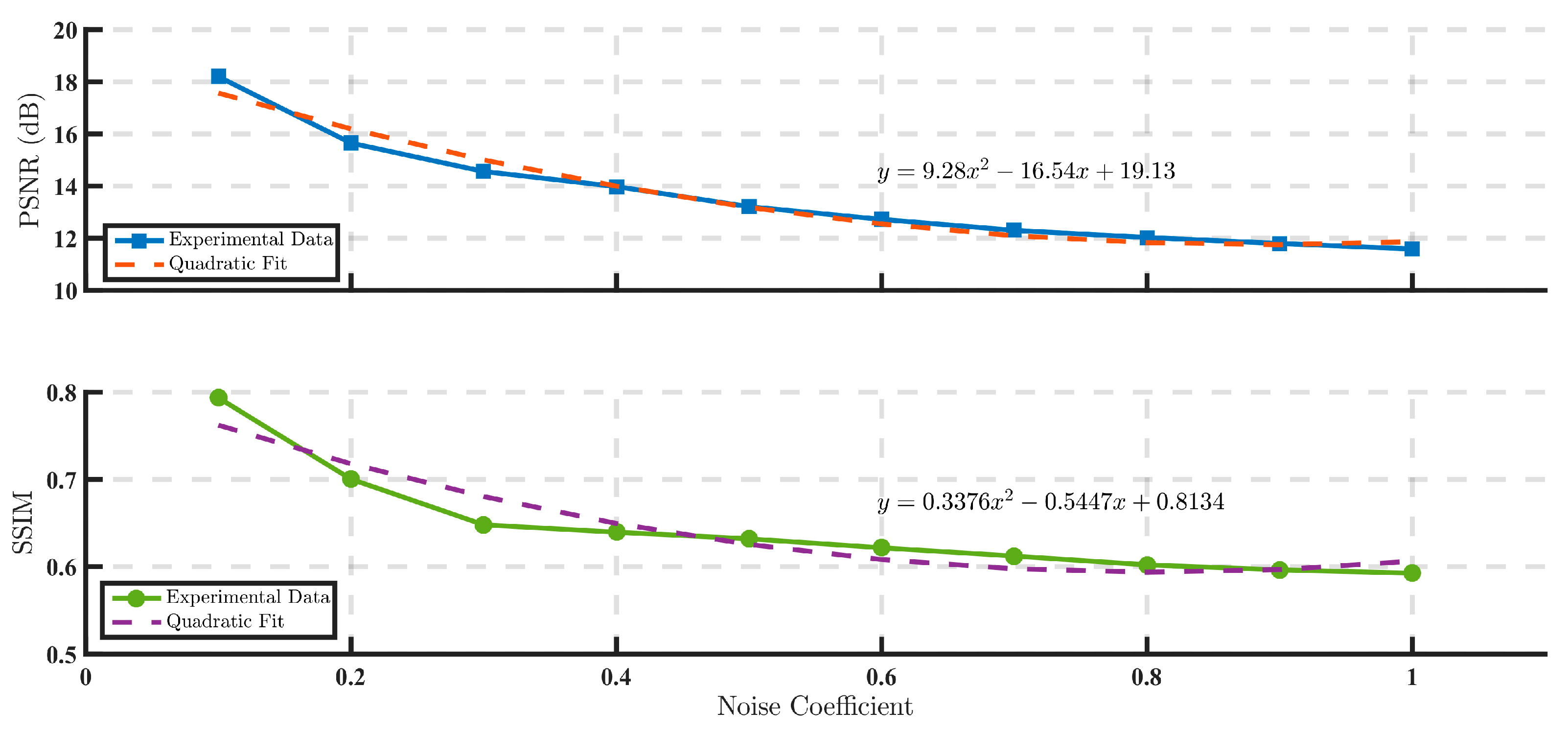
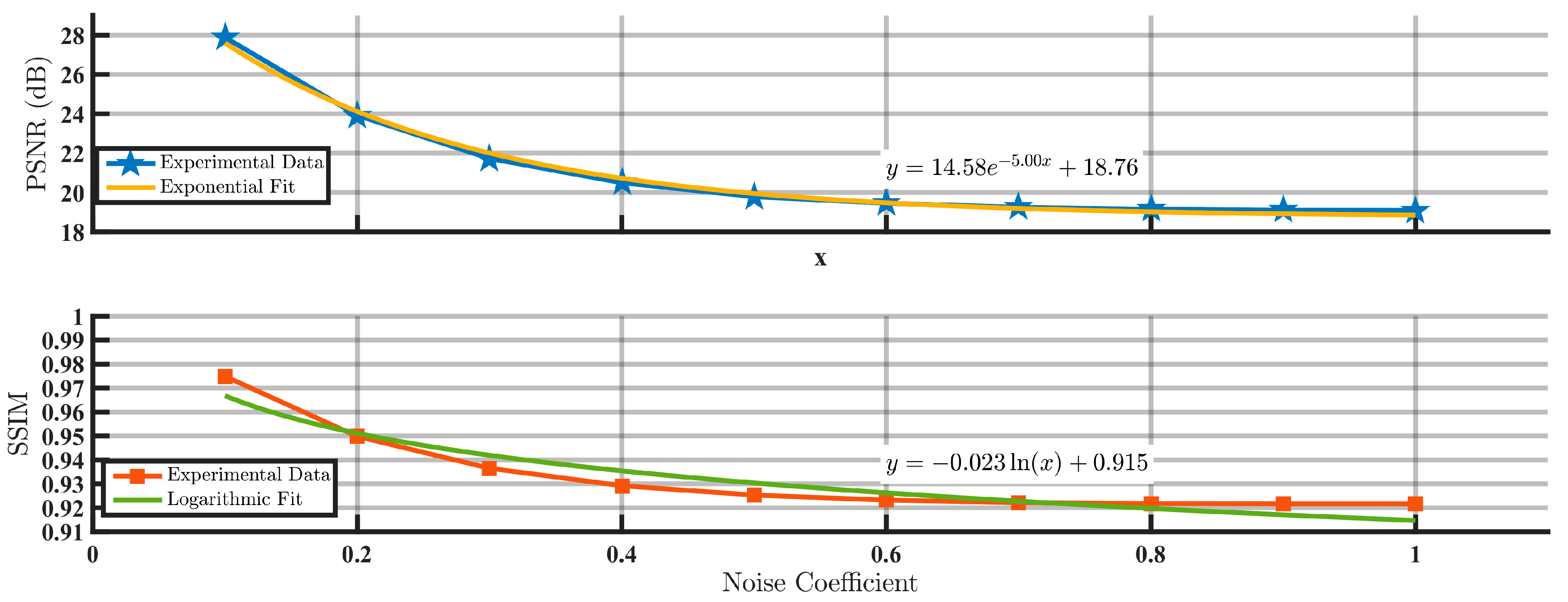
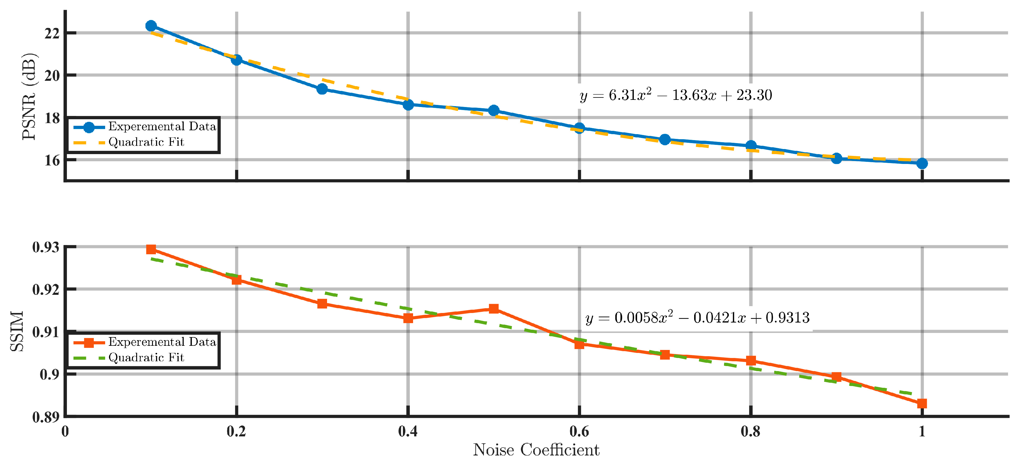
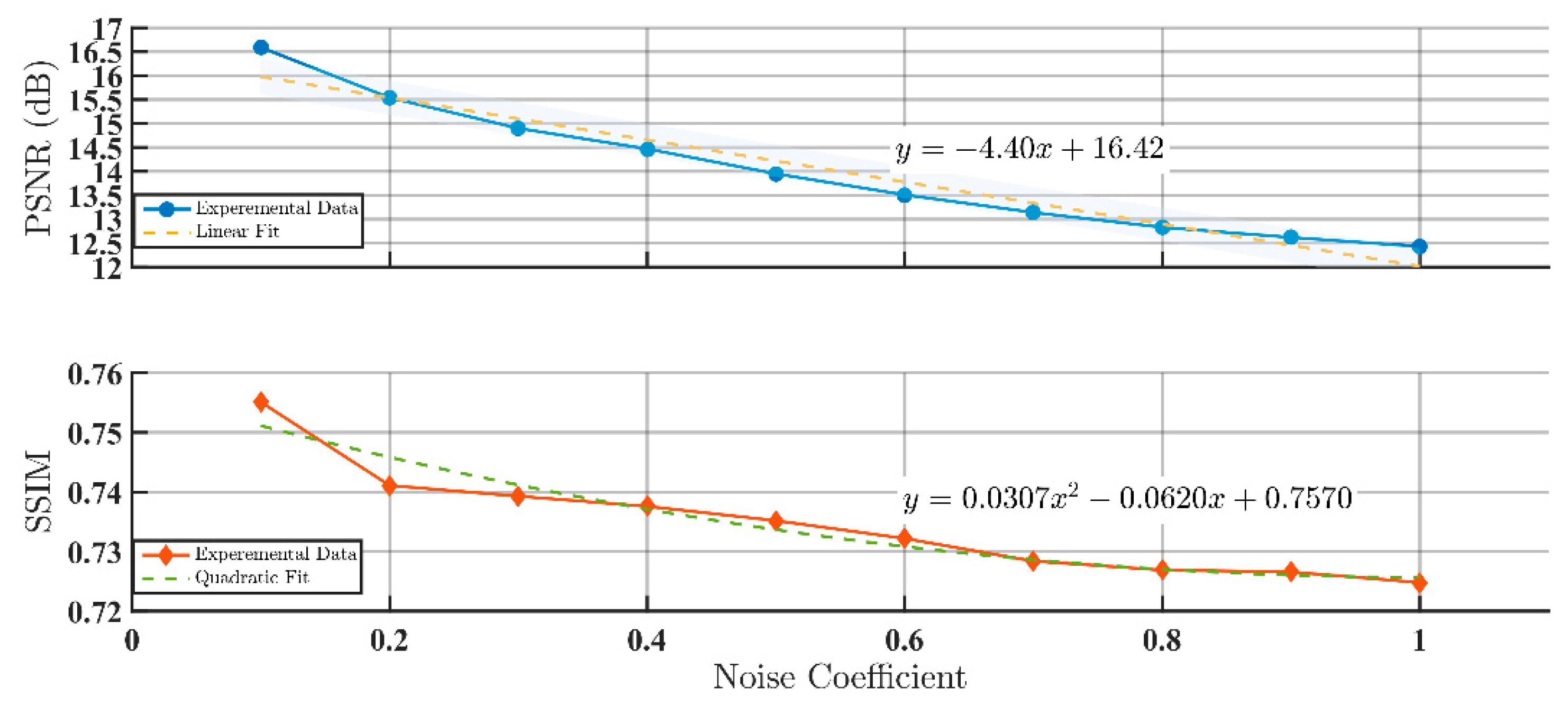
Noise–SNR Correlation: PSNR exhibits monotonic decay with increasing noise coefficients, showing accelerated reduction in low-noise regimes (≤0.3, e.g., 36.3% drop for Lohmann III) and saturation attenuation in high-noise regimes (≥0.5, e.g., 10.9% reduction for kinoforms), confirming PSNR’s sensitivity to low noise but limited capacity in noise-dominant scenarios.

(2)

SSIM Robustness: SSIM demonstrates superior stability across all encoding methods, maintaining 0.9042 for modified Burckhardt encoding at noise coefficient 1.0 and sustaining SSIM >0.92 throughout Lee’s grayscale encoding, validating its effectiveness in preserving edge/texture features to suppress visual distortions.

(3)

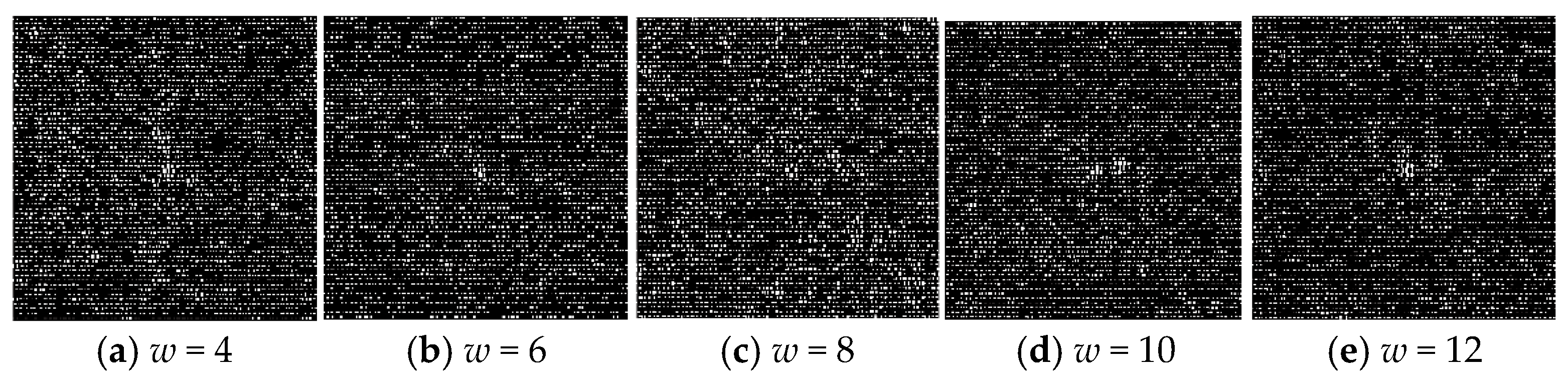
Encoding Optimization: Noise resistance improves significantly through method refinement. Lee’s grayscale encoding achieves 19.09 dB PSNR at noise coefficient 1.0 (21% improvement over binary encoding), while Lohmann III enhances PSNR/SSIM by 94.2%/46% via aperture expansion (4→12), with most pronounced gains at low apertures (4→8).

(4)

Interference Holography: Continuous CGHs outperform binarized versions in reconstruction clarity (Figure 27e vs. Figure 27f), as amplitude information preservation in interference fringes mitigates grayscale dynamic range compression-induced distortion.

(5)

Noise Thresholds: Visual lossless quality (SSIM > 0.95) is achievable at noise coefficients ≤0.3, while imaging usability at ≥0.7 requires combined strategies like noise-resistant encoding (e.g., Li’s grayscale) or aperture optimization.

These conclusions provide theoretical foundations for optimizing encoding strategies and parameters in computational holography systems operating under high-noise conditions.

References

1. Wei, C.; Zhou, R.; Ma, H.; Pi, D.; Wei, J.; Wang, Y.; Liu, J. Holographic display using layered computer-generated volume hologram. Opt. Express 2023, 31, 25153–25164. [Google Scholar] [CrossRef] [PubMed]
2. Ding, X.; Chang, C.; Dai, B.; Wang, Q.; Zhang, D.; Zhuang, S. Real-time holographic 3D display using Split-Lohmann Fresnel computer-generated hologram. Opt. Express 2024, 32, 40175–40189. [Google Scholar] [CrossRef] [PubMed]
3. Gan, Z.; Peng, X.; Hong, H. An Evaluation Model for Analyzing the Overlay Error of Computer-generated Holograms. Curr. Opt. Photonics 2020, 4, 277–285. [Google Scholar]
4. Shi, L.; Li, B.; Matusik, W. End-to-end learning of 3D phase-only holograms for holographic display. Light Sci. Appl. 2022, 11, 2176–2193. [Google Scholar] [CrossRef]
5. Zhao, T.; Liu, J.; Gao, Q.; He, P.; Han, Y.; Wang, Y. Accelerating computation of CGH using symmetric compressed look-up-table in color holographic display. Opt. Express 2018, 26, 16063–16073. [Google Scholar] [CrossRef]
6. Gao, C.; Liu, J.; Li, X.; Xue, G.; Jia, J.; Wang, Y. Accurate compressed look up table method for CGH in 3D holographic display. Opt. Express 2015, 23, 33194–33204. [Google Scholar] [CrossRef]
7. Noghani, F.E.; Tofighi, S.; Bahrampour, A.R. The theoretical investigation of the proposed optical fiber torsion sensor based on computer-generated-hologram (CGH). Opt. Commun. 2020, 463, 125323. [Google Scholar] [CrossRef]
8. Xiao, X.; Yu, Q.; Zhu, Z. Encoding method of CGH for highly accurate optical measurement based on non-maxima suppression. Chin. Opt. Lett. 2017, 15, 45–49. [Google Scholar]
9. Zhou, J.; Jiang, L.; Yu, G.; Wang, J.; Wu, Y.; Wang, J. Solution to the issue of high-order diffraction images for cylindrical computer-generated holograms. Opt. Express 2024, 32, 14978–14993. [Google Scholar] [CrossRef]
10. Yao, Y.; Zhang, Y.; Fu, Q.; Duan, J.; Zhang, B.; Cao, L.; Poon, T.C. Adaptive layer-based computer-generated holograms. Opt. Lett. 2024, 49, 1481–1484. [Google Scholar] [CrossRef]
11. Nanmaran, R.; Luminasree, B. Development of Wavelet Transform-Based Image Fusion Technique with Improved PSNR for CT and PET Images in Comparison with Discrete Cosine Transform-Based Image Fusion Technique. ECS Trans. 2022, 107, 13185. [Google Scholar]
12. Francesco, M.; Gabriele, S. Convergence results in image interpolation with the continuous SSIM. SIAM J. Imaging Sci. 2022, 15, 1977–1999. [Google Scholar]
13. Martini, M.G. Measuring Objective Image and Video Quality: On the Relationship Between SSIM and PSNR for DCT-Based Compressed Images. IEEE Trans. Instrum. Meas. 2025, 74, 5007813. [Google Scholar] [CrossRef]
14. Zhu, B.; Liu, H.; Liu, Y.; Yan, X.; Chen, Y.; Chen, X. Second-harmonic computer-generated holographic imaging through monolithic lithium niobate crystal by femtosecond laser micromachining. Opt. Lett. 2020, 45, 4132–4135. [Google Scholar] [CrossRef]
15. Călin, B.Ş.; Preda, L.; Jipa, F.; Zamfirescu, M. Laser fabrication of diffractive optical elements based on detour-phase computer-generated holograms for two-dimensional Airy beams. Appl. Opt. 2018, 57, 1367–1372. [Google Scholar] [CrossRef]
16. Wu, H.Y.; Chavel, P.; Joyeux, D.; Brunol, J. Fresnel detour-phase circular computer generated holograms. Opt. Commun. 1983, 45, 155–159. [Google Scholar] [CrossRef]
17. Liu, Z.; Xie, Y.; Zhu, W.; Fu, Q.; Gao, F.; Li, G.; Wang, Y.; Su, X.; Zhang, B.; Kumar, S. Flexible Method for Generating Arbitrary Vector Beams Based on Modified Off-Axis Interference-Type Hologram Encoding. Photonics 2022, 9, 949. [Google Scholar] [CrossRef]
18. Sun, P.; Wei, Y.; Wang, Z.; Luo, Y. An analysis of the influence of the color rendition of images reconstructed from full-color computer-generated Fourier-transform holograms. Phys. Scr. 2014, 89, 035502. [Google Scholar] [CrossRef]
19. Burckhardt, C.B. A Simplification of Lee’s Method of Generating Holograms by Computer. Appl. Opt. 1970, 9, 1949. [Google Scholar] [CrossRef]
20. Cruz-López, M.-L.; González-Velázquez, K.G. Analysis of random-phase distributions and Perlin noise in CGH: A study of its effects on Fourier and Fresnel holograms reconstruction. Opt. Eng. 2020, 59, 102419. [Google Scholar]
21. Athira, T.S.; Yadu Krishnan, K.T.; Naik, D.N. Nonlinear detection of phase difference in optical interference using computer generated hologram assisted common-path three-beam interferometry. Indian J. Phys. 2024. [Google Scholar] [CrossRef]
22. Setiadi, D.R.I.M. PSNR vs SSIM: Imperceptibility quality assessment for image steganography. Multimed. Tools Appl. 2021, 80, 8423–8444. [Google Scholar] [CrossRef]
Figure 1. Schematic of a sampling unit in Lohmann Type III detour-phase holography.
Applsci 15 06047 g001
Figure 2. Mode overflow correction algorithm for Lohmann Type III holograms.
Applsci 15 06047 g002
Figure 3. Matlab simulation flowchart for calculating PSNR and SSIM metrics.
Applsci 15 06047 g003
Figure 4. The flowchart of Lohmann Type III detour-phase CGH encoding.
Applsci 15 06047 g004
Figure 5. Lohmann Type III detour-phase CGHs under varying Gaussian noise coefficients (ef1 = 0.0~1.0).
Applsci 15 06047 g005
Figure 6. Lohmann Type III detour-phase reconstructed images under varying Gaussian noise coefficients (ef1 = 0.0~1.0).
Applsci 15 06047 g006
Figure 7. PSNR and SSIM values of Lohmann Type III reconstructed images under varying Gaussian noise coefficients (ef1 = 0.0~1.0).
Applsci 15 06047 g007
Figure 8. Lohmann Type III detour-phase CGHs under varying aperture widths w (w = 4~12).
Applsci 15 06047 g008
Figure 9. Lohmann Type III detour-phase reconstructed images under varying aperture widths w (w = 4~12).
Applsci 15 06047 g009
Figure 10. PSNR and SSIM values for Lohmann Type III hologram under varying aperture widths (w = 4~12).
Applsci 15 06047 g010
Figure 11. The modified off-axis reference beam CGH encoding flowchart by using the Burch method.
Applsci 15 06047 g011
Figure 12. Burch method CGHs under varying Gaussian noise coefficients (ef1 = 0.0~1.0).
Applsci 15 06047 g012
Figure 13. Burch method reconstructed images under varying Gaussian noise coefficients (ef1 = 0.0~1.0).
Applsci 15 06047 g013
Figure 14. PSNR and SSIM values of Burch-method-reconstructed images under varying Gaussian noise coefficients (ef1 = 0.0~1.0).
Applsci 15 06047 g014
Figure 15. The flowchart of Lee-encoded continuous grayscale CGH encoding.
Applsci 15 06047 g015
Figure 16. Lee-encoded continuous grayscale CGHs under varying Gaussian noise coefficients (ef1 = 0.0~1.0).
Applsci 15 06047 g016
Figure 17. Lee-encoded continuous grayscale reconstructed images under varying Gaussian noise coefficients (ef1 = 0.0~1.0).
Applsci 15 06047 g017
Figure 18. PSNR and SSIM values of Lee-encoded continuous grayscale reconstructed images under varying Gaussian noise coefficients (ef1 = 0.0~1.0).
Applsci 15 06047 g018
Figure 19. The flowchart of Lee-encoded binary CGH encoding.
Applsci 15 06047 g019
Figure 20. Lee-encoded binary CGHs under varying Gaussian noise coefficients (ef1 = 0.0~1.0).
Applsci 15 06047 g020
Figure 21. Lee-encoded binary reconstructed images under varying Gaussian noise coefficients (ef1 = 0.0~1.0).
Applsci 15 06047 g021
Figure 22. PSNR and SSIM values of Lee-encoded binary reconstructed images under varying Gaussian noise coefficients (ef1 = 0.0~1.0).
Applsci 15 06047 g022
Figure 23. The flowchart of Kinoform CGH encoding.
Applsci 15 06047 g023
Figure 24. Kinoform CGHs under varying Gaussian noise coefficients (ef1 = 0.0~1.0) (Part).
Applsci 15 06047 g024
Figure 25. Kinoform reconstructed images under varying Gaussian noise coefficients (ef1 = 0.0~1.0).
Applsci 15 06047 g025
Figure 26. PSNR and SSIM values of Kinoform reconstructed images under varying Gaussian noise coefficients (ef1 = 0.0~1.0).
Applsci 15 06047 g026
Figure 27. The synthesis and reconstruction of computer-generated interferometric hologram in Fresnel domain.
Applsci 15 06047 g027
Disclaimer/Publisher’s Note: The statements, opinions and data contained in all publications are solely those of the individual author(s) and contributor(s) and not of MDPI and/or the editor(s). MDPI and/or the editor(s) disclaim responsibility for any injury to people or property resulting from any ideas, methods, instructions or products referred to in the content.