An Analytical Model for the Prediction of Emptying Processes in Single Water Pipelines

Abstract

Air pockets in water distribution networks can cause various operational issues, as their expansion during drainage operations leads to sub-atmospheric conditions that may result in pipeline collapse depending on soil conditions and pipe stiffness. This study presents an analytical solution for calculating air pocket pressure, water column length, and water velocity during drainage operations in a pipeline with an entrapped air pocket and a closed upstream end. The existing system of three differential equations is reduced to two first-order nonlinear differential equations, enabling a rigorous analysis of the existence and uniqueness of solutions. The system is then further reduced to a single secondorder nonlinear ordinary differential equation (ODE), providing an intuitive framework for examining the physical behaviour of the hydraulic and thermodynamic variables. Furthermore, through a change of variables, the second-order ODE is transformed into a first-order linear ODE, facilitating the derivation of an analytical solution. The analytical solution is validated by comparing it with a numerical solution. Additionally, a practical application demonstrates the effectiveness of the developed tool in predicting the extreme pressure values in the air pocket during the water drainage process in a pipe, within a controlled environment.

1. Introduction

Entrapped air during transient events in water distribution systems poses significant operational and structural challenges [1]. Water columns compress air pockets during filling operations, rapidly increasing internal pressure. If this pressure exceeds the pipeline’s design capacity [2,3,4], it can result in pipe rupture. Conversely, during emptying processes, the expansion of entrapped air pockets induces a pressure drop accompanied by oscillations, which may lead to structural collapse depending on the pipe’s stiffness and installation conditions [5,6,7]. These scenarios highlight the importance of understanding air–water interactions during transient events in pressurised systems.

Effective mitigation strategies involve properly designing and sizing the pipeline system and implementing operational protocols to ensure the controlled admission and expulsion of air through air valves [8]. In many situations, such as when air valves are absent, inadequately maintained, or rendered inoperative—for instance, due to flooding of the valve chamber—air cannot be adequately managed within the hydraulic installation. This may lead to hazardous pressure transients, including extreme pressure surges or undesirable sub-atmospheric conditions, posing a significant risk to system integrity. This latter situation represents one of the most critical scenarios water utilities may face during routine operations [5].

The modelling of air–water interactions during pipeline emptying is inherently complex due to the nonlinear and transient nature of the governing equations [5,9]. Reference [5] addressed this problem by developing a model to describe the behaviour of an emptying process with an entrapped air pocket. This model is formulated as a system of three equations—two ordinary differential equations (ODEs) coupled with one algebraic equation—characterising the coupled dynamics of air and water. The first equation is derived from the rigid water column model, representing the dynamics of the water phase. The second is based on the polytropic law governing the air phase, while the third describes the conditions at the air–water interface. The model has been validated through experimental measurements conducted by References [5,10,11] in several European laboratories across different universities and research institutes. The results confirm that the three-equation system provides an adequate physical representation of the phenomena involved. The system was solved numerically using appropriate computational methods in all these studies.

The problem related to emptying processes has been explored by relatively few researchers worldwide. Initially, a semi-empirical approach for computing the emptying process in water pipelines was proposed by Tijsseling et al. [10]. Subsequently, the authors developed a mathematical model based on physical principles [5], which has been solved numerically. Water utilities increasingly focus on creating digital twin models [12,13] to support decision-makers in managing emptying operations within water distribution networks. In this context, developing alternative approaches to the numerical solution of complex differential equations may contribute to achieving the Sustainable Development Goals (SDGs) [14]. A detailed analysis of the emptying process can support the advancement of digital twins [13,15]. This concept integrates modelling, the Internet of Things (IoT), an infrastructure layer, sensing technologies, and artificial intelligence (AI) [16]. In this regard, improvements in modelling techniques may enhance the application of AI tools to detect potential failure scenarios—such as pipeline collapse caused by sub-atmospheric pressures—that may occur during emptying operations.

This research advances the theoretical understanding of the emptying process involving an entrapped air pocket with the upstream closed (without air valves). The primary objective of this study is to derive an analytical solution to the three governing equations previously described. In this sense, the system is first reduced to two first-order nonlinear ordinary differential equations (ODEs), allowing for an investigation into the existence and uniqueness of the solutions. Subsequently, the model is further simplified to a single second-order nonlinear ODE, which captures the oscillatory behaviour of the water column during the emptying process. In a further step, a specific change of variables transforms the second-order nonlinear ODE into a first-order linear ODE. This transformation simplifies the system’s structure and opens the possibility of formulating an analytical solution.

This work’s contribution lies in extending the previous numerical models and establishing an analytical framework for describing such transient air–water interactions. This analytical insight can support water distribution systems’ optimisation and safer design, particularly in scenarios where air entrapment cannot be entirely avoided. Experimental validations in this study confirm the relevance and applicability of the proposed methodology in real-world hydraulic systems [5,6,17].

This study may serve as a valuable complement for water utilities in the development of digital twin models, providing enhanced analytical tools for accurately simulating the emptying process [6,15,18].

2. Mathematical Model

This section revisits the mathematical model proposed by Fuertes-Miquel et al. [5] for analysing the emptying process in a single pipeline. The model provides a comprehensive framework to describe the transient interaction between the water and air phases during emptying operations. Figure 1 presents a schematic representation of a pipe segment containing an entrapped air pocket.

The assumptions made to describe this phenomenon are based on the following considerations:

• The water phase is considered incompressible, as the air phase’s elasticity is significantly higher than that of the water phase.
• The single pipe’s slope, diameter, and roughness are assumed to be constant.
• A constant friction factor is employed, representing the losses according to the Darcy–Weisbach equation [10,19,20,21,22].
• The polytropic law is used to model the air pocket pressure [22].
• An instantaneous opening of the regulation valve at the downstream end is assumed, facilitating the air release process.
• The air–water interface is modelled using the piston flow model, which is valid for small pipe diameters and hydraulic slopes, ensuring no free surface flow occurs [21].

One of the three formulations’ main advantages is its ability to capture different polytropic behaviours. Specifically, an adiabatic process is represented with a polytropic coefficient of 1.4, an intermediate process with a coefficient of 1.2, and an isothermal process with a coefficient of 1.0.

Then, the phenomenon is modelled as follows:

• Water column behaviour [5,11]: The water column can be modelled using the rigid water column approach.

  $${\displaystyle \frac{d{v}_w}{dt}}={\displaystyle \frac{p_1^{\ast }-p_{atm}^{\ast }}{{\rho }_w{L}_e}}+g{\displaystyle \frac{\mathsf{\Delta }{z}_1}{L_e}}-{\displaystyle \frac{f{v}_w\left|v_w\right|}{2D}}-{\displaystyle \frac{R_{v}g{A}^2{v}_w\left|v_w\right|}{L_e}},$$

  (1)

  where $v_w$ is the water velocity, $p_1^{\ast }$ is the air pocket absolute pressure, $p_{atm}^{\ast }$ is the atmospheric pressure, ${\rho }_w$ is the water density, $L_e$ is the water column length, g is the gravity acceleration, $\theta$ is the pipe slope, f is the Darcy–Weisbach friction factor, D is the internal pipe diameter, A is the cross-sectional area, $R_v$ is the resistance coefficient of a regulating valve, and $Q_w$ is the water flow. Minor losses ($h_m$) through a regulating valve are estimated using the formula $h_m=R_v{Q}_w^2$.
  It should be noted that the closed air pocket prevents the complete drainage of the water, thus avoiding $L_e$ from reaching zero. In other words, as the water drains, the pressure in the air pocket decreases until it matches the external atmospheric pressure, without the contents being fully emptied. Subsequently, the water column begins to refill, causing the pressure inside the air pocket to rise above the atmospheric pressure, and the draining process resumes. This cycle describes a continuous oscillatory dynamic.
• Air–Water interface [22]: The piston flow model defines the interface between the water and air phases as follows.

  $$v_w=-{\displaystyle \frac{d{L}_e}{dt}},$$

  (2)

  where $L_{e,0}$ is the initial value of $L_e$.
• Polytropic air evolution [19]: The air pocket pressure can be approached using the polytropic law.

  $$p_1^{\ast }{V}_a^k=p_{1,0}^{\ast }{V}_{a,0}^{k}or{p}_1^{\ast }{x}^k=p_{1,0}^{\ast }{x}_0^k,$$

  (3)

  where $V_a$ is the air volume, $V_{a,0}$ is the initial air volume, $p_{1,0}^{\ast }$ is the initial value of $p_1^{\ast }$, k is the polytropic coefficient, x is the air pocket size, and $x_0$ is the initial value of x.

In summary, the system of Equations (4)–(6) fully describes the process. This system, along with the appropriate initial and boundary conditions, can be solved for the variables $v_w$, $L_e$, and $p_1^{\ast }$.

The initial and boundary conditions, along with the gravity term, are given by:

• Initial and boundary conditions: At the beginning, the system is assumed to be at rest ($t=0$). The initial conditions are given by $v_w\left(0\right)=0$, $L_{e,0}=L_T-x_0$, and $p_{1,0}^{\ast }=p_{atm}^{\ast }=101325P_a$. The upstream boundary condition is defined by $p_{1,0}^{\ast }$, representing the air pocket’s initial condition. At the downstream end, the boundary condition is given by $p_{atm}^{\ast }$, corresponding to the free release of water into the atmosphere.
• Gravity-related term: The gravity term ($z_1/L_e$) is presented in Equation (4) as:

  $$\mathsf{\Delta }{z}_1/L_e=sin\left(\theta \right),$$

where $\mathsf{\Delta }{z}_1$ is the elevation difference.

The resulting system can thus be expressed as:

$$\left\{\begin{array}{}\mathrm{(4)}\hfill & \frac{d{v}_w}{dt}=\frac{p_1^{\ast }-p_{atm}^{\ast }}{{\rho }_w{L}_e}+g\sin \left(\theta \right)-\frac{f{v}_w\left|v_w\right|}{2D}-\frac{R_{V}g{A}^2{v}_w\left|v_w\right|}{L_e}\hfill \mathrm{(5)}\hfill & \frac{d{L}_e}{dt}=-v_w\hfill \mathrm{(6)}\hfill & p_1^{\ast }=\frac{p_{1,0}^{\ast }{(L_T-L_e)}^k}{{(L_T-L_{e,0})}^k},\hfill \end{array}\right.$$

with initial conditions

$$v_w=0,L_{e,0}=L_T-x_0,\mathrm{and}{p}_{1,0}^{\ast }=p_{atm}^{\ast }=101325\mathrm{Pa}.$$

(7)

This mathematical model was previously developed by the authors [5].

3. Existence and Uniqueness of the System Solution

This section demonstrates that the system (4)–(6), subject to the specified initial conditions (7), admits a unique solution within certain time intervals. To this end, the system is reduced to a set of nonlinear differential equations as follows:

Combining Equations (4)–(6), and using the notation $L:=L_e\left(t\right)$ and $v:=v_w\left(t\right)$ (these are time-dependent variables), the system reduces to:

$$\frac{dL}{dt}=-v$$

(8)

$$\frac{dv}{dt}=\frac{a}{{(L_T-L)}^{k}L}+b-v\left|v\right|\left(c+\frac{d}{L}\right)-\frac{p_{atm}^{\ast }}{{\rho }_{\omega }}\frac{1}{L};$$

(9)

with initial conditions

$$L\left(0\right)=L_T-x_0\mathrm{and}v\left(0\right)=0$$

(10)

where

$$a={\displaystyle \frac{p_{atm}^{\ast }{\left(x_0\right)}^k}{{\rho }_w}},b=g\sin \left(\theta \right),c={\displaystyle \frac{f}{2D}},\mathrm{and}d=R_{v}g{A}^2.$$

Using $L^{\prime }={\displaystyle \frac{dL}{dt}}$, the system (8)–(10) can be expressed more compactly using vector notation as follows:

$$\left(\begin{array}{cc}{L}^{\prime }& \\ v^{\prime }\end{array}\right)=\left(\begin{array}{cc}P(L,v)& \\ Q(L,v)& \end{array}\right)$$

(11)

with

$$\left(\begin{array}{cc}{L}^{\prime }\left(0\right)& \\ v^{\prime }\left(0\right)\end{array}\right)=\left(\begin{array}{cc}{L}_T-x_0& \\ 0\end{array}\right)$$

(12)

where $P,Q:(0,L_T)\times \mathbb{R}\to \mathbb{R}$ are functions defined by:

$$\begin{array}{cc}\hfill P(L,v):=& -v\hfill \\ \hfill Q(L,v):=& {\displaystyle \frac{a}{{(L_T-L)}^{k}L}}+b-v\left|v\right|\left(c+{\displaystyle \frac{d}{L}}\right)-{\displaystyle \frac{p_{atm}^{\ast }}{{\rho }_{\omega }}}{\displaystyle \frac{1}{L}}\hfill \end{array}$$

The functions P and Q do not explicitly depend on the time variable t. Therefore, Equations (11) and (12) constitute a nonlinear autonomous system of differential equations with initial conditions, whose solutions $\left(L\right(t),v(t\left)\right)$ are parametrised curves in the phase plane $(L,v)$, commonly referred to as orbits.

The following result is obtained through direct calculation:

$$\begin{array}{cc}\hfill {\displaystyle \frac{\partial Q}{\partial L}}=& {\displaystyle \frac{1}{L^2}}\left[{\displaystyle \frac{p_{atm}^{\ast }}{{\rho }_{\omega }}}+v\left|v\right|d-{\displaystyle \frac{a}{{(L_T-L)}^K}}\right]-{\displaystyle \frac{ak}{L{(L_T-L)}^{k+1}}}\hfill \\ \hfill {\displaystyle \frac{\partial Q}{\partial v}}=& \left(c+{\displaystyle \frac{d}{L}}\right)2\left|v\right|.\hfill \\ \hfill {\displaystyle \frac{\partial P}{\partial L}}=& 0\mathrm{and}{\displaystyle \frac{\partial P}{\partial v}}=-1.\hfill \end{array}$$

It is worth noting that P, Q, and their partial derivatives ${\displaystyle \frac{\partial P}{\partial L}}$, ${\displaystyle \frac{\partial P}{\partial v}}$, ${\displaystyle \frac{\partial Q}{\partial L}}$, and ${\displaystyle \frac{\partial Q}{\partial v}}$ are continuous within an open connected set $(0,L_T)\times \mathbb{R}$. This holds because, according to the parameters of the system (see Section 2), L is never zero, and $L_T$ does not equal L at any point during the emptying process, which begins at $t=0$ from $L_T-x_0$. These conditions on P and Q ensure that for $X_0:=(L_T-x_0,0)\in (0,L_T)\times \mathbb{R}$, the initial value problem has a solution $X\left(t\right):=\left(L\right(t),v(t\left)\right)$ on a time interval $[0,\tau )$ for a given $\tau >0$, where the solution is unique within this interval [23].

4. Analytical Solution

Instead of directly addressing problem (8)–(10), the derivation of a simplified initial value problem (IVP) for L is pursued. A reduced model for the pipe emptying process is introduced, based on the conditions outlined in Section 2. This model is described by a nonlinear second-order ordinary differential equation with the specified initial conditions.

The problem is then further reduced by suitable substitution into a first-order ordinary differential equation to simplify the solution process.

4.1. Reduction of the System (8)–(10) to a Second-Order ODE

By combining Equations (8) and (9), the following second-order nonlinear ordinary differential equation in L is obtained:

$$-L{\displaystyle \frac{d^{2}L}{d{t}^2}}={\displaystyle \frac{a}{{(L_T-L)}^k}}+bL+c{\displaystyle \frac{dL}{dt}}\left|{\displaystyle \frac{dL}{dt}}\right|L+d{\displaystyle \frac{dL}{dt}}\left|{\displaystyle \frac{dL}{dt}}\right|-{\displaystyle \frac{p_{atm}^{\ast }}{{\rho }_w}}$$

(13)

subject to the following initial conditions:

$$L\left(0\right)=L_T-x_0\mathrm{and}{\displaystyle \frac{dL}{dt}}\left(0\right)=0;$$

(14)

where

$$a={\displaystyle \frac{p_{atm}^{\ast }{\left(x_0\right)}^k}{{\rho }_w}},b=g\sin \left(\theta \right),c={\displaystyle \frac{f}{2D}},\mathrm{and}d=R_{v}g{A}^2.$$

(15)

4.2. Reduction of the Second-Order ODE to a First-Order ODE

To solve the IVP (Equations (13) and (14)), it is crucial to note the involvement of the term $\left|{\displaystyle \frac{dL}{dt}}\right|$, which gives rise to two cases: $L^{\prime }\left(t\right)\ge 0$ and $L^{\prime }\left(t\right)\le 0$.

Figure 2 illustrates the oscillatory behaviour of $v=-L^{\prime }\left(t\right)$ around zero. This prompts us to redefine the initial problem, stated for all $t>0$, into several issues over time intervals of the form $[t_k,t_{k+1}]$. These intervals are determined by changes in the sign of $v=-L^{\prime }\left(t\right)$. We start with setting $t_0=0$ (where $v\left(t_0\right)=0$).

The value $t_1$ is defined as $t_1=\underset{t}{sup}\left\{t>0:v\left(t\right)=-L^{\prime }\left(t\right)\ge 0\right\}$. Under this condition, it is ensured that $L^{\prime }\left(t\right)$ keeps the same sign for all $t\in \left(t_0,t_1\right)$, i.e., $L^{\prime }\left(t\right)<0$. Also, the continuity of v is guaranteed because of the nature of the physical phenomenon. Thus, Bolzano’s theorem from calculus [24] states that, given a change of sign in v, there has to be a value $\overline{t}$ where $v\left(\overline{t}\right)$=0. This value is precisely $\overline{t}=t_1$ (i.e., $v\left(t_1\right)=-L^{\prime }\left(t_1\right)=0$).

Once a solution for IVP (13) and (14) is obtained, the values $L\left(t_1\right)$ and $L^{\prime }\left(t_1\right)=-v\left(t_1\right)=0$ can be computed.

Because of the way it was defined, $t_1$ is the smallest value of t such that $t_1>t_0$ and $L^{\prime }\left(t_1\right)\le 0$; then, a new value $t_2$ can be set such that $t_2=\underset{t}{sup}\left\{t>t_1:v\left(t\right)=-L^{\prime }\left(t\right)\le 0\right\}$. Thus, a new IVP can be defined using Equation (13) and the initial conditions $L\left(t_1\right)$ and $L^{\prime }\left(t_1\right)=-v\left(t_1\right)=0$.

This process is repeated, solving the IVP given by Equation (13) on each interval $\left[t_k,t_{k+1}\right]$ with initial conditions $L\left(t_k\right)$ and $L^{\prime }\left(t_k\right)=-v\left(t_k\right)=0$, where $t_{k+1}$ is set as

$$t_{k+1}=\underset{t}{sup}\left\{t>t_k:v\left(t\right)=-L^{\prime }\left(t\right)\ge 0\mathrm{or}v\left(t\right)=-L^{\prime }\left(t\right)\le 0\right\}.$$

Notice that, because of the continuous nature of v, there has to be specific values $\overline{t}$ where $v\left(\overline{t}\right)=0$ whenever v switches its sign, and those values are exactly $t_k$ for $k=0,1,2,\dots$

In the following, a solution will be presented for each of the two previously outlined cases.

4.2.1. Case ${\displaystyle \frac{dL\left(t\right)}{dt}}\ge 0$ on the Interval $\left[t_k,t_{k+1}\right]$

This case considers that $L^{\prime }\left(t\right)\ge 0$ in $\left[t_k,t_{k+1}\right]\subset \left[0,\infty \right)$. Under these conditions, Equation (13) becomes

$$-L{\displaystyle \frac{d^{2}L}{d{t}^2}}={\displaystyle \frac{a}{{(L_T-L)}^k}}+bL+c{\left({\displaystyle \frac{dL}{dt}}\right)}^{2}L+d{\left({\displaystyle \frac{dL}{dt}}\right)}^2-{\displaystyle \frac{p_{atm}^{\ast }}{{\rho }_w}}.$$

(16)

If we define $u=u\left(L\right):={\displaystyle \frac{dL}{dt}}$, note that:

$${\displaystyle \frac{d{u}^2}{dL}}=2u{\displaystyle \frac{du}{dL}}=2{\displaystyle \frac{du}{dL}}{\displaystyle \frac{dL}{dt}}=2{\displaystyle \frac{d}{dt}}\left(u\right)=2{\displaystyle \frac{d}{dt}}\left({\displaystyle \frac{dL}{dt}}\right)=2{\displaystyle \frac{d^{2}L}{d{t}^2}}$$

Therefore,

$${\displaystyle \frac{d^{2}L}{d{t}^2}}={\displaystyle \frac{1}{2}}{\displaystyle \frac{d{u}^2}{dL}}.$$

(17)

Using $u={\displaystyle \frac{dL}{dt}}$ and relation (17), Equation (16) becomes

$$\begin{array}{cc}\hfill -L{\displaystyle \frac{1}{2}}{\displaystyle \frac{d{u}^2}{dL}}& ={\displaystyle \frac{a}{{(L_T-L)}^k}}+bL+c{u}^{2}L+d{u}^2-{\displaystyle \frac{p_{atm}^{\ast }}{{\rho }_w}}\hfill \\ \hfill {\displaystyle \frac{d{u}^2}{dL}}& ={\displaystyle \frac{-2a}{{(L_T-L)}^{k}L}}-2b-\left(2c+{\displaystyle \frac{2d}{L}}\right)u^2+{\displaystyle \frac{2p_{atm}^{\ast }}{{\rho }_{w}L}}\hfill \end{array}$$

so,

$${\displaystyle \frac{d{u}^2}{dL}}+\left(2c+{\displaystyle \frac{2d}{L}}\right)u^2={\displaystyle \frac{2p_{atm}^{\ast }}{{\rho }_{w}L}}-{\displaystyle \frac{2a}{{(L_T-L)}^{k}L}}-2b.$$

Therefore, Equation (16) reduces to the following linear first-order ODE for $u^2$

$${\displaystyle \frac{d\left(u^2\right)}{dL}}+P\left(L\right)u^2=Q\left(L\right),$$

(18)

where

$$P\left(L\right):=2c+{\displaystyle \frac{2d}{L}},\mathrm{and}Q\left(L\right):={\displaystyle \frac{2p_{atm}^{\ast }}{{\rho }_{w}L}}-2b-{\displaystyle \frac{2a}{{(L_T-L)}^{k}L}}$$

(19)

Because $0<x_0<L<L_T$, the functions P and Q are continuous for all L evaluated in the interval $[t_k,t_{k+1}]$. Thus, Equation (18) possesses a unique solution satisfying the initial condition $u_k:=u\left(L\left(t_k\right)\right)=-v\left(t_k\right)$, given by the formula (see Reference [24]).

$$u^2\left(L\right)=u_k^2·\exp (-A\left(L\right))+\exp (-A\left(L\right))·B_1\left(L\right),$$

(20)

with

$${\displaystyle A\left(L\right):={\int }_{L_{e,t_k}}^{L}P\left(s\right)ds.}$$

(21)

and

$${\displaystyle B_1\left(L\right):={\int }_{L_{e,t_k}}^{L}Q\left(s\right)\exp \left(A\left(s\right)\right)ds.}$$

(22)

Note that the expression (20) can be simplified to

$$u^2\left(L\right)=\exp (-A\left(L\right))·B_1\left(L\right)$$

provided that the initial condition satisfies $u_k=-v\left(t_k\right)=0$.

By direct calculations, we have:

$$\begin{array}{cc}\hfill A\left(L\right)& {\displaystyle :={\int }_{L_{e,t_k}}^{L}P\left(s\right)ds}\hfill \\ \hfill & {\displaystyle ={\int }_{L_{e,t_k}}^L\left(2c+\frac{2d}{s}\right)ds}\hfill \\ \hfill & =2c(L-L_{e,t_k})+2d\ln \left|{\displaystyle \frac{L}{L_{e,t_k}}}\right|\hfill \end{array}$$

Therefore,

$$\begin{array}{cc}\hfill \exp \left(A\right(L\left)\right)& =\exp \left(2c(L-L_{e,t_k})\right)\exp \left(\ln {\left({\displaystyle \frac{L}{L_{e,t_k}}}\right)}^{2d}\right)\hfill \\ \hfill & ={\left({\displaystyle \frac{L}{L_{e,t_k}}}\right)}^{2d}\exp \left(2c(L-L_{e,t_k})\right)\hfill \\ \hfill & ={\left({\displaystyle \frac{L}{L_{e,t_k}}}\right)}^{2d}\exp \left(2cL\right)\exp (-2c{L}_{e,t_k}).\hfill \end{array}$$

and

$$\exp (-A\left(L\right))=\exp \left(2c{L}_{e,t_k}\right){\left({\displaystyle \frac{L}{L_{e,t_k}}}\right)}^{-2d}\exp (-2cL).$$

We now turn our attention to the computation of $B_1\left(L\right)$, as presented in Equation (22).The next family of special integrals is first defined (of the lower incomplete gamma functions kind [25])

$${\displaystyle {\mathcal{I}}_j:={\int }_{L_{e,t_k}}^L{s}^{(2d+j)-1}\exp \left(2cs\right)ds,\mathrm{for}\mathrm{all}j=0,1,2,3,\dots }$$

From Equation (22):

$$\begin{array}{c} B_1\left(L\right)={\int }_{L_{e,t_k}}^{L}Q\left(s\right)exp\left(A\left(s\right)\right)ds\hfill \\ ={\int }_{L_{e,t_k}}^L\frac{2p_{atm}^{\ast }}{{\rho }_{w}s}exp\left(A\left(s\right)\right)ds-{\int }_{L_{e,t_k}}^{L}2bexp\left(A\left(s\right)\right)ds-{\int }_{L_{e,t_k}}^L\frac{2a}{{(L_T-s)}^{k}s}exp\left(A\left(s\right)\right)ds\hfill \\ =\frac{2p_{atm}^{\ast }}{{\rho }_w{\left(L_{e,t_k}\right)}^{2d}}\exp (-2c{L}_{e,t_k}){\int }_{L_{e,t_k}}^L{s}^{2d-1}\exp \left(2cs\right)ds-\frac{2b\exp (-2c{L}_{e,t_k})}{{\left(L_{e,t_k}\right)}^{2d}}{\int }_{L_{e,t_k}}^L{s}^{2d}\exp \left(2cs\right)ds\hfill \\ \hfill -\frac{2a\exp (-2c{L}_{e,t_k})}{{\left(L_{e,t_k}\right)}^{2d}}{\int }_{L_{e,t_k}}^L\frac{1}{{(L_T-s)}^k}{s}^{2d-1}\exp \left(2cs\right)ds\hspace{1em}\hspace{1em} \end{array}$$

so

$$\begin{array}{c}{B}_1\left(L\right)={\displaystyle \frac{2p_{atm}^{\ast }}{{\rho }_w{\left(L_{e,t_k}\right)}^{2d}}}\exp (-2c{L}_{e,t_k}){\mathcal{I}}_0-{\displaystyle \frac{2b\exp (-2c{L}_{e,t_k})}{{\left(L_{e,t_k}\right)}^{2d}}}{\mathcal{I}}_1\hfill \\ \hspace{1em}\hspace{1em}\hspace{1em}\hspace{1em}\hspace{1em}\hspace{1em}\hspace{1em}\hspace{1em}\hspace{1em}\hspace{1em}\hspace{1em}\hspace{1em} -\frac{2a\exp (-2c{L}_{e,t_k})}{{\left(L_{e,t_k}\right)}^{2d}}{\int }_{L_{e,t_k}}^L\frac{1}{{(L_T-s)}^k}{s}^{2d-1}\exp \left(2cs\right)ds\hfill \end{array}$$

(23)

$\mathcal{J}$ the integral is defined as

$$\begin{array}{ccc}\hfill \mathcal{J}& :=& {\int }_{L_{e,t_k}}^L{\displaystyle \frac{1}{{(L_T-s)}^k}}{s}^{2d-1}\exp \left(2cs\right)ds.\hfill \\ & =& {\int }_{L_{e,t_k}}^L{\displaystyle \frac{1}{{\left(L_T\right)}^k}}{\left[1+\left({\displaystyle \frac{-s}{L_T}}\right)\right]}^{-k}{s}^{2d-1}\exp \left(2cs\right)ds.\hfill \end{array}$$

Now, $\mathcal{J}$ can be expressed as a binomial series.

Because $0<s<L_T$, then $-1<{\displaystyle \frac{-s}{L_T}}<0$. Therefore, the above binomial series converge (see Reference [24]) and

$${\left[1+\left({\displaystyle \frac{-s}{L_T}}\right)\right]}^{-k}=\sum _{j=0}^{\infty }\left({\displaystyle \genfrac{}{}{0pt}{}{-k}{j}}\right){\left({\displaystyle \frac{-s}{L_T}}\right)}^j=\sum _{j=0}^{\infty }\left({\displaystyle \genfrac{}{}{0pt}{}{-k}{j}}\right){(-1)}^j{\left({\displaystyle \frac{s}{L_T}}\right)}^j$$

Consequently,

$$\mathcal{J}\begin{array}{}\mathrm{(24)}& ={\int }_{L_{e,t_k}}^L{\displaystyle \sum _{j=0}^{\infty }}\left(\genfrac{}{}{0pt}{}{-k}{j}\right)\frac{{(-1)}^j}{{\left(L_T\right)}^{k+j}}{s}^{(2d+j)-1}\exp \left(2cs\right)ds\hfill \mathrm{(25)}& ={\displaystyle \sum _{j=0}^{\infty }}\left(\genfrac{}{}{0pt}{}{-k}{j}\right)\frac{{(-1)}^j}{{\left(L_T\right)}^{k+j}}{\int }_{L_{e,t_k}}^L{s}^{(2d+j)-1}\exp \left(2cs\right)ds\hfill \mathrm{(26)}& ={\displaystyle \sum _{j=0}^{\infty }}\left({\displaystyle \genfrac{}{}{0pt}{}{-k}{j}}\right){\displaystyle \frac{{(-1)}^j}{{\left(L_T\right)}^{k+j}}}{\mathcal{I}}_j\hfill \mathrm{(27)}& ={\displaystyle \sum _{j=0}^{\infty }}\left({\displaystyle \genfrac{}{}{0pt}{}{k+j-1}{j}}\right){\left({\displaystyle \frac{1}{L_T}}\right)}^{k+j}{\mathcal{I}}_j\hfill \mathrm{(28)}& ={\displaystyle \sum _{j=0}^{\infty }}{\displaystyle \frac{\mathsf{\Gamma }(k+j)}{\mathsf{\Gamma }(j+1)\mathsf{\Gamma }\left(k\right)}}{\left({\displaystyle \frac{1}{L_T}}\right)}^{k+j}{\mathcal{I}}_j.\hfill \end{array}$$

where $\mathsf{\Gamma }(·)$ is the gamma function [25]. From Equations (23) and (28), thus:

$$\begin{array}{cc}{B}_1\left(L\right)\hfill & ={\displaystyle \frac{\exp (-2c{L}_{e,t_k})}{{\left(L_{e,t_k}\right)}^{2d}}}\left[{\displaystyle \frac{2p_{atm}^{\ast }}{{\rho }_w}}{\mathcal{I}}_0-2b{\mathcal{I}}_1-2a\mathcal{J}\right]\hfill \\ & ={\displaystyle \frac{\exp (-2c{L}_{e,t_k})}{{\left(L_{e,t_k}\right)}^{2d}}}\left[{\displaystyle \frac{2p_{atm}^{\ast }}{{\rho }_w}}{\mathcal{I}}_0-2b{\mathcal{I}}_1-2a{\displaystyle \sum _{j=0}^{\infty }}{\displaystyle \frac{\mathsf{\Gamma }(k+j)}{\mathsf{\Gamma }(j+1)\mathsf{\Gamma }\left(k\right)}}{\left({\displaystyle \frac{1}{L_T}}\right)}^{k+j}{\mathcal{I}}_j\right]\hfill \end{array}$$

(29)

4.2.2. Case ${\displaystyle \frac{dL\left(t\right)}{dt}}\le 0$ on the Interval $(t_{k+1},t_{k+2}]$

Following the same reasoning as in Section 4.2.1, Equation (13) can be expressed as:

$$-L{\displaystyle \frac{d^{2}L}{d{t}^2}}={\displaystyle \frac{a}{{(L_T-L)}^k}}+bL-c{\left({\displaystyle \frac{dL}{dt}}\right)}^{2}L-d{\left({\displaystyle \frac{dL}{dt}}\right)}^2-{\displaystyle \frac{p_{atm}^{\ast }}{{\rho }_w}}$$

(30)

By making the substitution $u={\displaystyle \frac{dL}{dt}}$, Equation (30) can be presented as a linear firstorder ODE for $u^2$:

$${\displaystyle \frac{d\left(u^2\right)}{dL}}-P\left(L\right)u^2=Q\left(L\right),$$

(31)

where $P\left(L\right)$ and $Q\left(L\right)$ are the functions defined in (19).

Proceeding analogously to the case where ${\displaystyle \frac{dL}{dt}}\ge 0$, and given that $u_{k+1}:=v\left(t_{k+1}\right)=-L^{\prime }\left(t_{k+1}\right)=-u\left(L\left(t_{k+1}\right)\right)$, then Equation (31) admits a unique solution expressed as:

$$u^2\left(L\right)=u_{k+1}^2·\exp \left(A\left(L\right)\right)+\exp \left(A\left(L\right)\right)·B_2\left(L\right),$$

(32)

where

$${\displaystyle A\left(L\right):={\int }_{L_{e,t_{k+1}}}^{L}P\left(s\right)ds=2c(L-L_{e,t_{k+1}})+2d\ln \left|\frac{L}{L_{e,t_{k+1}}}\right|}$$

(33)

and

$${\displaystyle B_2\left(L\right):={\int }_{L_{e,t_{k+1}}}^{L}Q\left(s\right)\exp (-A\left(s\right))ds.}$$

(34)

Note that the expression (32) can be simplified to

$$u^2\left(L\right)=\exp (-A\left(L\right))·B_2\left(L\right)$$

provided that the initial condition satisfies $u_k=-v\left(t_k\right)=0$.

By applying an analogous reasoning as employed in the derivation of $B_1$, the formula for $B_2$ is obtained.

Let us call

$${\displaystyle {\mathcal{F}}_j:={\int }_{L_{e,t_{k+1}}}^L{s}^{(-2d+j)-1}\exp (-2cs)ds,\mathrm{for}\mathrm{all}j=0,1,2,3,\dots }$$

This is a family of special integrals (of the lower incomplete gamma functions kind [25]). From Equation (34), it follows that:

$$\begin{array}{c}{B}_2\left(L\right)={\int }_{L_{e,t_{k+1}}}^{L}Q\left(s\right)exp(-A\left(s\right))ds\hfill \\ \hspace{1em}\hspace{1em}\hspace{1em}\hspace{1em}\hspace{1em} ={\int }_{L_{e,t_{k+1}}}^L\frac{2p_{atm}^{\ast }}{{\rho }_{w}s}exp(-A\left(s\right))ds-{\int }_{L_{e,t_{k+1}}}^{L}2bexp(-A\left(s\right))ds\hfill \\ \hspace{1em}\hspace{1em}\hspace{1em}\hspace{1em}\hspace{1em}\hspace{1em}\hspace{1em}\hspace{1em}\hspace{1em} -{\int }_{L_{e,t_{k+1}}}^L\frac{2a}{{(L_T-s)}^{k}s}exp(-A\left(s\right))ds\hfill \\ \hspace{1em}\hspace{1em}\hspace{1em}\hspace{1em} =\frac{2p_{atm}^{\ast }}{{\rho }_w}\exp \left(2c{L}_{e,t_{k+1}}\right){\left(L_{e,t_{k+1}}\right)}^{2d}{\int }_{L_{e,t_{k+1}}}^L{s}^{-(2d+1)}\exp (-2cs)ds-\hfill \\ \hspace{1em}\hspace{1em}\hspace{1em}\hspace{1em}\hspace{1em}\hspace{1em} 2b\exp \left(2c{L}_{e,t_{k+1}}\right){\left(L_{e,t_{k+1}}\right)}^{2d}{\int }_{L_{e,t_{k+1}}}^L{s}^{-2d}\exp (-2cs)ds\hfill \\ \hspace{1em}\hspace{1em}\hspace{1em}\hspace{1em}\hspace{1em}\hspace{1em}\hspace{1em} -2a\exp \left(2c{L}_{e,t_{k+1}}\right){\left(L_{e,t_{k+1}}\right)}^{2d}{\int }_{L_{e,t_{k+1}}}^L\frac{1}{{(L_T-s)}^k}{s}^{-2d-1}\exp (-2cs)ds\hfill \end{array}$$

Then

$$B_2\left(L\right)=\exp \left(2c{L}_{e,t_{k+1}}\right){\left(L_{e,t_{k+1}}\right)}^{2d}\left[{\displaystyle \frac{2p_{atm}^{\ast }}{{\rho }_w}}{\mathcal{F}}_0-2b{\mathcal{F}}_1-2a\mathcal{B}\right]$$

where

$$\mathcal{B}:={\int }_{L_{e,t_{k+1}}}^L{\displaystyle \frac{1}{{(L_T-s)}^k}}{s}^{-2d-1}\exp (-2cs)ds.$$

Using the power series expansion of the expression ${(L_T-s)}^{-k}$, the integral can be estimated as:

$$\mathcal{B}:={\int }_{L_{e,t_{k+1}}}^L{\displaystyle \frac{1}{{(L_T-s)}^k}}{s}^{-2d-1}\exp (-2cs)ds.$$

Indeed,

$$\begin{array}{cc}\hfill \mathcal{B}=& {\displaystyle {\int }_{L_{e,t_{k+1}}}^L\sum _{j=0}^{\infty }\left(\genfrac{}{}{0pt}{}{-k}{j}\right)\frac{{(-1)}^j}{{\left(L_T\right)}^{k+j}}{s}^{(-2d+j)-1}\exp (-2cs)ds}\hfill \\ \hfill =& {\displaystyle \sum _{j=0}^{\infty }\left(\genfrac{}{}{0pt}{}{-k}{j}\right)\frac{{(-1)}^j}{{\left(L_T\right)}^{k+j}}{\int }_{L_{e,t_{k+1}}}^L{s}^{(-2d+j)-1}\exp (-2cs)ds}\hfill \\ \hfill =& \sum _{j=0}^{\infty }\left({\displaystyle \genfrac{}{}{0pt}{}{-k}{j}}\right){\displaystyle \frac{{(-1)}^j}{{\left(L_T\right)}^{k+j}}}{\mathcal{F}}_j\hfill \\ \hfill =& \sum _{j=0}^{\infty }{\displaystyle \frac{\mathsf{\Gamma }(k+j)}{\mathsf{\Gamma }(j+1)\mathsf{\Gamma }\left(k\right)}}{\left({\displaystyle \frac{1}{L_T}}\right)}^{k+j}{\mathcal{F}}_j.\hfill \end{array}$$

Finally,

$$\begin{array}{cc}{B}_2\left(L\right)\hfill & =\exp \left(2c{L}_{e,t_{k+1}}\right){\left(L_{e,t_{k+1}}\right)}^{2d}\left[{\displaystyle \frac{2p_{atm}^{\ast }}{{\rho }_w}}{\mathcal{F}}_0-2b{\mathcal{F}}_1-2a\mathcal{B}\right]\hfill \\ & =\exp \left(2c{L}_{e,t_{k+1}}\right){\left(L_{e,t_{k+1}}\right)}^{2d}\left[{\displaystyle \frac{2p_{atm}^{\ast }}{{\rho }_w}}{\mathcal{F}}_0-2b{\mathcal{F}}_1-2a{\displaystyle \sum _{j=0}^{\infty }}{\displaystyle \frac{\mathsf{\Gamma }(k+j)}{\mathsf{\Gamma }(j+1)\mathsf{\Gamma }\left(k\right)}}{\left({\displaystyle \frac{1}{L_T}}\right)}^{k+j}{\mathcal{F}}_j\right].\hfill \end{array}$$

(35)

4.3. Solution of $v\left(t\right)$, $L\left(t\right)$, and $p_1^{\ast }$ from $u^2$

This section derives expressions for $v\left(t\right)$, $L\left(t\right)$, and $p_1^{\ast }$ based on the solution $u^2$ of the first-order differential Equations (18) and (31), corresponding to cases where ${\displaystyle \frac{dL}{dt}}\ge 0$ and ${\displaystyle \frac{dL}{dt}}\le 0$, respectively.

4.3.1. Calculation of $v\left(t\right)$

Considering that $u\left(L\right)={\displaystyle \frac{dL}{dt}}$, then $u^2:={\left(u\left(L\right)\right)}^2={\left({\displaystyle \frac{dL}{dt}}\right)}^2.$ So, ${\displaystyle \frac{dL}{dt}}=\pm \sqrt{u^2}$, and because $v\left(t\right)=-{\displaystyle \frac{dL}{dt}}$, then:

$$v\left(t\right)=\mp \sqrt{u{\left(L\left(t\right)\right)}^2}.$$

That is:

$$v\left(t\right)=\left\{\begin{array}{cc}-\sqrt{u{\left(L\left(t\right)\right)}^2},\hfill & \mathrm{if}{\displaystyle \frac{dL}{dt}}\ge 0\hfill \\ \sqrt{u{\left(L\left(t\right)\right)}^2},\hfill & \mathrm{if}{\displaystyle \frac{dL}{dt}}\le 0\hfill \end{array}\right.$$

(36)

4.3.2. Calculation of $L\left(t\right)$:

Because $u\left(L\left(t\right)\right)={\displaystyle \frac{dL}{dt}}$, then:

$$L\left(t\right)=\left\{\begin{array}{cc}{\displaystyle L\left(t_k\right)+{\int }_{t_k}^t\sqrt{{\left(u\left(L\left(s\right)\right)\right)}^2}ds,}\hfill & \mathrm{if}{\displaystyle \frac{dL}{dt}}\ge 0\hfill \\ {\displaystyle L\left(t_{k+1}\right)-{\int }_{t_{k+1}}^t\sqrt{{\left(u\left(L\left(s\right)\right)\right)}^2}ds,}\hfill & \mathrm{if}{\displaystyle \frac{dL}{dt}}\le 0\hfill \end{array}\right.$$

(37)

4.3.3. Calculation of $p_1^{\ast }$

Given that L is calculated from $u^2$, the air pocket pressure can be computed as follows:

$$p_1^{\ast }={\displaystyle \frac{p_{1,0}^{\ast }{(L_T-L_{e,0})}^k}{{(L_T-L)}^k}}.$$

(38)

In summary, the solution to the $3\times 3$ system (4)–(6) is provided by Equations (36)–(38).

4.4. Validation of the Analytical Solution

The analytical solution is now checked by first numerically solving the original system (4)–(6) and comparing its solution with the analytical solution (20)–(22) and (32)–(34) on the respective time intervals. During the test, the following parameters were considered: $L_T=600$ m, $f=0.018$, $D=0.35$ m, $R_v=0.06$ s²/m⁻⁶, $x_0=200$ m, $k=1.2$, $p_{atm}^{\ast }=101325$ Pa, $\theta ={sin}^{-1}(3/120)$ rad.

Figure 3, Figure 4 and Figure 5 display graphical representations of these solutions with the integrals (22) and (34) evaluated numerically. The analytical and numerical solutions show excellent concordance, validating the use of the analytical solution as a predictive tool for emptying processes.

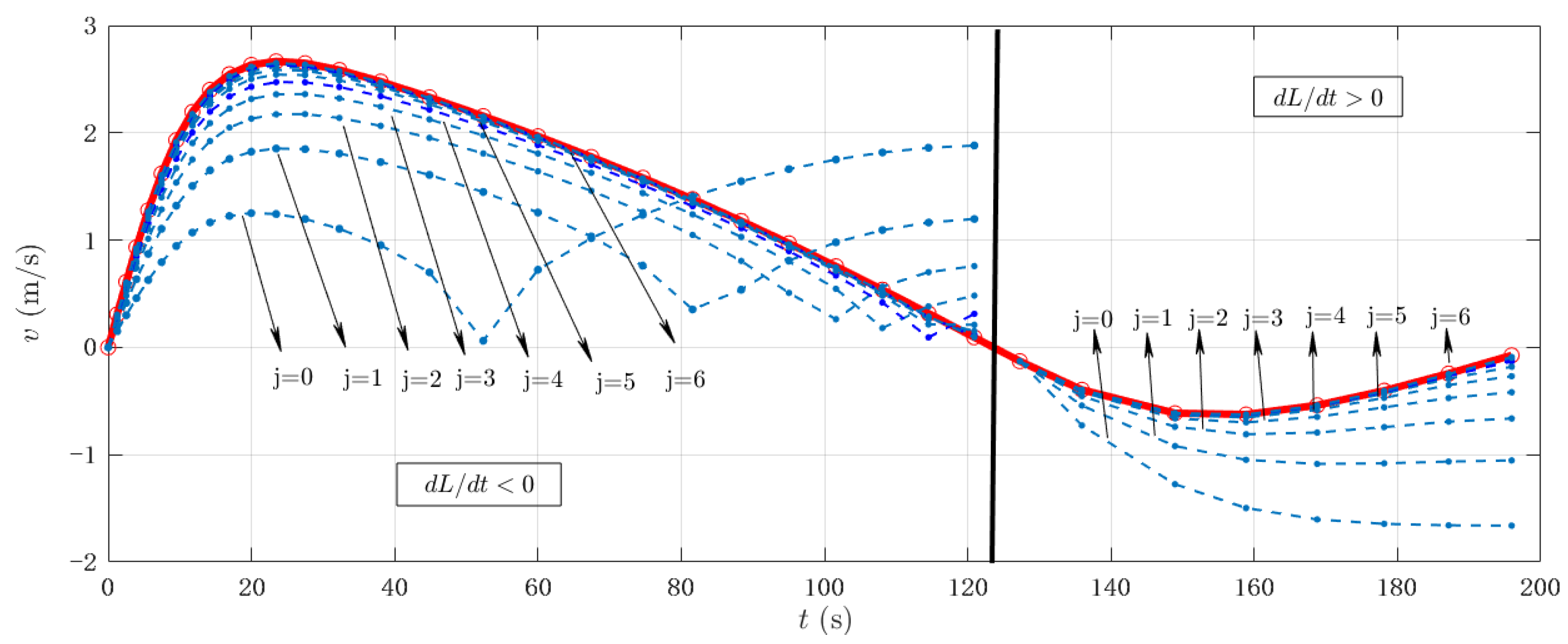
Figure 6 presents the solution considering the first seven terms of the series, expressed explicitly through Equations (29) and (35) for the initial two intervals corresponding to ${\displaystyle \frac{dL}{dt}}\ge 0$ and ${\displaystyle \frac{dL}{dt}}\le 0$, respectively. The results demonstrate rapid convergence of the analytical solution to the numerical solution with relatively few terms.

Furthermore, the analytical model was validated using experimental measurements conducted by the authors, as reported in Reference [5], where a single pipeline with an internal diameter of 42 mm and a total length of 4.36 m was employed. In this case, conditions similar to those of the practical application were considered, implying that the upstream end remained closed during the simulations. For the analysis, the initial air pocket size, $x_0$, ranged from 0.205 to 0.450 m; longitudinal pipe slopes varied between 0.457 and 0.515 rad; and resistance coefficients at the regulating valves ranged from 11.89 to 138.41 × 10⁶ ms²/m⁶. The analytical solution was applied under the assumption of instantaneous valve opening to provide conservative (safety) estimates, while the experiments were conducted considering a gradual valve opening. 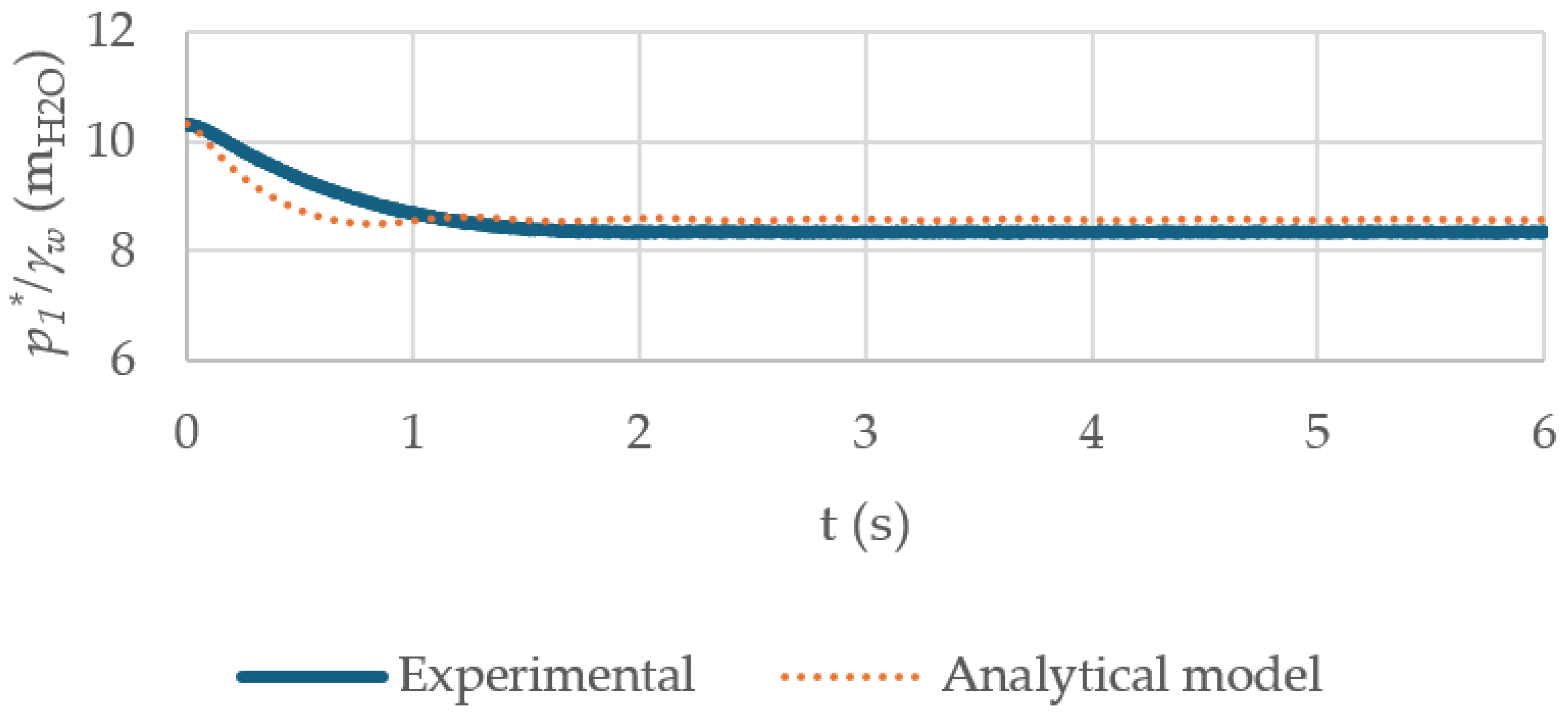Figure 7 presents a comparison between the computed and measured evolution of the air pocket pressure over time, for an initial air pocket volume of 0.450 m, a longitudinal slope of 0.457 rad, and a resistance coefficient of 30.86 × 10⁶ ms²/m⁶. The discrepancy observed during the initial seconds is attributed to the experimental setup, in which the regulating valve was gradually opened using an opening manoeuvre time of 0.3 s.

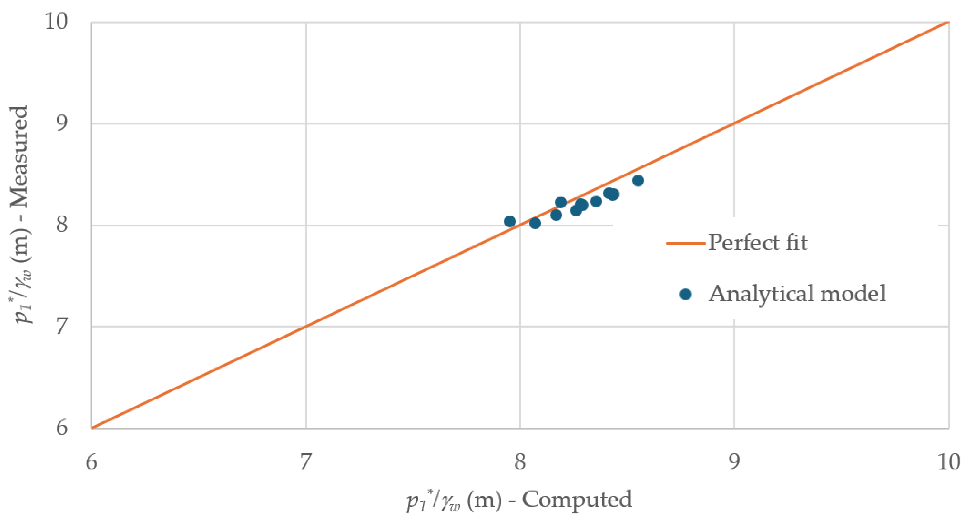
Figure 8 compares the maximum air pocket pressures obtained from 12 measurements, demonstrating that the analytical model can accurately capture these values, which are crucial to detect if a pipeline can have a risk of collapse.

5. Discussion

The original coupled model defined by Equations (4)–(6) has been reduced to a single second-order nonlinear ordinary differential equation in the water column length $L\left(t\right)$ (see Equation (13)). This formulation captures the intrinsic oscillatory dynamics arising from the air–water interface reversal, but the presence of $\left|{\displaystyle \frac{dL}{dt}}\right|$ renders direct integration intractable. By introducing the change of variables $u\left(L\right)={\displaystyle \frac{dL}{dt}}$, it is possible to eliminate the absolute value nonlinearity and recast the problem into the linear first-order ODE for $u^2\left(L\right)$ (see Equation (18)), valid over monotonic segments of ${\displaystyle \frac{dL}{dt}}$. This key transformation not only simplifies the analytical treatment but also yields explicit integral expressions for $u^2\left(L\right)$ in both regimes ${\displaystyle \frac{dL}{dt}}\ge 0$ (see Equations (20)–(22)) and ${\displaystyle \frac{dL}{dt}}\le 0$ (see Equations (32)–(34)).

Constructing the global solution thus requires stitching together these local solutions at the sign change instants $t_k$ (where ${\displaystyle \frac{dL}{dt}}=0$). In this research, the switching times were determined numerically by locating zeros of the water velocity in the reduced model; thereafter, the piecewise integrals were evaluated to produce continuous profiles of $L\left(t\right)$, $v\left(t\right)$, and $p_1^{\ast }\left(t\right)$ (Figure 3, Figure 4 and Figure 5) that agree closely with fully numerical simulations of the original system. Moreover, the series expansions of the special integrals $I_j$ and $F_j$ converge rapidly; even truncating after seven terms recovers the numerical velocity profile almost exactly (Figure 6), demonstrating the practical utility of the analytical analysis.

Although solutions (36)–(38) obtained from (20) and (32) are not explicitly continuous or differentiable for $t\ge 0$ (especially on $t_k$ with $k=0,1,2,\dots$), the fact that both (18) and (31) were derived from (13) ensures that $v\left(t\right)=-{\displaystyle \frac{d^{2}L\left(t\right)}{d{t}^2}}$ is defined globally for $t\ge 0$, and therefore, $v=-{\displaystyle \frac{dL\left(t\right)}{dt}}$ and $L\left(t\right)$ are continuous and differentiable for $t\ge 0$.

On the other hand, the simplified model can be as precise as desired whenever the time subintervals determined by the values $t_k$ with $k=0,1,2,\dots$ are computed correctly depending on the sign of $v\left(t\right)$.

However, there are some errors generated while computing v, L, and $p_1^{\ast }$ from expressions (36)–(38). These errors arise from the truncation of the numerical computations of the integral terms ($A\left(L\right)$, $B_1\left(L\right)$, ${\mathcal{I}}_j$, and $B_2\left(L\right)$) and the series ${\mathcal{F}}_j$. In addition, round-off errors might come up due to hardware architecture and software configuration used for calculations. All these errors can be compensated by selecting an appropriate step size for the time variable.

The proposed model could be further optimised from a physical standpoint by acknowledging that the air–water interface may adopt various configurations—such as bubble flow, plug flow, stratified wave flow, and stratified smooth flow—rather than assuming a strictly vertical profile. These flow regimes are particularly relevant in pipelines with larger diameters or lower longitudinal slopes. Furthermore, the current mathematical model does not account for the effect of air backflow, which may occur especially in largediameter pipes, where air can travel from the regulating valve at the downstream end back towards the upstream end.

Finally, the proposed solution method, which treats the cases in which the velocity changes direction separately, can be generalised to describe oscillations involving dissipative forces proportional to the square (or another even power) of the water velocity but acting in the opposite direction. This approach could be applied to the solution of ordinary differential equations that include sign-changing terms, such as those that involve absolute values of the variable under study.

Water utilities increasingly seek to implement digital twin systems within water distribution networks. As draining processes in pressurised pipelines can potentially lead to pipeline collapse, the proposed analytical solution offers a rapid means of estimating these effects. Real-time data are essential for accurately calibrating the phenomenon under study to establish a reliable digital twin. As physical equations govern the draining process examined in this study, variations in the initial parameters do not affect the model’s applicability. However, the model is specifically designed for drainage operations and unsuitable for filling processes, where different parameters and governing variables come into play.

6. Conclusions

This research has analysed the problem of emptying processes with an entrapped air pocket. The corresponding mathematical model for this physical phenomenon is illustrated at the beginning. Based on this model, this research demonstrated an analytical solution that can be used to describe this problem. The analytical solution can be a practical tool for implementing a digital twin model to predict emptying operations in water distribution systems.

Considering that the emptying process evidences an oscillatory behaviour where the velocity at which the air–water interface moves switches its sign at specific time intervals, a strategy was proposed to simplify the model and determine a closed-form formula for the solution. Thus, by rewriting the problem in terms of a new variable, the problem could be reduced to a linear model for different time intervals, and an analytical solution based on integral terms was constructed for every time interval for the column length, the velocity of the air–water interface, and the pressure in the air pocket. The solution for the velocity was plotted locally at every time interval after evaluating the integral terms in the solution numerically. It was observed that this solution corresponds with the approximated numerical solution, validating the formulation of the analytical solutions. Finally, a series expansion was proposed for the integral terms at every time interval. The plots for the first seven partial summations of the series exhibit the convergence of the solution, demonstrating the correctness of the proposed analytical solution.