
Analysis of the Dynamic Active Earth Pressure from c-φ Backfill Considering the Amplification Effect of Seismic Acceleration


Abstract
1. Introduction
2. Seismic Active Earth Pressure Analysis
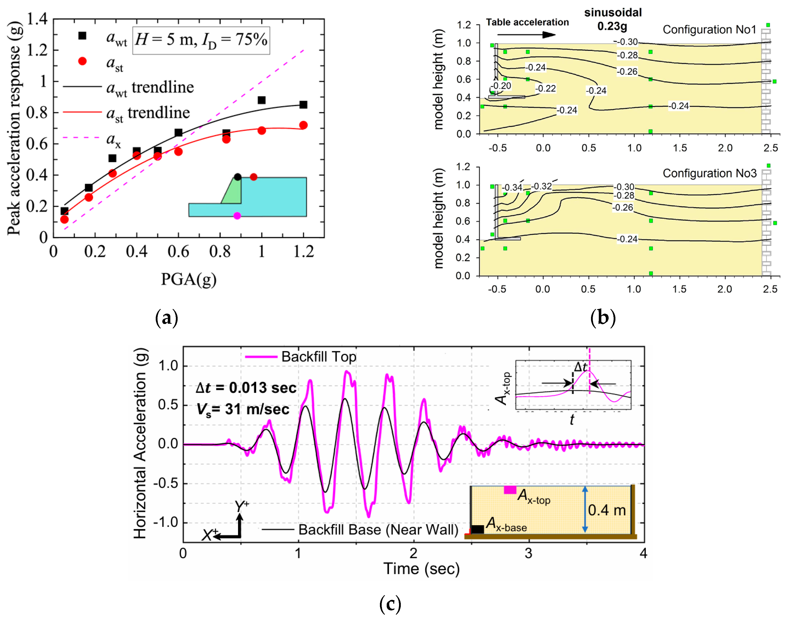
2.1. Acceleration Response Characteristics of the Backfill Behind the Retaining Wall
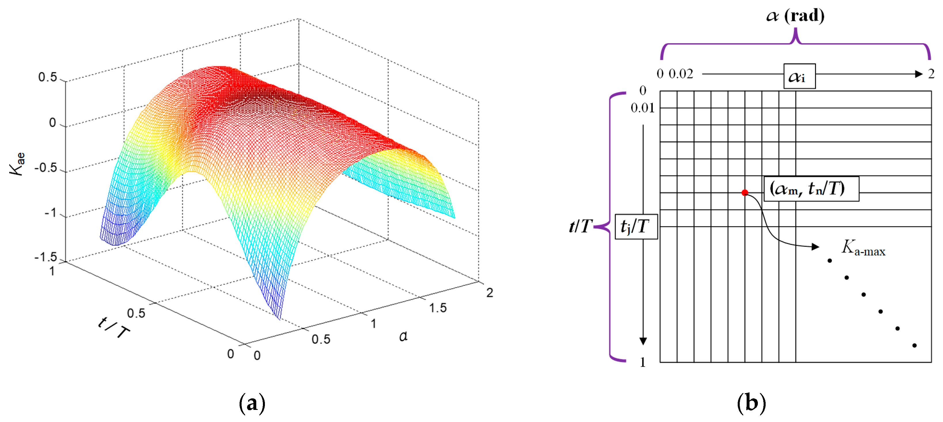
2.2. Analysis of Active Earth Pressure Forces on a Retaining Wall Under Seismic Loading
2.3. Computation of Active Earth Pressure Using the Proposed Calculation Formula
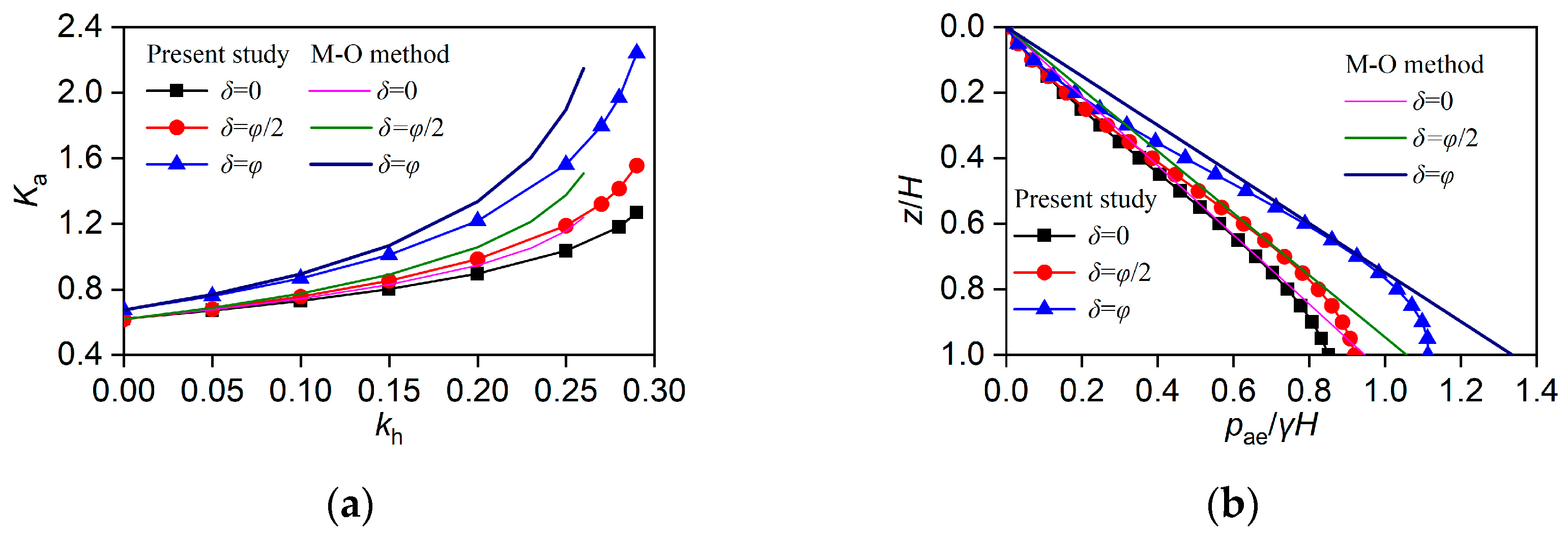
3. Comparison and Validation of the Proposed Calculation Method
3.1. Validation 1
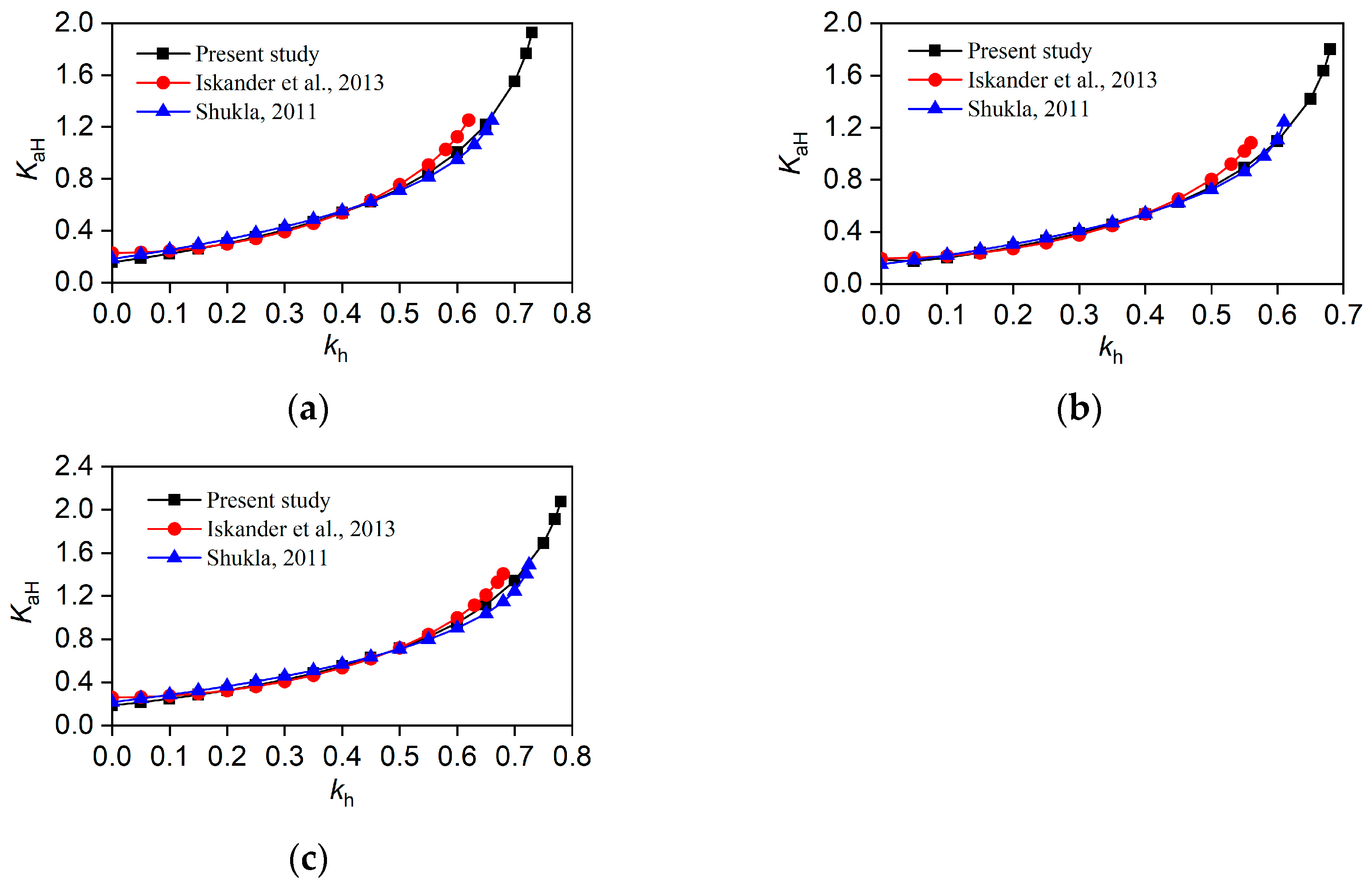
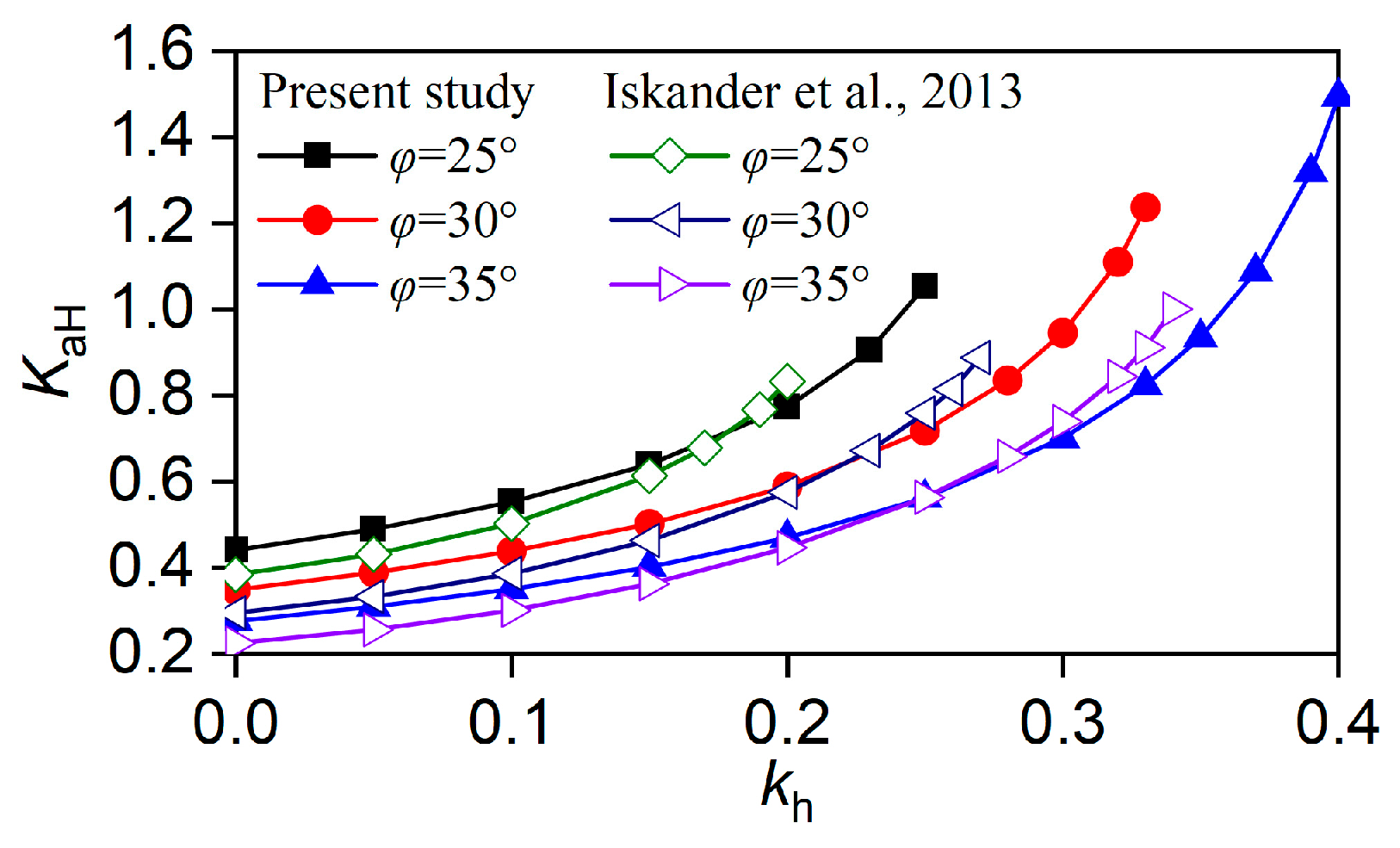
3.2. Validation 2
3.3. Validation 3
4. Parametric Study
4.1. Effect of Acceleration Amplification Factor fa
4.2. Effect of Backfill-Wall Friction Angle δ
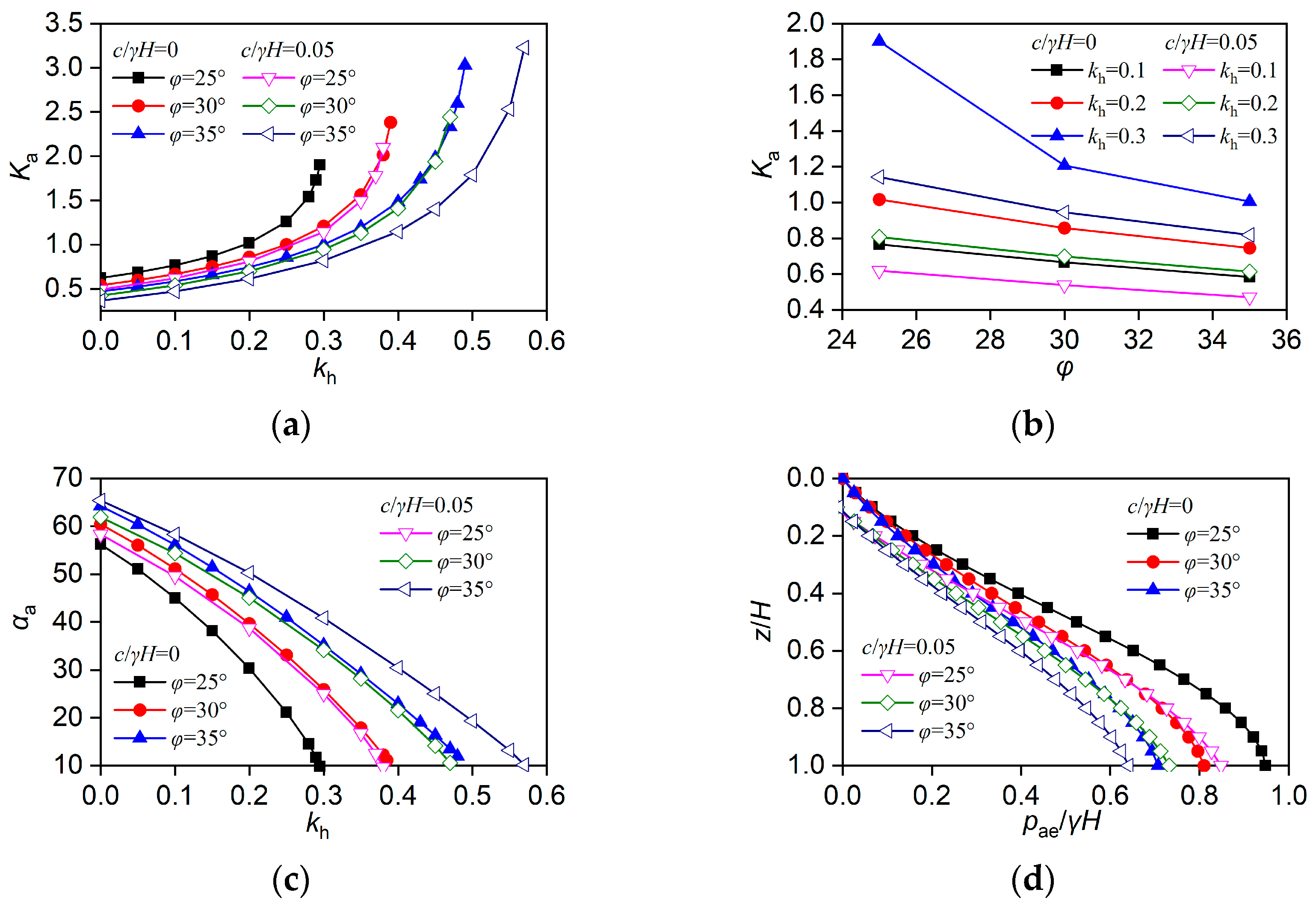
4.3. Effect of Internal Friction Angle φ
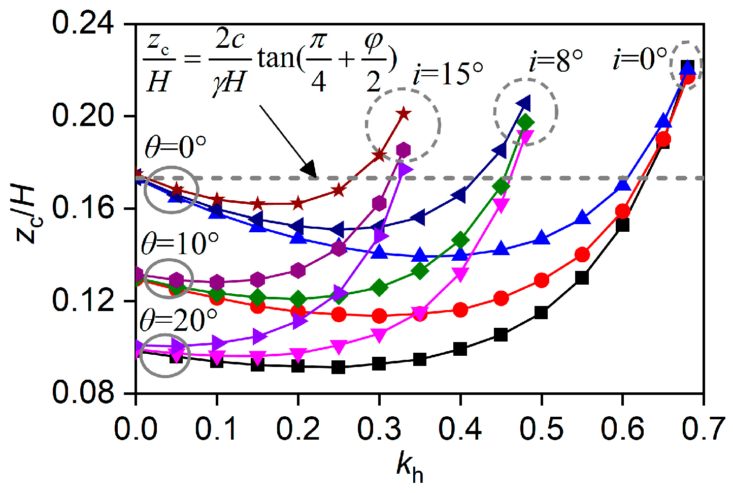
4.4. Effect of Retaining Wall Slope Angle θ
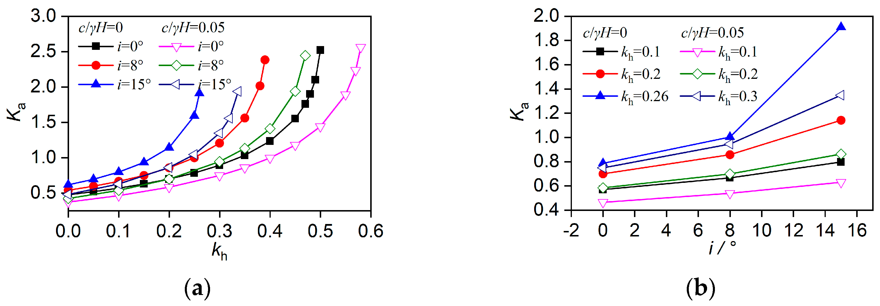
4.5. Effect of Backfill Slope Angle i
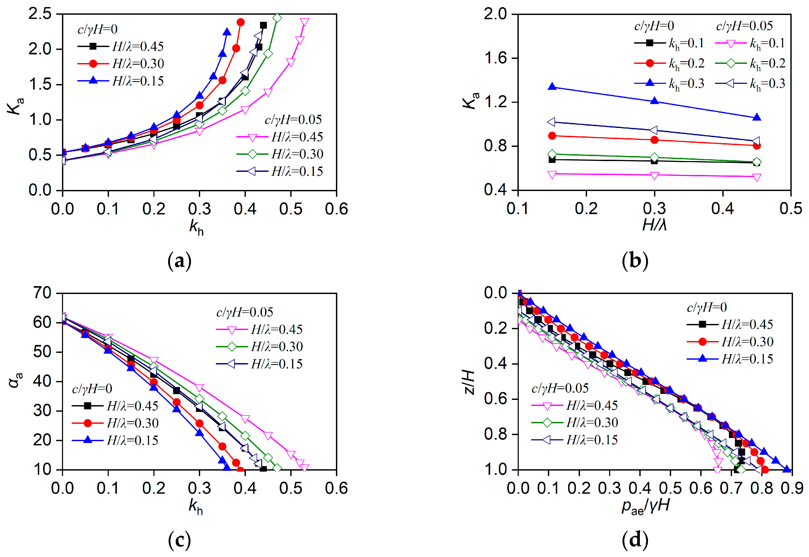
4.6. Effect of Period of Lateral Shaking T
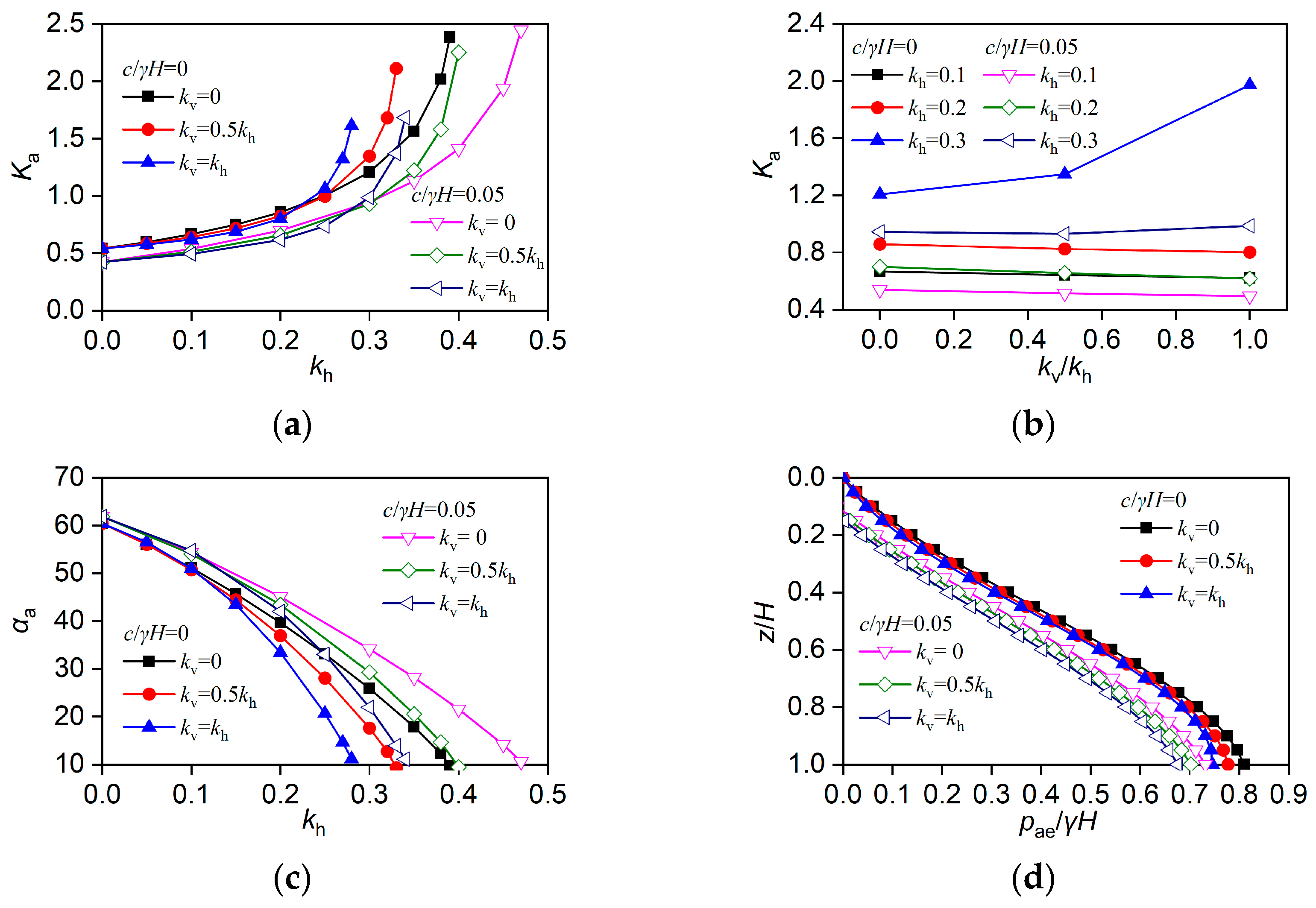
4.7. Effect of Horizontal and Vertical Seismic Acceleration Coefficients kh and kv
4.8. Effect of Normalized Backfill Cohesion c/γH
4.9. Summary
5. Conclusions
Author Contributions
Funding
Institutional Review Board Statement
Informed Consent Statement
Data Availability Statement
Conflicts of Interest
Appendix A. Derivation of the Formulas for the Active Earth Pressure Coefficient and the Distribution of the Active Earth Pressure
Appendix B. Nomenclature
| H | Height of retaining wall |
| θ | Slope angle of the retaining wall |
| α | Angle between the failure surface of the backfill and the horizontal bottom plane |
| i | Backfill slope angle |
| fa | Amplification factor |
| γ | Unit weight of backfill |
| δ | Friction angle between the backfill and the retaining wall |
| kh | Horizontal seismic acceleration coefficient at the base |
| kv | Vertical seismic acceleration coefficient at the base |
| z | Depth from the top of the wall |
| L | Vertical projection of BC |
| ah(z, t) | Horizontal acceleration in the backfill at depth z and time t |
| av(z, t) | Vertical acceleration in the backfill at depth z and time t |
| m(z) | Weight of the slice |
| W | Weight of the failure wedge |
| Qh(t) | Horizontal inertia forces in the active wedge |
| Qv(t) | Vertical inertia forces in the active wedge |
| λ | Wavelength of shear wave |
| η | Wavelength of primary wave. |
| T | Period of lateral shaking |
| ω | Angular frequency of motion = 2π/T |
| Pae(t) | Lateral active force acting on the retaining wall |
| cw | Soil–wall adhesion |
| c | Backfill cohesion |
| φ | Backfill internal friction angle |
| La1 | Effective adhesive length between backfill and wall |
| La2 | Effective length of sliding surface in the backfill |
| zc | Depth of tension crack |
| Ka(t) | Active earth pressure coefficient |
| pae(z, t) | Distribution of active earth pressure on the retaining wall |
References
- Kobayashi, T.; Zen, K.; Yasufuku, N.; Nagase, H.; Chen, G.; Kasama, K.; Hirooka, A.; Wada, H.; Yuji Onoyama, Y.; Uchida, H. Damage to Residential Retaining Walls at the Genkai-Jima Island Induced by the 2005 Fukuoka-Ken Seiho-Oki Earthquake. Soils Found. 2006, 46, 793–804. [Google Scholar] [CrossRef]
- Xiao, S.; Zhang, J.; Ma, Y. Investigation on failure of side-hill gravity retaining walls in regions of the Wenchuan Earthquake. Chin. J. Undergr. Space Eng. 2011, 07, 174–178. (In Chinese) [Google Scholar]
- Okabe, S. General Theory on earth pressure and seismic stability of retaining wall and dam. Proc. Civ. Eng. Soc. 1924, 10, 1277–1323. [Google Scholar]
- Mononobe, N.; Matsho, H. On the determination of earthquake pressure during earthquake. Proc. World Eng. Congr. 1929, 9, 177–185. [Google Scholar]
- Steedman, R.S.; Zeng, X. The influence of phase on the calculation of pseudo-static earth pressure on a retaining wall. Géotechnique 1990, 40, 103–112. [Google Scholar] [CrossRef]
- Zeng, X.; Steedman, R.S. On the behaviour of quay walls in earthquakes. Geotechnique 1993, 43, 417–431. [Google Scholar] [CrossRef]
- Azad, A.; Yasrobi, S.S.; Pak, A. Seismic active pressure distribution history behind rigid retaining walls. Soil Dyn. Earthq. Eng. 2008, 28, 365–375. [Google Scholar] [CrossRef]
- Ghosh, P. Seismic active earth pressure behind a nonvertical retaining wall using pseudo-dynamic analysis. Can. Geotech. J. 2008, 45, 117–123. [Google Scholar] [CrossRef]
- Ghosh, S. Pseudo-dynamic active force and pressure behind battered retaining wall supporting inclined backfill. Soil Dyn. Earthq. Eng. 2010, 30, 1226–1232. [Google Scholar] [CrossRef]
- Choudhury, D.; Katdare, A.D.; Pain, A. New method to compute seismic active earth pressure on retaining wall considering seismic waves. Geotech. Geol. Eng. 2014, 32, 391–402. [Google Scholar] [CrossRef]
- Qin, C.; Chian, S.C. Pseudo-dynamic lateral earth pressures on rigid walls with varying cohesive-frictional backfill. Comput. Geotech. 2020, 119, 103289. [Google Scholar] [CrossRef]
- Luo, W.; Gong, C.; Wang, H.; Yang, X. Estimation of active earth pressure based on pseudo-dynamic approach and discretization technique. J. Cent. South. Univ. 2021, 28, 2890–2904. [Google Scholar] [CrossRef]
- Lei, M.; Li, J.; Zhao, C.; Shi, C.; Yang, W.; Deng, E. Pseudo-dynamic analysis of three-dimensional active earth pressures in cohesive backfills with cracks. Soil Dyn. Earthq. Eng. 2021, 150, 106917. [Google Scholar] [CrossRef]
- Pain, A.; Choudhury, D.; Bhattacharyya, S.K. Seismic rotational stability of gravity retaining walls by modified pseudo-dynamic method. Soil Dyn. Earthq. Eng. 2017, 94, 244–253. [Google Scholar] [CrossRef]
- Fathipour, H.; Safardoost Siahmazgi, A.; Payan, M.; Chenari, R.J.; Veiskarami, M. Evaluation of the active and passive pseudo-dynamic earth pressures using finite element limit analysis and second-order cone programming. Geotech. Geol. Eng. 2023, 41, 1921–1936. [Google Scholar] [CrossRef]
- Kang, X.; Yang, X.; Wu, C. Modified pseudo-dynamic bearing capacity of reinforced soil foundations. Comput. Geotech. 2024, 165, 105901. [Google Scholar] [CrossRef]
- Kumar, M.; Chatterjee, K. Modified pseudo-dynamic based soil-structure interaction of caisson with a novel 3D failure wedge. Comput. Geotech. 2023, 153, 105079. [Google Scholar] [CrossRef]
- Kang, X.; Zhu, J.; Liu, L. Seismic bearing capacity of strip footings with modified pseudo-dynamic method. KSCE J. Civ. Eng. 2024, 28, 1657–1674. [Google Scholar] [CrossRef]
- Nadgouda, K.; Choudhury, D. Combined seismic bearing capacity factor using modified pseudo-dynamic approach. Geotech. Geol. Eng. 2023, 41, 1947–1959. [Google Scholar] [CrossRef]
- Yang, X.; Wei, J. Seismic stability for reinforced 3D slope in unsaturated soils with pseudo-dynamic approach. Comput. Geotech. 2021, 134, 104124. [Google Scholar]
- Zhong, J.; Yang, X. Pseudo-dynamic stability of rock slope considering Hoek–Brown strength criterion. Acta Geotech. 2022, 17, 2481–2494. [Google Scholar] [CrossRef]
- Qin, C.; Chian, S.C. Impact of earthquake characteristics on seismic slope stability using modified pseudo-dynamic method. Int. J. Geomech. 2019, 19, 04019106. [Google Scholar] [CrossRef]
- Zhou, J.; Zheng, Z.; Bao, T.; Tu, X.; Yu, J.; Qin, C. Assessment of rigorous solutions for pseudo-dynamic slope stability: Finite-element limit-analysis modelling. J. Cent. South. Univ. 2023, 30, 2374–2391. [Google Scholar] [CrossRef]
- Wu, X.; Cui, Z.; Yang, B.; Lian, B. Seismic stability of anchored slopes considering tension-shear coupling effect by modified pseudo-dynamic approach. Soil Dyn. Earthq. Eng. 2025, 190, 109206. [Google Scholar] [CrossRef]
- Qin, C.; Chian, S.C. Kinematic analysis of seismic slope stability with a discretisation technique and pseudo-dynamic approach: A new perspective. Géotechnique 2018, 68, 492–503. [Google Scholar] [CrossRef]
- Singh, P.; Bhartiya, P.; Chakraborty, T.; Basu, D. Numerical investigation and estimation of active earth thrust on gravity retaining walls under seismic excitation. Soil Dyn. Earthq. Eng. 2023, 167, 107798. [Google Scholar] [CrossRef]
- Kloukinas, P.; di Santolo, A.S.; Penna, A.; Dietz, M.; Evangelista, A.; Simonelli, A.L.; Taylor, C.; Mylonakis, G. Investigation of seismic response of cantilever retaining walls: Limit analysis vs shaking table testing. Soil Dyn. Earthq. Eng. 2015, 77, 432–445. [Google Scholar] [CrossRef]
- Tiwari, R.; Lam, N. Displacement based seismic assessment of base restrained retaining walls. Acta Geotech. 2022, 17, 3675–3694. [Google Scholar] [CrossRef]
- Jo, S.B.; Ha, J.G.; Lee, J.S.; Kim, D.S. Evaluation of the seismic earth pressure for inverted T-shape stiff retaining wall in cohesionless soils via dynamic centrifuge. Soil Dyn. Earthq. Eng. 2017, 92, 345–357. [Google Scholar] [CrossRef]
- Kim, K.; Khalifa, M.A.; El Naggar, M.H.; Elgamal, A. Seismic performance of U-shaped spillway retaining wall from shake table tests. Soil Dyn. Earthq. Eng. 2023, 172, 108020. [Google Scholar] [CrossRef]
- He, H.; Payan, M.; Senetakis, K. The behaviour of a recy cled road base aggregate and quartz sand with bender/extender element tests under variable stress states. Eur. J. Env. Civ. Eng. 2021, 25, 152–169. [Google Scholar] [CrossRef]
- Payan, M.; Khoshini, M.; Jamshidi Chenari, R. Elastic dynamic young’s modulus and poisson’s ratio of sand silt mixtures. J. Mater. Civ. Eng. 2020, 32, 04019314. [Google Scholar] [CrossRef]
- Iskander, M.; Chen, Z.; Omidvar, M.; Guzman, I.; Elsherif, O. Active static and seismic earth pressure for c–φ soils. Soils Found. 2013, 53, 639–652. [Google Scholar] [CrossRef]
- Shukla, S.J. Dynamic active thrust from c–φ soil backfills. Soil Dyn. Earthq. Eng. 2011, 31, 526–529. [Google Scholar] [CrossRef]
- Nakajima, S.; Ozaki, T.; Sanagawa, T. 1 g Shaking table model tests on seismic active earth pressure acting on retaining wall with cohesive backfill soil. Soils Found. 2021, 61, 1251–1272. [Google Scholar] [CrossRef]
- Terzaghi, K.; Peck, R.B.; Mesri, G. Soil Mechanics in Engineering Practice, 3rd ed.; John Wiley & Sons: New York, NY, USA, 1996. [Google Scholar]


| Backfill | Unit Weight of Backfill | Residual Strength | |||
|---|---|---|---|---|---|
| φres | cres | c/γh | |||
| Case 3 | Inagi sand, w = 12% | 15.6 kN/m3 | 32.5° | 2.2 kPa | 0.24 |
| Case 4 | Inagi sand, w = 0% | 13.6 kN/m3 | 39° | 0 kPa | 0 |
| ID | fa | δ/° | φ/° | θ/° | i/° | H/λ | kv/kh | c/γH |
|---|---|---|---|---|---|---|---|---|
| 1 | 1.0, 1.4, 1.8 | 15 | 30 | 20 | 8 | 0.30 | 0 | 0, 0.05 |
| 2 | 1.0 | 0, 15, 30 | 30 | 20 | 15 | 0.30 | 0 | 0, 0.05 |
| 3 | 1.4 | 15 | 25, 30, 35 | 20 | 8 | 0.30 | 0 | 0, 0.05 |
| 4 | 1.4 | 15 | 30 | −20, 0, 20 | 8 | 0.30 | 0 | 0, 0.05 |
| 5 | 1.4 | 15 | 30 | 20 | 0, 8, 15 | 0.30 | 0 | 0, 0.05 |
| 6 | 1.4 | 15 | 30 | 20 | 8 | 0.45, 0.30, 0.15 | 0 | 0, 0.05 |
| 7 | 1.4 | 15 | 30 | 20 | 8 | 0.30 | 0, 0.5, 1.0 | 0, 0.05 |
| fa | δ | φ | θ | i | T | kh | kv | c/γH | |
|---|---|---|---|---|---|---|---|---|---|
| Ka | ↑ | ↑ | ↓ | ↑ | ↑ | ↑ | ↑ | * | ↓ |
| αa | ↓ | ↓ | ↑ | ↑ | ↓ | ↓ | ↓ | ↓ | ↑ |
Disclaimer/Publisher’s Note: The statements, opinions and data contained in all publications are solely those of the individual author(s) and contributor(s) and not of MDPI and/or the editor(s). MDPI and/or the editor(s) disclaim responsibility for any injury to people or property resulting from any ideas, methods, instructions or products referred to in the content. |
© 2025 by the authors. Licensee MDPI, Basel, Switzerland. This article is an open access article distributed under the terms and conditions of the Creative Commons Attribution (CC BY) license (https://creativecommons.org/licenses/by/4.0/).
Share and Cite
Sun, Z.; Wang, W.; Liu, H. Analysis of the Dynamic Active Earth Pressure from c-φ Backfill Considering the Amplification Effect of Seismic Acceleration. Appl. Sci. 2025, 15, 5966. https://doi.org/10.3390/app15115966
Sun Z, Wang W, Liu H. Analysis of the Dynamic Active Earth Pressure from c-φ Backfill Considering the Amplification Effect of Seismic Acceleration. Applied Sciences. 2025; 15(11):5966. https://doi.org/10.3390/app15115966
Chicago/Turabian StyleSun, Zhiliang, Wei Wang, and Hanghang Liu. 2025. "Analysis of the Dynamic Active Earth Pressure from c-φ Backfill Considering the Amplification Effect of Seismic Acceleration" Applied Sciences 15, no. 11: 5966. https://doi.org/10.3390/app15115966
APA StyleSun, Z., Wang, W., & Liu, H. (2025). Analysis of the Dynamic Active Earth Pressure from c-φ Backfill Considering the Amplification Effect of Seismic Acceleration. Applied Sciences, 15(11), 5966. https://doi.org/10.3390/app15115966