Whole-Body Motion Generation for Balancing of Biped Robot

Abstract

A humanoid robot has a similar form to humans, allowing it to be deployed directly into many existing infrastructures built for people, making it highly applicable to future industries or services. However, generating motion is challenging, and it is highly affected by disturbances due to its complex dynamic characteristics. This paper proposes a method to enable a biped robot to achieve stable motion in various environments. The capture point (CP) control is used to modify the zero moment point (ZMP) to stabilize the naturally divergent dynamics of the simplified linear inverted pendulum model (LIPM) and a model predictive control (MPC) framework is implemented to generate a center of mass (COM) trajectory that tracks the adjusted ZMP. To minimize angular momentum caused by disturbances and discrepancies between the actual robot and the dynamics model, arm motion is generated through a momentum controller. Various walking simulations were conducted to verify stable whole-body motion.

1. Introduction

Humanoids, similar to humans, can be utilized in various fields [1] and are increasingly accepted in public services [2,3], replacing humans in existing social infrastructures. Humanoids need to perform tasks across a wide range of areas that other types of robots are not expected to handle. Since the dynamics of humanoid robots are highly complex, motion planning and control are particularly challenging [4,5].

Since deriving the dynamic equations of humanoid robots is highly complex, and utilizing them in motion planning and control is very challenging, simplified models have often been used. One widely used simplified model is the linear inverted pendulum model (LIPM), where the robot is represented as a single mass, and a support point called the zero moment point (ZMP) is fixed to describe the robot’s motion [6]. Although LIPM can easily generate the trajectory of the center of mass (COM), there exist differences in dynamics between the model and actual robots. To minimize the differences, the gravity-compensated inverted pendulum model (GCIPM) was introduced in [7], which incorporates the dynamics of the swinging leg ignored by LIPM. To reduce the model differences further, the dual linear inverted pendulum model (D-LIPM) was introduced, which splits the model into horizontal and vertical components while avoiding the complexity of nonlinear models [8].

Nonetheless, discrepancies between simplified models and actual robots, along with external disturbances, often cause instability during motion. To mitigate this, ZMP tracking controllers have been developed to minimize these inconsistencies. In [9], a linear quadratic optimal controller was used for ZMP feedback control. In [10], a preview controller was designed based on a future reference ZMP. The form of the preview controller is similar to that of model predictive control (MPC). In the field of robot control, MPC has been widely researched over the past decade. By reflecting the current state and replanning the motion of the robot at each step, it can make the robot more robust to disturbances [11]. In [12], the ZMP preview controller was improved by designing a linear model predictive control (LMPC), avoiding nonlinearity, taking advantage of shorter computation times, and tracking the reference ZMP even in the presence of disturbances. LMPC has extended to vertical motion and successfully replicated movements similar to human walking [13].

However, control strategies that simply track the ZMP have limitations in maintaining balance when walking under large disturbances or on uneven terrain, unless the ZMP is modified. To overcome the limitations of fixed ZMP tracking, the concept of the capture point (CP) was adopted to predict and stabilize the motion of biped robots under disturbance. CP was initially proposed in the context of representing the region on the ground where a robot has to take a step to come to a complete stop without falling [14] and is mathematically equivalent to other formulations such as the extrapolated center of mass (XCoM) [15] and the divergent component of motion (DCM) [16]. These concepts share the goal of capturing the divergent nature of bipedal dynamics and have been widely adopted in balance control and motion planning.

CP not only reflects the instantaneous state of the COM but also enables a structural decomposition of the second-order LIPM dynamics into two first-order systems: one is a stable system in which the COM follows the CP, and the other is a naturally unstable system in which the CP is driven by the ZMP. This structure allows efficient stabilization by controlling only the unstable part. Since CP dynamics are inherently divergent and driven by ZMP, stabilizing CP effectively modifies the ZMP. In [17], a simple method was proposed to generate the COM trajectory that is more robust against disturbances by adjusting the ZMP based on the CP concept. In [18], CP tracking and a CP end-of-step controller were designed to stabilize the dynamics of the LIPM by modifying the reference ZMP. In [19], push recovery was implemented through optimization based on the analytical solution of the CP concept.

Depending on how the optimization problem is formulated, MPC can be applied to modify the ZMP [20]. A cascaded structure combining CP control with MPC allows for robust walking control, where the CP feedback stabilizes the divergent dynamics and adjusts ZMP, MPC generates feasible COM trajectories based on the adjusted ZMP. In [21], the DCM concept was utilized along with a single MPC that combines ZMP manipulation, footstep adjustment, and centroidal moment pivot (CMP) modulation, enabling robust walking on irregular terrain. In [22], the ZMP modification through CP control from [18] was combined with the modified LMPC approach used in [20] to maintain balance in the presence of disturbances.

Despite these advancements, most previous works neglect angular momentum. Angular momentum plays an essential role in enhancing the balance of a walking humanoid. However, most studies assume a point mass model without consideration of angular momentum. The upper body of a humanoid robot usually takes a large proportion of momentum due to its dominant inertia proportion [23]. In [24,25], the momentum equations were expressed in a linear form, and resolved momentum control was proposed to modify the movements of the body and free joints to track the reference momentum. In [26], inverse dynamics were used to generate upper body rotation for balance maintenance. In [27], the angular momentum generated by the lower body movements was calculated to compensate for it using the upper body, compensating for the yaw direction angular momentum. However, existing studies still have limitations in flexibly responding to unexpected disturbances or adjusting balance using the arms, as humans do.

Research on enhancing dynamic stability using robot arms has been pursued through various approaches. Some studies have focused on imitating human arm motions or learning their characteristics based on motion capture [28,29]. Other works have involved maintaining balance through reactive upper-body movements within a whole-body momentum control framework [26], and studies have also explored planning predictive arm responses to disturbances using model hierarchy predictive control (MHPC) [30]. However, these approaches often utilize arm motions as a secondary consequence of specific tasks or complex integrated control systems. The method proposed in this paper generates arm motions in real time through an optimization-based, decoupled momentum controller designed specifically to minimize whole-body angular momentum. This approach establishes a direct objective for angular momentum management and proposes a decoupled framework for arm motion generation, which can enhance the generality and flexibility of application.

In this paper, we propose an arm motion generation through an optimization-based momentum controller. Unlike the lower limbs, the arms of a humanoid robot are not constrained by ground contact, making them particularly suitable for generating compensatory angular momentum. This characteristic becomes especially critical when footstep adjustment is limited or infeasible. Building upon this idea, we propose a whole-body motion generation framework that integrates CP control, MPC, and an optimization-based momentum controller for arm motion. This integrated approach directly addresses the limitations of conventional lower-body-centric control frameworks. These frameworks often struggle with effective angular momentum management, particularly when facing unexpected disturbances or constraints on foot placement. The CP was used to modify the pre-planned ZMP in order to stabilize the dynamics of LIPM. To track the modified ZMP and generate the COM trajectory, MPC was used. While inheriting the CP and MPC structure, our approach extends it by incorporating a decoupled arm control module based on angular momentum minimization. This is achieved by introducing an optimization-based momentum controller that actively utilizes the unconstrained degrees of freedom of the robot, particularly those of the arms. This controller is designed to minimize whole-body angular momentum, thereby generating compensatory motions that enhance overall balance and postural stability. The proposed framework was validated through simulations, with changes in the stride and the step period, as well as unexpected obstacles. The main contributions of this paper are as follows:

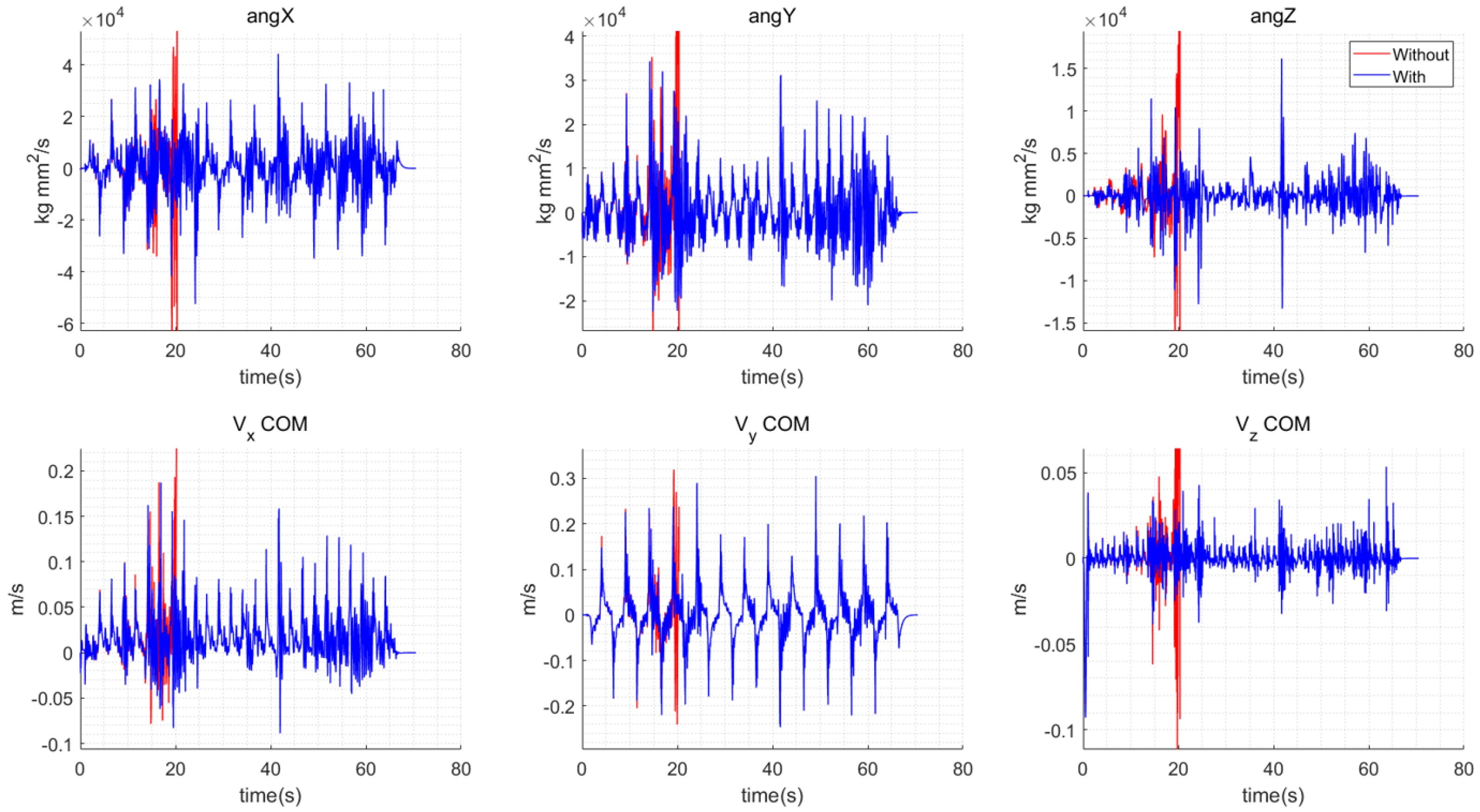
• A novel method for generating arm motions via optimization, designed to minimize whole-body angular momentum and improve balance in the presence of disturbances.
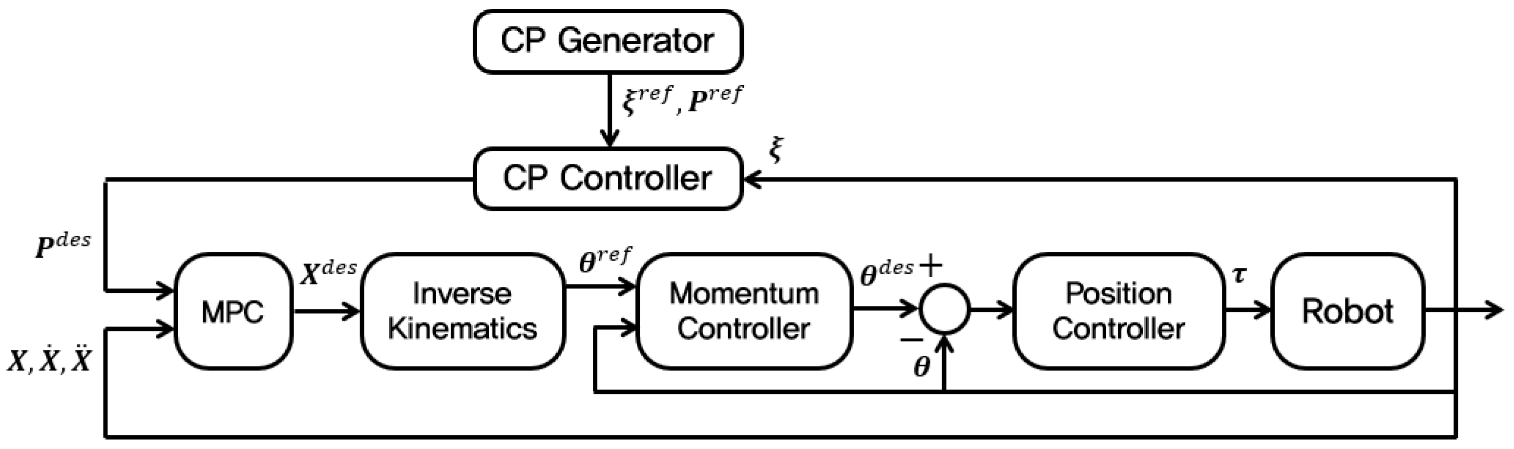
• An integrated whole-body motion generation framework that combines CP control, MPC, and momentum control. This extended and unified modular design improves stability and adaptability, particularly where lower-body-only control is insufficient.

The remainder of this paper is as follows. Section 2 covers the method for walking pattern generation. Section 3 explains how to generate the COM trajectory with an MPC, and Section 4 explains how arm motions are generated with optimization. Section 5 validates the overall algorithm with various simulations, and the conclusion is presented in Section 6.

2. Walking Pattern Generation

The behavior of a biped robot is generally realized by tracking the pre-planned footstep positions of the robot. In this paper, a robot model described by LIPM was used. The fixed footstep positions were given and used as the ZMP.

2.1. Linear Inverted Pendulum Model

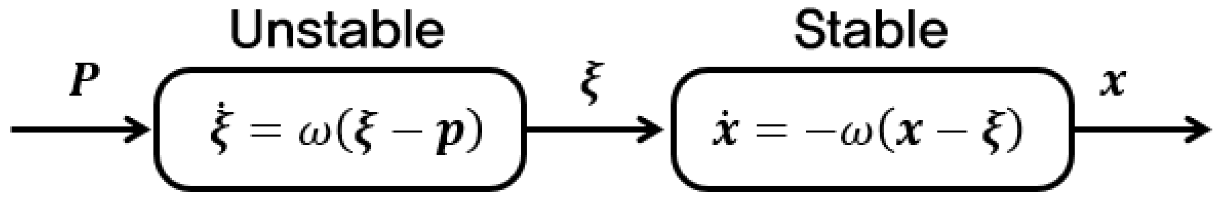
Since the dynamics of a biped robot are very complex, the LIPM is widely used due to its simplicity. In the LIPM, a robot is represented by a single mass point, as shown in Figure 1. It is assumed that the position of the supporting foot is fixed at the ZMP on the ground.

The angular momentum of a point mass m located at the COM, $\mathit{X}\triangleq {\left[xyz\right]}^{\mathrm{T}}$, about the ZMP at ${\mathit{X}}_{ZMP}={\left[p_x{p}_{y}0\right]}^{\mathrm{T}}$ under the influence of gravity is expressed as:

$$\begin{array}{c}\hfill \left[\begin{array}{c}x-p_x\\ y-p_y\\ z\end{array}\right]\times m\left[\begin{array}{c}\ddot{x}\\ \ddot{y}\\ \ddot{z}\end{array}\right]-\left[\begin{array}{c}x-p_x\\ y-p_y\\ z\end{array}\right]\times m\left[\begin{array}{c}0\\ 0\\ -g\end{array}\right]=0\end{array}$$

(1)

Under the assumption that z remains constant at $z_0$, and with $\omega =\sqrt{g/z_0}$, Equation (1) can be simplified:

$$\begin{array}{c}\hfill \ddot{x}={\omega }^2\left(x-p_x\right)\end{array}$$

(2a)

$$\begin{array}{c}\hfill \ddot{y}={\omega }^2\left(y-p_y\right)\end{array}$$

(2b)

With an initial condition of $\mathit{X}\left(t\right)\triangleq {\left[x_0{y}_0{z}_0\right]}^{\mathrm{T}}$ and $\dot{\mathit{X}}\left(t\right)\triangleq {\left[{\dot{x}}_0{\dot{y}}_{0}0\right]}^{\mathrm{T}}$ at $t=0$, the solutions for Equations (2a) and (2b) are:

$$\begin{array}{cc}\hfill x\left(t\right)& \hfill ={\displaystyle \frac{1}{2}}\left[\left(x_0-p_x+{\displaystyle \frac{{\dot{x}}_0}{\omega }}\right)e^{\omega t}+\left(x_0-p_x-{\displaystyle \frac{{\dot{x}}_0}{\omega }}\right)e^{-\omega t}\right]+p_x\hfill \end{array}$$

(3a)

$$\begin{array}{cc}\hfill y\left(t\right)& \hfill ={\displaystyle \frac{1}{2}}\left[\left(y_0-p_y+{\displaystyle \frac{{\dot{y}}_0}{\omega }}\right)e^{\omega t}+\left(y_0-p_y-{\displaystyle \frac{{\dot{y}}_0}{\omega }}\right)e^{-\omega t}\right]+p_y\hfill \end{array}$$

(3b)

In each of Equations (3a) and (3b), there is a term that converges to zero as $t\to \infty$ and a term that diverges to infinity as $t\to \infty$. The latter is called the divergent component.

2.2. Capture Point

In this paper, the concept of CP was used to stabilize the divergent component of LIPM dynamics. Related to this, the DCM [16] or CP [14] is defined by:

$$\begin{array}{c}\hfill {\xi }_x\left(t\right):=x\left(t\right)+{\displaystyle \frac{1}{\omega }}\dot{x}\left(t\right)\end{array}$$

(4)

Using Equations (2a) and (4),

$$\begin{array}{c}\hfill {\xi }_x\left(t\right)=\left(x_0-p_x+{\displaystyle \frac{\dot{x_0}}{\omega }}\right)e^{\omega t}+p_x\end{array}$$

(5)

Differentiating Equation (4) with respect to time, and considering Equations (2a) and (4),

$$\begin{array}{c}\hfill {\displaystyle \frac{d}{dt}}\left({\xi }_x\left(t\right)\right)=\dot{x}\left(t\right)+{\displaystyle \frac{1}{\omega }}\ddot{x}\left(t\right)=\dot{x}\left(t\right)+\omega \left(x\left(t\right)-p_x\right)=\omega ({\xi }_x\left(t\right)-p_x)\end{array}$$

(6)

The CP can be simply expressed in term of constant $p_x$ by solving Equation (6) with initial condition ${\xi }_{x,0}$:

$$\begin{array}{c}\hfill {\xi }_x\left(t\right)=\left({\xi }_{x,0}-p_x\right)e^{\omega t}+p_x\end{array}$$

Since the form of the equation is the same for the y-axis, the expression for the CP, with the constant ZMP $\mathit{P}={\left[p_x{p}_y\right]}^{\mathrm{T}}$ and initial condition ${\mathsf{\xi }}_0\triangleq {\left[{\xi }_{x,0}{\xi }_{y,0}\right]}^{\mathrm{T}}$ is:

$$\begin{array}{c}\hfill \mathsf{\xi }\left(t\right)\triangleq \left[\begin{array}{c}{\xi }_x\left(t\right)\\ {\xi }_y\left(t\right)\end{array}\right]=\left({\mathsf{\xi }}_0-\mathit{P}\right)e^{\omega t}+\mathit{P}\end{array}$$

(7)

The significance of CP lies in its ability to decouple the second-order dynamics of the LIPM. By defining the CP, the LIPM dynamics can be reformulated as two cascaded first-order systems, as shown in Figure 2. Stabilizing the naturally divergent CP dynamics by appropriately modulating the ZMP is crucial for achieving stable COM motion.

2.3. Capture Point Reference Generation for Constant ZMP

Given the predefined footstep locations of ${\mathit{P}}_0^{ref},{\mathit{P}}_1^{ref},\dots ,{\mathit{P}}_N^{ref}$, which are the reference ZMP, and their respective time intervals (step periods) of $T_0,T_1,\dots ,T_N$, the CP reference trajectory for the i-th step is obtained with the backward calculation method [31].

For the i-th step, with CP at the end, denoted by ${\mathsf{\xi }}_{i,end}^{ref}$, can be obtained with Equation (7):

$$\begin{array}{c}\hfill {\mathsf{\xi }}_{i,end}^{ref}={\mathit{P}}_i^{ref}+\left({\mathsf{\xi }}_{i,ini}^{ref}-{\mathit{P}}_i^{ref}\right)e^{\omega T_i}\end{array}$$

(8)

Moreover, since the start of the i-th step is the end of the $(i-1)$-th step, by Equation (8):

$$\begin{array}{c}\hfill {\mathsf{\xi }}_{i,ini}^{ref}={\mathit{P}}_i^{ref}+\left({\mathsf{\xi }}_{i,end}^{ref}-{\mathit{P}}_i^{ref}\right)e^{-\omega T_i}={\mathsf{\xi }}_{i-1,end}^{ref}\end{array}$$

(9)

When the motion stops at the N-th step, the final CP of the $(N-1)$-th step is the same as the N-th ZMP, ${\mathsf{\xi }}_{N-1,end}^{ref}={\mathit{P}}_N^{ref}$. Using Equation (9), the initial and end positions of the CP position for every step are obtained through backward calculations:

$$\begin{array}{c}\hfill \begin{array}{cc}\hfill {\mathsf{\xi }}_{N-1,end}^{ref}& ={\mathit{P}}_N^{ref}\hfill \\ \hfill {\mathsf{\xi }}_{N-1,ini}^{ref}& ={\mathit{P}}_{N-1}^{ref}+\left({\mathsf{\xi }}_{N-1,end}^{ref}-{\mathit{P}}_{N-1}^{ref}\right)e^{-\omega T_{N-1}}={\mathsf{\xi }}_{N-2,end}^{ref}\hfill \\ \hfill {\mathsf{\xi }}_{N-2,ini}^{ref}& ={\mathit{P}}_{N-2}^{ref}+\left({\mathsf{\xi }}_{N-2,end}^{ref}-{\mathit{P}}_{N-2}^{ref}\right)e^{-\omega T_{N-2}}={\mathsf{\xi }}_{N-3,end}^{ref}\hfill \\ \hfill & ⋮\hfill \\ \hfill {\mathsf{\xi }}_{1,ini}^{ref}& ={\mathit{P}}_1^{ref}+\left({\mathsf{\xi }}_{1,end}^{ref}-{\mathit{P}}_1^{ref}\right)e^{-\omega T_{N-2}}={\mathsf{\xi }}_{0,end}^{ref}\hfill \\ \hfill {\mathsf{\xi }}_{ini,0}^{ref}& ={\mathit{P}}_0^{ref}+\left({\mathsf{\xi }}_{end,0}^{ref}-{\mathit{P}}_0^{ref}\right)e^{-\omega T_0}\hfill \end{array}\end{array}$$

(10)

The CP reference as a function of time in the i-th step can be calculated by substituting the initial conditions for each step from Equation (10) to Equation (7):

$$\begin{array}{c}\hfill \mathsf{\xi }{\left(t\right)}_i^{ref}={\left[\begin{array}{c}{\xi }_x\left(t\right)\\ {\xi }_y\left(t\right)\end{array}\right]}_i^{ref}={\mathit{P}}_i^{ref}+\left({\mathsf{\xi }}_{i,ini}^{ref}-{\mathit{P}}_i^{ref}\right)e^{\omega t}\end{array}$$

(11)

3. Generation of COM Trajectory

In this paper, the COM trajectory is generated based on a modified ZMP, which is adjusted through CP control. By stabilizing the divergent dynamics of the LIPM, the CP control modifies the ZMP. The resulting modified ZMP reference, ${\mathit{P}}^{des}$, is then used in an MPC framework to generate COM trajectories.

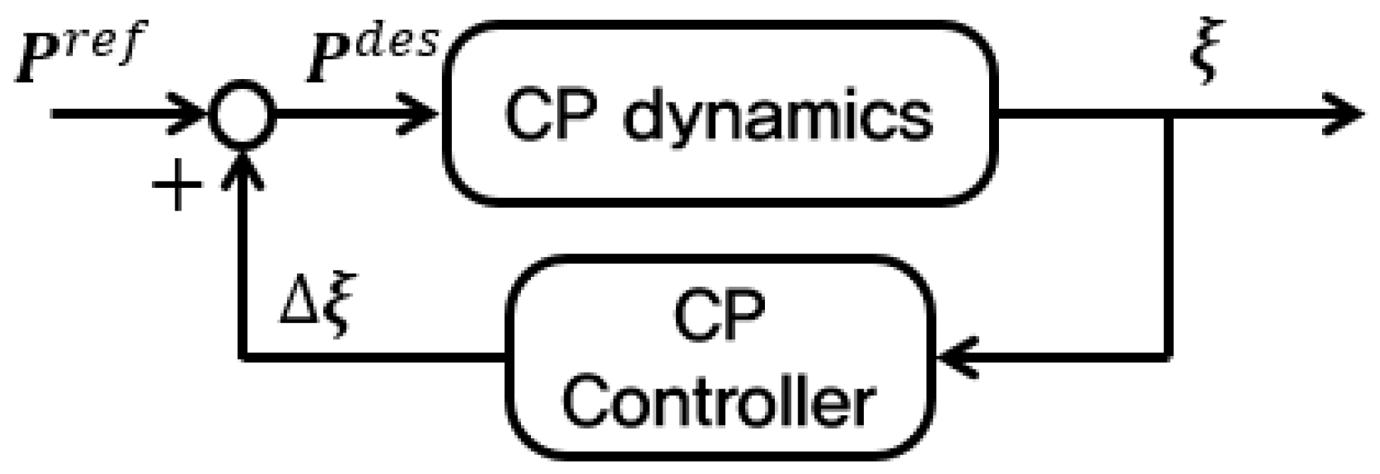
3.1. ZMP Modification Through CP Control

As discussed in Section 2.2, the CP provides a framework for understanding and controlling bipedal locomotion by decomposing the LIPM dynamics. Stabilizing these divergent CP dynamics is crucial because an unstable CP inevitably leads to an unstable COM and potential loss of balance. Therefore, instead of simply tracking a pre-planned ZMP, dynamically modifying the ZMP based on CP feedback allows the robot to better respond to disturbances and maintain stability.

The CP dynamics described by Equation (7) and the COM dynamics described by Equation (4) are in a cascaded form, as shown in Figure 3. Since $\omega$ is a positive constant, the CP dynamics are naturally unstable. If the CP dynamics are controlled to be stable, the COM dynamics will naturally become stable. To stabilize the CP dynamics, the control rule is defined based on error dynamics. This type of error dynamics is well-established in CP-based control for achieving asymptotic stability [32]:

$$\begin{array}{c}\hfill ▵\dot{\mathsf{\xi }}=k_{cp}▵\mathsf{\xi }\end{array}$$

(12)

where $▵\mathsf{\xi }=\mathsf{\xi }-{\mathsf{\xi }}^{ref}$ and $▵\dot{\mathsf{\xi }}={\displaystyle \frac{d}{dt}}\left(▵\mathsf{\xi }\right)$. From Equation (6) with $▵\mathit{P}={\mathit{P}}^{des}-{\mathit{P}}^{ref}$,

$$\begin{array}{c}\hfill ▵\dot{\mathsf{\xi }}=\omega (▵\mathsf{\xi }-▵\mathit{P})\end{array}$$

(13)

by Equations (12) and (13),

$$\begin{array}{c}▵\mathit{P}=▵\mathsf{\xi }-{\displaystyle \frac{1}{\omega }}▵\dot{\mathsf{\xi }}=▵\mathsf{\xi }-{\displaystyle \frac{k_{cp}▵\mathsf{\xi }}{\omega }}\end{array}$$

(14)

$$\begin{array}{c}{\mathit{P}}^{des}={\mathit{P}}^{ref}+\left(1-{\displaystyle \frac{k_{cp}}{\omega }}\right)▵\mathsf{\xi }\end{array}$$

(15)

For $k_{cp}<0$, $▵\mathsf{\xi }\to 0$ as $t\to \infty$ by the control rule (12). The ZMP is modified through CP control, which enables the naturally diverging CP to track its reference.

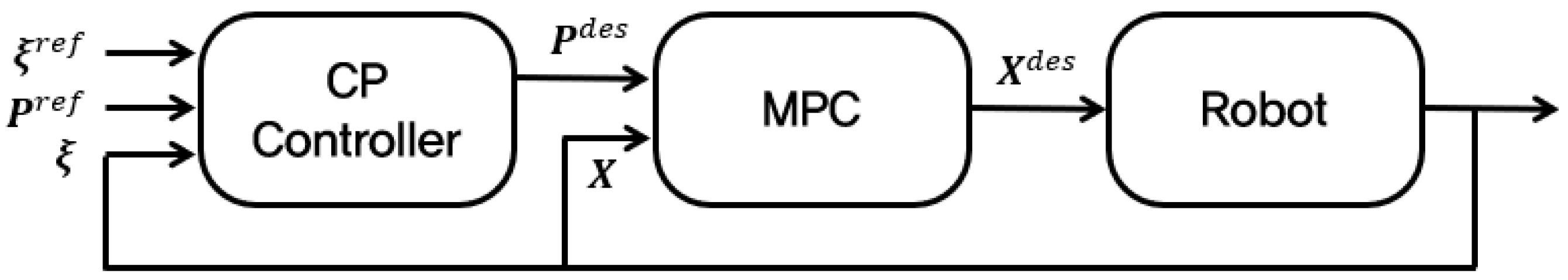
3.2. COM Trajectory Generation Using MPC

In this paper, linear MPC was used to generate COM trajectory for tracking the modified ZMP. Assuming that the jerk is constant over the interval $0 \le t < T$ and given the control step time T, the state at any discrete time step $k + 1$ can be expressed:

$$\begin{array}{cc}\hfill {\mathit{x}}_{k+1}& \hfill ={\mathit{Ax}}_k+\mathit{B}{\stackrel{⃛}{x}}_k\hfill \end{array}$$

(16)

where

$$\begin{array}{c}\hfill {\mathit{x}}_k=\left[\begin{array}{c}{x}_k\\ {\dot{x}}_k\\ {\ddot{x}}_k\end{array}\right],\mathit{A}=\left[\begin{array}{ccc}1& T& T^2/2\\ 0& 1& T\\ 0& 0& 1\end{array}\right],\mathit{B}=\left[\begin{array}{c}{T}^3/6\\ T^2/2\\ T\end{array}\right]\end{array}$$

Equation (2a) with discrete time can be expressed:

$$\begin{array}{c}\hfill {\mathit{P}}_k=x_k-{\displaystyle \frac{1}{{\omega }^2}}{\ddot{x}}_k=\left[\begin{array}{ccc}1& 0& -1/{\omega }^2\end{array}\right]{\mathit{x}}_k=\mathit{C}{\mathit{x}}_k\end{array}$$

(17)

With a prediction horizon of n steps,

$$\begin{array}{cc}\hfill {\mathit{X}}_{k+1}& \hfill =\hat{\mathit{A}}{\mathit{x}}_k+\hat{\mathit{B}}{\stackrel{⃛}{\mathit{X}}}_k\hfill \end{array}$$

(18)

$$\begin{array}{cc}\hfill {\mathit{P}}_{k+1}& \hfill ={\mathit{P}}_{ps}{\mathit{x}}_k+{\mathit{P}}_{pu}{\stackrel{⃛}{\mathit{X}}}_k\hfill \end{array}$$

(19)

where

$$\begin{array}{c}{\mathit{X}}_{k+1}=\left[\begin{array}{c}{\mathit{x}}_{k+1}\\ {\mathit{x}}_{k+2}\\ ⋮\\ {\mathit{x}}_{k+n}\end{array}\right],\widehat{\mathit{A}}=\left[\begin{array}{c}\mathit{A}\\ {\mathit{A}}^2\\ ⋮\\ {\mathit{A}}^n\end{array}\right],\widehat{\mathit{B}}=\left[\begin{array}{cccc}\mathit{B}& \mathit{0}& \dots & \mathit{0}\\ \mathit{AB}& \mathit{B}& \dots & \mathit{0}\\ ⋮& ⋮& \ddots & ⋮\\ {\mathit{A}}^{n-1}\mathit{B}& {\mathit{A}}^{n-2}\mathit{B}& \dots & \mathit{B}\end{array}\right],{\stackrel{⃛}{\mathit{X}}}_k=\left[\begin{array}{c}{\stackrel{⃛}{x}}_k\\ {\stackrel{⃛}{x}}_{k+1}\\ ⋮\\ {\stackrel{⃛}{x}}_{k+n-1}\end{array}\right]\\ {\mathit{P}}_{k+1}=\left[\begin{array}{c}{P}_{k+1}\\ P_{k+2}\\ ⋮\\ P_{k+n}\end{array}\right],{\mathit{P}}_{ps}=\left[\begin{array}{c}\mathit{CA}\\ {\mathit{CA}}^2\\ ⋮\\ {\mathit{CA}}^n\end{array}\right],{\mathit{P}}_{pu}=\left[\begin{array}{cccc}\mathit{CB}& \mathit{0}& \dots & \mathit{0}\\ \mathit{CAB}& \mathit{CB}& \dots & \mathit{0}\\ ⋮& ⋮& \ddots & ⋮\\ \mathit{C}{\mathit{A}}^{n-1}\mathit{B}& \mathit{C}{\mathit{A}}^{n-2}\mathit{B}& \dots & \mathit{CB}\end{array}\right]\end{array}$$

At any time instance, the velocity state can be expressed:

$$\begin{array}{c}\hfill {\dot{\mathit{X}}}_{k+1}={\mathit{P}}_{vs}{\mathit{x}}_k+{\mathit{P}}_{vu}{\stackrel{⃛}{\mathit{X}}}_k\end{array}$$

(20)

where

$$\begin{array}{c}\hfill {\mathit{P}}_{vs}=\left[\begin{array}{ccc}0& 1& T\\ 0& 1& 2T\\ ⋮& ⋮& ⋮\\ 0& 1& nT\end{array}\right],{\mathit{P}}_{vu}=\left[\begin{array}{cccc}{T}^2/2& 1& \dots & T\\ T^2/2+T^2& T^2/2& \dots & 2T\\ ⋮& ⋮& \ddots & ⋮\\ T^2/2+(n-1)T^2& T^2+(n-2)T^2& \dots & T^2/2\end{array}\right]\end{array}$$

The objective function was designed to achieve ZMP tracking and generate stable COM motions. The objective function is formulated as:

$$\begin{array}{c}\hfill \underset{{\mathit{P}}_{k+1}}{min}{\displaystyle \frac{\alpha }{2}}{\left|{\stackrel{⃛}{\mathit{X}}}_k\right|}^2+{\displaystyle \frac{\beta }{2}}{\left|{\dot{\mathit{X}}}_{k+1}\right|}^2+{\displaystyle \frac{\gamma }{2}}{\left|{\mathit{P}}_{k+1}-{\mathit{P}}_{k+1}^{des}\right|}^2\end{array}$$

(21)

This can be expressed in a quadratic form as:

$$\begin{array}{c}\hfill \underset{{\mathit{P}}_{k+1}}{min}{\displaystyle \frac{1}{2}}{\mathit{P}}_{k+1}^T{\mathit{QP}}_{k+1}+{\mathit{f}}^T{\mathit{P}}_{k+1}\end{array}$$

(22)

where

$$\begin{array}{c}\mathit{Q}=\alpha {\mathit{P}}_{pu}^{-T}{\mathit{P}}_{pu}^{-1}+\beta {\mathit{P}}_{pu}^{-T}{\mathit{P}}_{vu}^T{\mathit{P}}_{vu}{\mathit{P}}_{pu}^{-1}+\gamma \mathit{E}\\ \mathit{f}=\left[\beta {\mathit{P}}_{pu}^{-T}{\mathit{P}}_{vu}^T\left({\mathit{P}}_{vs}-{\mathit{P}}_{vu}{\mathit{P}}_{pu}^{-1}{\mathit{P}}_{ps}\right)-\alpha {\mathit{P}}_{pu}^{-T}{\mathit{P}}_{pu}{\mathit{P}}_{ps}\right]{\mathit{x}}_k-\gamma {\mathit{P}}_{k+1}^{des}\end{array}$$

where $\alpha$ is the jerk gain, $\beta$ is the velocity gain, and $\gamma$ is the ZMP tracking gain. $\mathit{E}\in {\mathbb{R}}^{n\times n}$ is the identity matrix.

The objective function in Equation (21) is designed to achieve several critical goals for stable and smooth locomotion. Specifically, the term penalizing jerk promotes smoother COM trajectories by minimizing rapid changes in acceleration. The velocity term helps to prevent excessively fast COM movements that could lead to instability or violate physical limits. The ZMP tracking term is crucial for maintaining the balance of the robot by ensuring the ZMP follows its desired reference. The Shceme of the MPC is shown in Figure 4.

The velocity trajectory of the COM was obtained with optimized ${\mathit{P}}_{k+1}$ based on Equations (19) and (20):

$$\begin{array}{c}\hfill {\dot{\mathit{X}}}_{k+1}={\mathit{P}}_{vs}{\mathit{x}}_k+{\mathit{P}}_{vu}{\mathit{P}}_{pu}^{-1}\left({\mathit{P}}_{k+1}-{\mathit{P}}_{ps}{\mathit{x}}_k\right)\end{array}$$

(23)

With the designed CP controller and MPC, the trajectory of the COM is generated only for the x and y axes. A separate MPC was used to generate the trajectory of the COM height. In Equation (21), the component for ZMP tracking was replaced with a component that keeps the height fixed, and an objective function was formulated using jerk as the control input.

$$\begin{array}{c}\hfill \underset{{\stackrel{⃛}{\mathit{Z}}}_k}{min}{\displaystyle \frac{{\alpha }_z}{2}}{\left|{\stackrel{⃛}{\mathit{Z}}}_k\right|}^2+{\displaystyle \frac{{\beta }_z}{2}}{\left|{\dot{\mathit{Z}}}_{k+1}\right|}^2+{\displaystyle \frac{{\gamma }_z}{2}}{\left|{\mathit{Z}}_{k+1}-{\mathit{Z}}_{k+1}^{des}\right|}^2=\underset{{\stackrel{⃛}{\mathit{Z}}}_k}{min}{\displaystyle \frac{1}{2}}{\stackrel{⃛}{\mathit{Z}}}_k^T{\mathit{Q}}_z{\stackrel{⃛}{\mathit{Z}}}_k+{\mathit{f}}_z^T{\stackrel{⃛}{\mathit{Z}}}_k\end{array}$$

(24)

where

$$\begin{array}{c}{\mathit{Q}}_z={\alpha }_z\mathit{E}+{\beta }_z{\mathit{P}}_{vu}^T{\mathit{P}}_{vu}+{\gamma }_z{\widehat{\mathit{B}}}^T\widehat{\mathit{B}}\\ {\mathit{f}}_z={\beta }_z{\mathit{P}}_{vu}^T{\mathit{P}}_{vs}{\mathit{z}}_k+{\gamma }_z{\widehat{\mathit{B}}}^T\left(\widehat{\mathit{A}}{\mathit{z}}_k-{\mathit{Z}}_{k+1}^{des}\right)\end{array}$$

where ${\alpha }_z$ is the jerk gain, ${\beta }_z$ is the velocity gain, and ${\gamma }_z$ is the height tracking gain.

Velocity trajectory of the COM in the vertical direction was obtained with optimized ${\stackrel{⃛}{\mathit{Z}}}_k$:

$$\begin{array}{c}\hfill {\dot{\mathit{Z}}}_{k+1}={\mathit{P}}_{vs}{\mathit{z}}_k+{\mathit{P}}_{vu}{\stackrel{⃛}{\mathit{Z}}}_k\end{array}$$

(25)

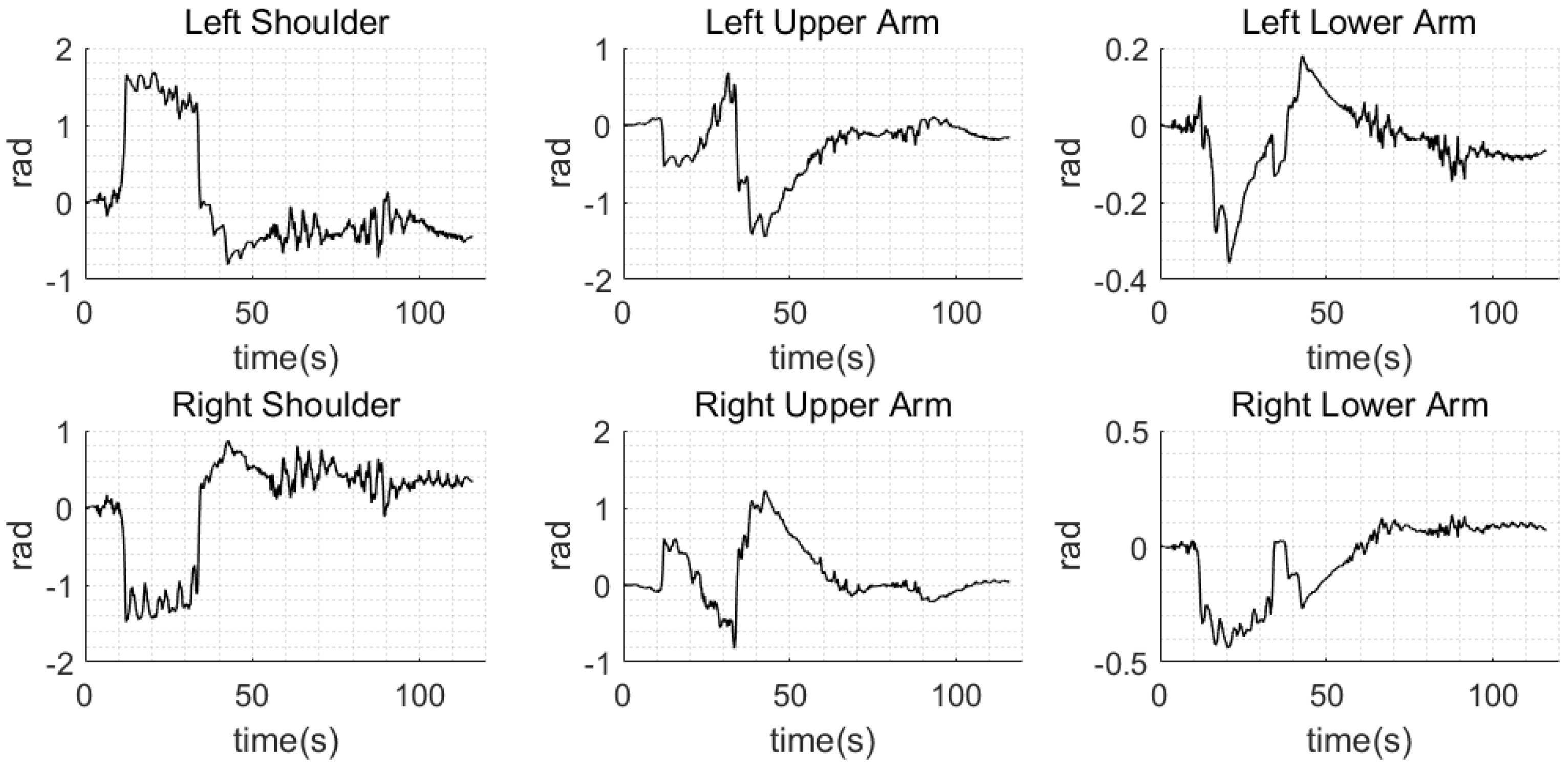
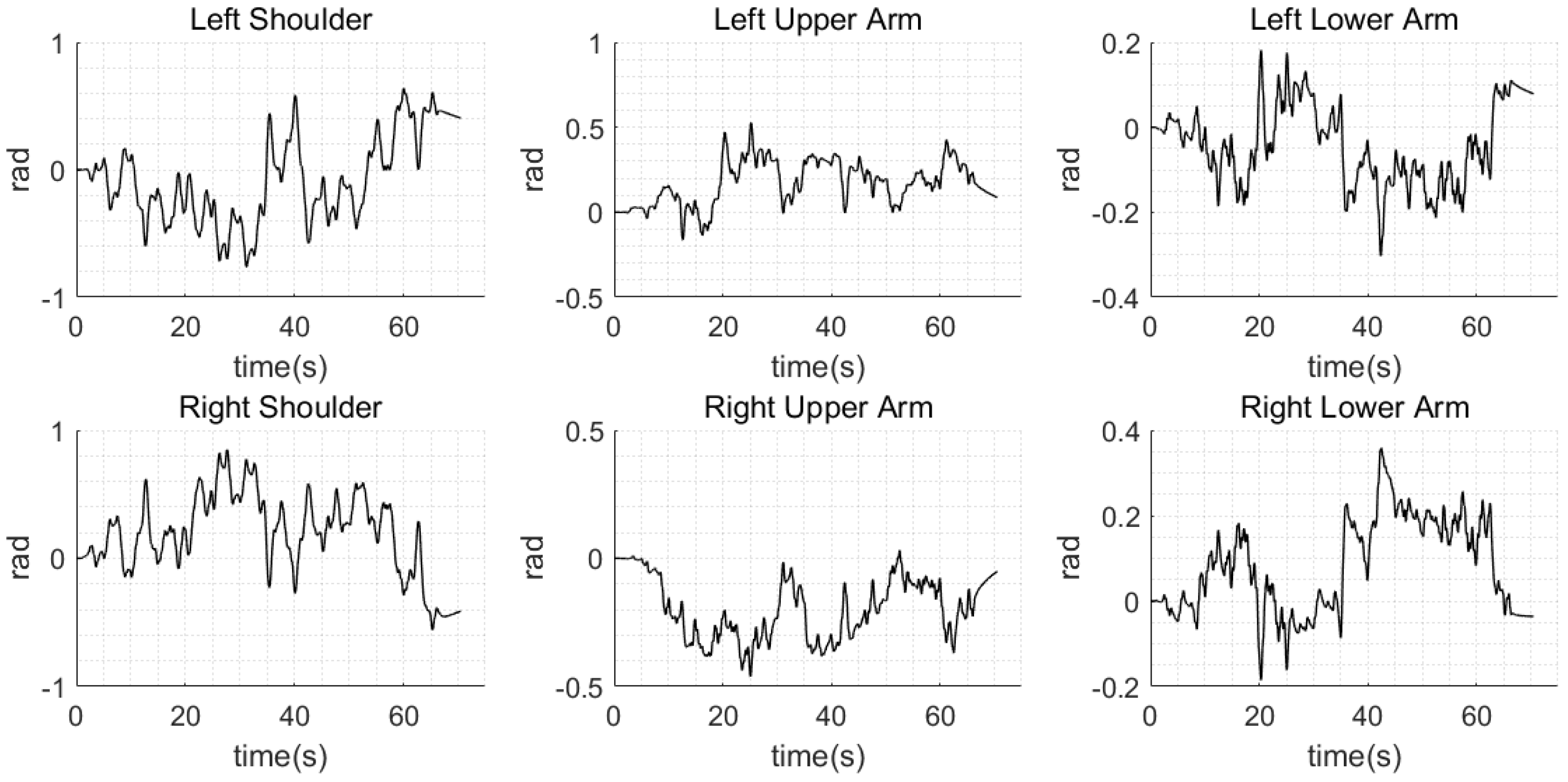
4. Generation of Arm Motion

The LIPM used to describe the robot is represented as a point mass, which inevitably leads to significant differences from the actual robot behavior. In particular, LIPM cannot represent angular momentum, which is closely related to the balance of the robot. This paper proposes a method for minimizing the angular momentum by generating arm motion based on the momentum equation and optimization. Balancing can be improved during various motions by minimizing angular momentum.

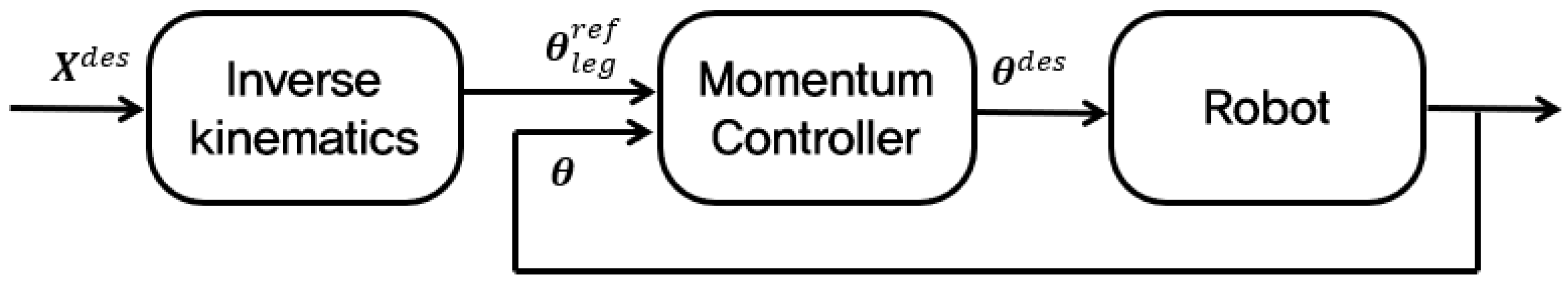
4.1. Momentum Equation

The angular momentum equation of the robot can be derived in a simplified form using all joint velocities, $\dot{\mathsf{\theta }}$ [24]. All angular momentum values in this paper are expressed with respect to the COM.

$$\begin{array}{c}\hfill \mathit{H}={\mathit{I}}_r{\mathsf{\omega }}_B+{\mathit{H}}_{\dot{\theta }}\dot{\mathsf{\theta }}\end{array}$$

(26)

where ${\mathit{I}}_r$ is the $3 \times 3$ inertia matrix with respect to the COM, and ${\mathsf{\omega }}_B$ is the angular velocity of the base link. ${\mathit{H}}_{\dot{\theta }}$ is the $3 \times m$ inertia matrix that indicates how the joint velocities affect the angular momentum. m is the number of joints.

Since ${\mathit{H}}_{\dot{\theta }}\dot{\mathsf{\theta }}$ is linear, Equation (26) can be decomposed into the leg and arm joint components.

$$\begin{array}{c}\hfill \mathit{H}={\mathit{I}}_r{\mathsf{\omega }}_B+\sum _{i=1}^2{\mathit{H}}_{leg,i}{\dot{\mathsf{\theta }}}_{leg,i}+{\mathit{H}}_{arm}{\dot{\mathsf{\theta }}}_{arm}\end{array}$$

(27)

where $H_{arm}$ and $H_{leg,i}$ denote the $3 \times 6$ inertia matrices that indicate how the arm and the leg joint velocities affect the angular momentum, respectively.

4.2. Momentum Control Using Optimization

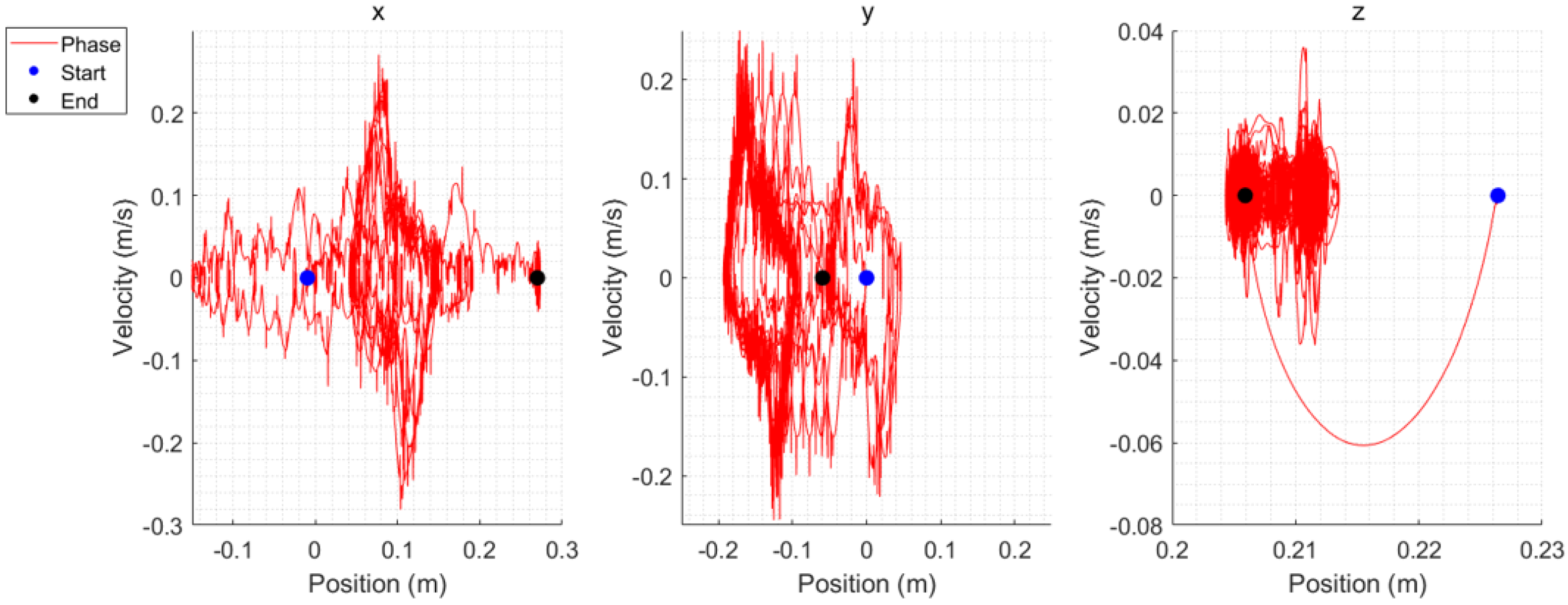
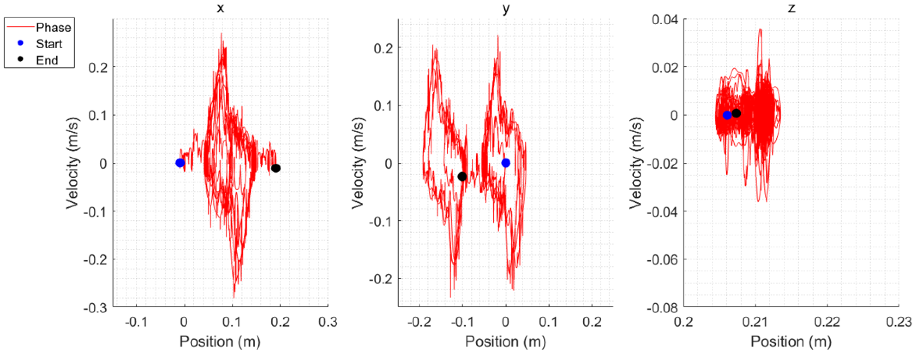
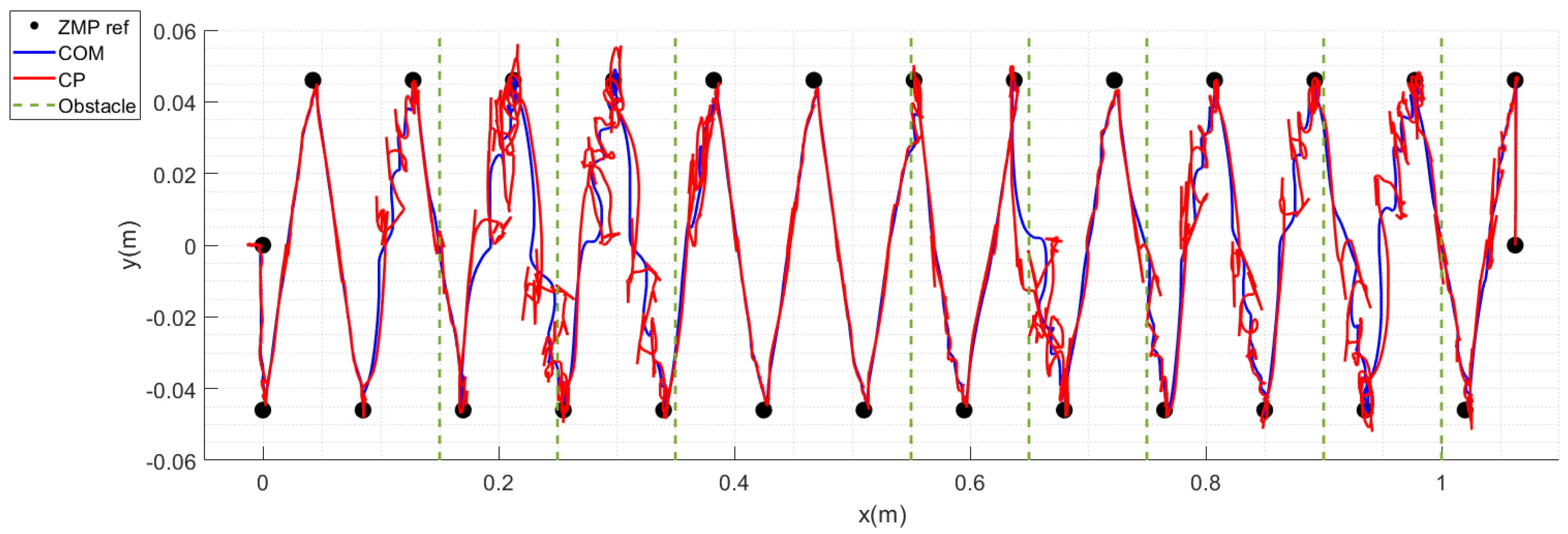
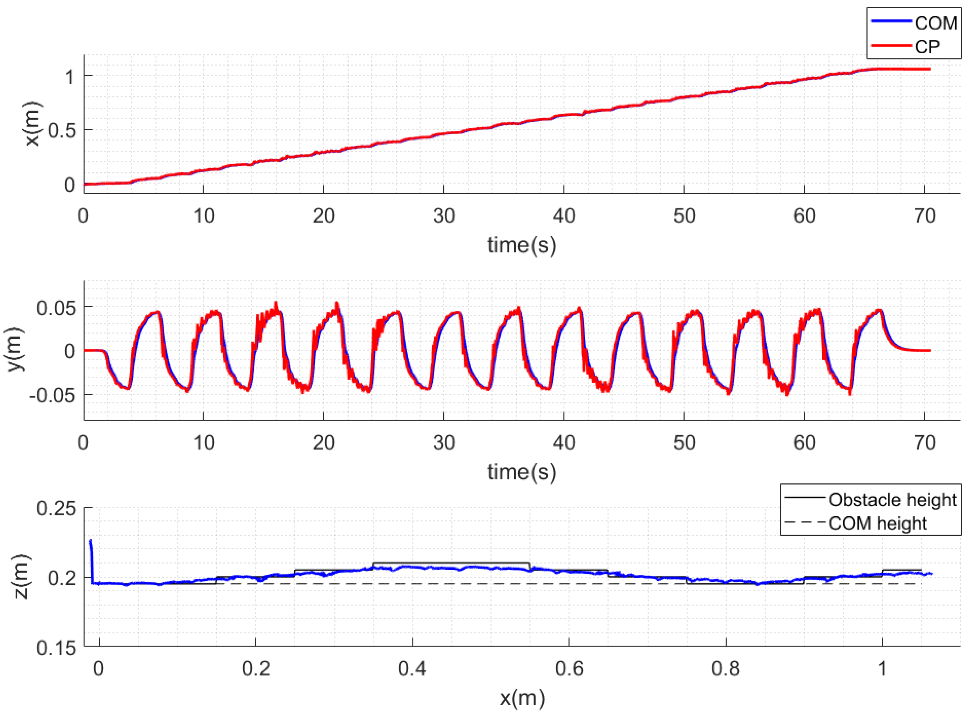
Using the momentum equation and optimization, the arm motion that minimizes the angular momentum of a biped robot can be obtained. Since forward kinematics allow the calculation of joint angles and position information, MPC could be applied over multiple steps, as with COM. However, due to the high computational cost, optimization was applied only to a single step.

With control step time $T_s$, the arm joint angle state ${\mathsf{\theta }}_{arm,k}$ at time instance $k+1$ is represented by control input ${\mathit{u}}_k$, which corresponds to the angular acceleration of the arm joint ${\ddot{\mathsf{\theta }}}_{arm,k}$:

$$\begin{array}{c}{\mathsf{\theta }}_{arm,k+1}={\mathsf{\theta }}_{arm,k}+T_s{\dot{\theta }}_{arm,k}+{\displaystyle \frac{T_s^2}{2}}{\mathit{u}}_k\end{array}$$

(28)

$$\begin{array}{c}{\dot{\mathsf{\theta }}}_{arm,k+1}={\dot{\mathsf{\theta }}}_{arm,k}+T_s{\mathit{u}}_k\end{array}$$

(29)

From Equation (27),

$$\begin{array}{c}\hfill {\mathit{H}}_k={\mathit{H}}_{arm,k}{\dot{\mathsf{\theta }}}_{arm,k}+{\mathit{D}}_k\end{array}$$

(30)

where $D_k$ represents the angular momentum contribution from the base and the legs at time instance k:

$$\begin{array}{c}{\mathit{D}}_k={\left|{\mathit{I}}_r{\mathsf{\omega }}_B+\sum _{i=1}^2{\mathit{H}}_{leg,i}{\dot{\mathsf{\theta }}}_{leg,i}\right|}_k\end{array}$$

Large movements of the arm can negatively affect balance, so the objective function was designed to generate minimal arm motions that reduce the angular momentum. Since the angular momentum varies across different axes, a selection matrix $\mathit{S}$ was introduced to prevent any single axis from becoming dominant. Additionally, by adjusting the elements of this selection matrix, it is possible to choose which axes to control. The objective function with selection matrix be:

$$\begin{array}{c}\underset{{\mathit{u}}_k}{min}{\displaystyle \frac{{\alpha }_A}{2}}{\left|{\mathit{u}}_k\right|}^2+{\displaystyle \frac{{\beta }_A}{2}}{\left|{\dot{\mathsf{\theta }}}_{k+1}\right|}^2+{\displaystyle \frac{{\gamma }_A}{2}}{\left|\mathit{S}{\mathit{H}}_{k+1}-\mathit{S}{\mathit{H}}_{k+1}^{ref}\right|}^2+{\displaystyle \frac{{\delta }_A}{2}}{\left|{\mathsf{\theta }}_{k+1}-{\mathsf{\theta }}_{k+1}^{ref}\right|}^2\\ =\underset{{\mathit{u}}_k}{min}{\displaystyle \frac{1}{2}}{\mathit{u}}_k^T{\mathit{Q}}_A{\mathit{u}}_k+{\mathit{f}}_A^T{\mathit{u}}_k\end{array}$$

(31)

where

$$\begin{array}{c}{\mathit{Q}}_A={\alpha }_A{\mathit{E}}_{+}{\beta }_A{T}_s^2+{\gamma }_A{T}_s^2{\left(\mathit{S}{\mathit{H}}_{arm,k+1}\right)}^T\left(\mathit{S}{\mathit{H}}_{arm,k+1}\right)+{\delta }_A{\displaystyle \frac{T_s^4}{4}}\\ {\mathit{f}}_A={\beta }_A{T}_s{\dot{\mathsf{\theta }}}_{arm,k}+{\gamma }_A{T}_s{\left(\mathit{S}{\mathit{H}}_{arm,k+1}\right)}^T\left(\mathit{S}{\mathit{H}}_{arm,k+1}{\dot{\mathsf{\theta }}}_k+\mathit{S}{\mathit{D}}_{k+1}-\mathit{S}{\mathit{H}}_{k+1}^{ref}\right)\\ +{\delta }_A{\displaystyle \frac{T_s^2}{2}}\left[\left({\mathsf{\theta }}_k-{\mathsf{\theta }}_{k+1}^{ref}\right)+T_s{\dot{\mathsf{\theta }}}_k\right]\\ \mathit{S}=\left[\begin{array}{ccc}{\alpha }_R& 0& 0\\ 0& {\alpha }_P& 0\\ 0& 0& {\alpha }_Y\end{array}\right]\end{array}$$

where ${\alpha }_A$ is the acceleration gain, ${\beta }_A$ is the velocity gain, ${\gamma }_A$ is the momentum gain, and ${\delta }_A$ is the angle gain. The value $0 \le {\alpha }_R, {\alpha }_P, {\alpha }_Y \le 1$ represent the roll, pitch, and yaw gains, respectively, and are used to adjust their influence.

The objective function in Equation (31) is designed to generate arm motions that actively contribute to the balance of the robot while ensuring the movements are smooth and natural. Minimizing joint acceleration encourages fluid changes in arm velocity and reduces control effort. Penalizing excessive joint velocity helps prevent overly fast or jerky arm movements that could otherwise destabilize the robot. The core of the objective function is the angular momentum tracking term, which drives the arms to generate compensatory momentum, thereby stabilizing the overall robot posture. Including an angle error term helps to keep the arm joints near a reference configuration, preventing them from undesirable postures. Scheme of momentum controller is shown in Figure 5.

To reduce computation time, the inertia matrices ${\mathit{H}}_{arm,k+1}, {\mathit{H}}_{leg,k+1}, {\mathit{I}}_{r,k+1}$ used in $H_{k+1}$ and $D_{k+1}$ were assumed to be the same as those at step k. The time interval between step k and $k + 1$ is very short, so it was assumed that there are no meaningful changes in physical quantities.

5. Simulation

5.1. Simulation Environment

The proposed methods were validated through simulations. We constructed a simulator with Robotis DARwin-OP. Each arm has three degrees of freedom, and each leg has six degrees of freedom. Including the two degrees of freedom in the neck, the robot has a total of 20 degrees of freedom, but only 18 were used by controlling only the arms and legs. The size and appearance of the DARwin-OP used in the simulation are shown in Figure 6. The weight of each part is shown in

Table 1. Weight of each part.

Part	Mass (kg)
Body	$0.976$
Head	$0.158$
Neck	$0.024$
Shoulder (2)	$0.013$
Upper arm (2)	$0.168$
Lower arm (2)	$0.016$
Pelvic (2)	$0.194$
Thigh (2)	$0.119$
Tibia (2)	$0.070$
Ankle (2)	$0.167$
Foot (2)	$0.079$
Total	$2.925$

.

The overall structure of the proposed methods implemented in the simulation is shown in Figure 7. The validation was conducted in different environments, including flat ground with direction changes, varying step length and walking cycles, and an environment with stair-like obstacles that were not recognized in advance. The simulator was built using RecurDyn (V8R5) and Simulink (Version 10.2), running on a system with a 64-bit AMD Ryzen 7 1700 CPU at 3 GHz (Advanced Micro Devices, Inc., Santa Clara, CA, USA). For simulations, RecurDyn was used with Simulink, where RecurDyn provided the platform for multi-body dynamics simulation, and Simulink was used for control system simulation. As a multi-body dynamics analysis software, the solver of RecurDyn is based on equations of motion derived from a recursive formulation, which facilitates fast and high-precision analysis [33]. Furthermore, RecurDyn provides a variety of contact and joint modeling options, enabling a detailed analysis of complex systems [34]. All algorithms were implemented in MATLAB (The MathWorks, Inc., Natick, MA, USA). The optimization problems were solved using the quadprog function provided in MATLAB (R2020b).

In all simulations, the prediction horizon n is set to 10, and the sampling time $T_s$ is set to 2 ms. During the simulation, the gain values of the selection matrix were determined based on the angular momentum value of each axis. The gains used for all controllers are shown in

Table 2. The gains used for all controllers.

Gain	Value
$k_{cp,x}, k_{cp,y}$	$-700$
${\alpha }_x, {\alpha }_y$	30
${\beta }_x, {\beta }_y$	$5 \times {10}^5$
${\gamma }_z, {\gamma }_y$	$1 \times {10}^{10}$
${\alpha }_z$	$5.0$
${\beta }_z$	$1 \times {10}^6$
${\gamma }_z$	$1 \times {10}^9$
${\alpha }_A$	$1 \times {10}^4$
${\beta }_A$	600
${\gamma }_A$	$7 \times {10}^8$
${\delta }_A$	$7 \times {10}^{10}$
${\alpha }_R$	$0.20$
${\alpha }_P$	$0.25$
${\alpha }_Y$	$1.0$

. With the exception of those for the selection matrix, the controller gains were determined through an empirical tuning process. The gains used in the selection matrix were adjusted by considering the values of the angular momentum observed in the simulation results. While a formal sensitivity analysis was not conducted as part of this study, the gains were carefully selected through iterative individual adjustments and observation of the resulting system performance to ensure robust operation.

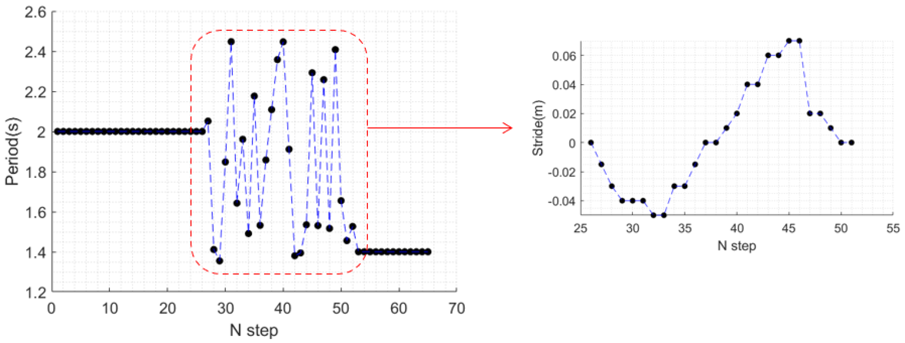
5.2. Variable Stride and Step Period

To verify the stability of motion under various movements, simulations of rotational, forward, backward, and lateral movements were conducted on flat ground. A total of 63 steps were performed. Rotational motions were from step 5 to step 25 with a step period of 2 s, alternating counter-clockwise and clockwise by $\pi /2$. During forward and backward motion from step 26 to step 51, the step period and stride were randomly varied. From step 52 to step 63, lateral motion was performed with a step period of $1.4$ s and a stride of 16 mm. Changes in gait are shown in Figure 8.

The overall simulation results are shown in Figure 9. The robot maintained stability without falling in all motions. The predefined footstep reference ZMP, along with the COM and the CP, are represented in Figure 10 by black circles, blue lines, and red lines, respectively. The COM and CP for each axis are shown in Figure 11.

The arm motion generated by the momentum controller is shown in Figure 12. The angular momentum of the COM and the linear velocity of the robot are presented in Figure 13. The red line represents locomotion without arm usage, while the blue line represents locomotion with arm motion. The overall amplitude of angular momentum and the linear velocity decreased in the blue line, demonstrating that utilizing arm motion contributes to more stable walking. The sum of the absolute angular momentum values decreased by $0.134\%$, $1.18\%$, and $21.2\%$ for the $x, y$, and z axes, respectively. The peak magnitudes decreased by $13.2\%$, $18.8\%$, and $12.0\%$, respectively.

Figure 14 and Figure 15 present the phase plots of the COM position and velocity for all steps and during rotational motion, respectively. Despite random variations in stride length and step period, the COM trajectories converge to stable limit cycles for each gait sequence, as shown in Figure 14, demonstrating the controller’s ability to maintain stability under changing locomotion parameters. The system robustly transitions between different attractors corresponding to each gait condition until it eventually settles at a stable fixed point upon stopping. Similarly, Figure 15 shows that during both counterclockwise and clockwise rotations, the phase plots exhibit consistent and bounded patterns, indicating that the proposed control framework successfully stabilizes the motion of the robot even during complex turning maneuvers. These results empirically support the stability of the integrated control system when subjected to varying gait demands.

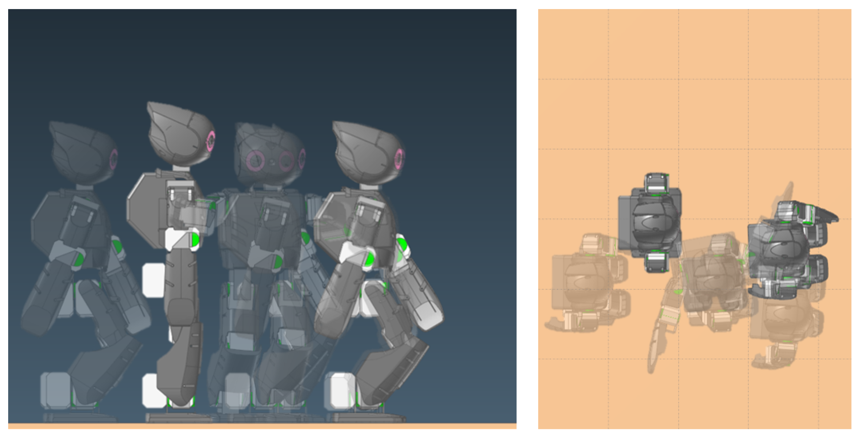
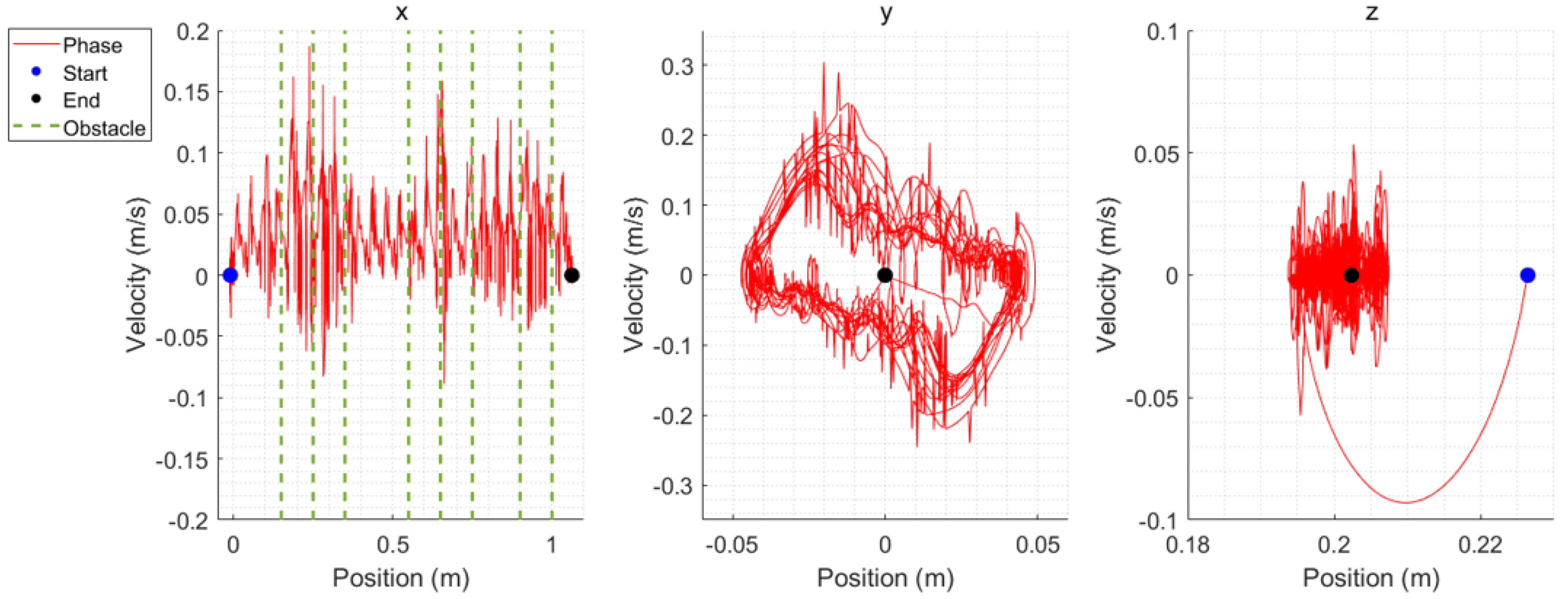
5.3. Unexpected Obstacles

To evaluate whether stable walking is achieved even in environments with unexpected obstacles, a simulation was implemented in an environment with stair-shaped obstacles. The step period was fixed at $2.5$ s and the stride at 85 mm. The robot was unaware of any obstacles in advance. The placement and height of the obstacles, relative to the starting position at the origin, are shown in

Table 3. Obstacle location and height.

Location (mm)	Height (mm)
150∼250	5
250∼350	10
350∼550	15
550∼650	10
650∼750	5
900∼1000	5
1000∼1200	10

.

The overall simulation results are shown in Figure 16. Stable motion was achieved without falling in the presence of unexpected obstacles. The predefined footstep reference ZMP, along with the COM trajectory and CP, are represented in Figure 17 by black circles, blue lines, and red lines, respectively. The COM and CP for each axis are shown in Figure 18.

The arm motion generated by the momentum controller is shown in Figure 19. The angular momentum of the COM and the linear velocity of the robot are presented in Figure 20. The red line represents locomotion without arm usage, while the blue line represents locomotion with arm motion. Without a momentum controller, the robot lost balance and fell when stepping on obstacles. This difference was attributed to the increased inertia tensor of the robot due to arm posture changes, as shown in Figure 21, which made the robot less affected by external forces.

The stability of the robot when encountering unexpected obstacles is shown by the phase plots in Figure 22 and Figure 23. Figure 22, showing the phase plot for all steps in the obstacle environment, demonstrates that the COM motion converges to and maintains a consistent, bounded trajectory, indicative of overall system stability. More specifically, Figure 23 details the phase plot as the robot steps over obstacles. While transient deviations are observed in the trajectories due to the impulsive forces from the obstacles, the system recovers, and the COM state converges back to a stable, periodic pattern. This recovery and convergence to a consistent pattern, even after unpredicted disturbances, indicate the robustness and stabilizing capability of the proposed whole-body motion generation framework.

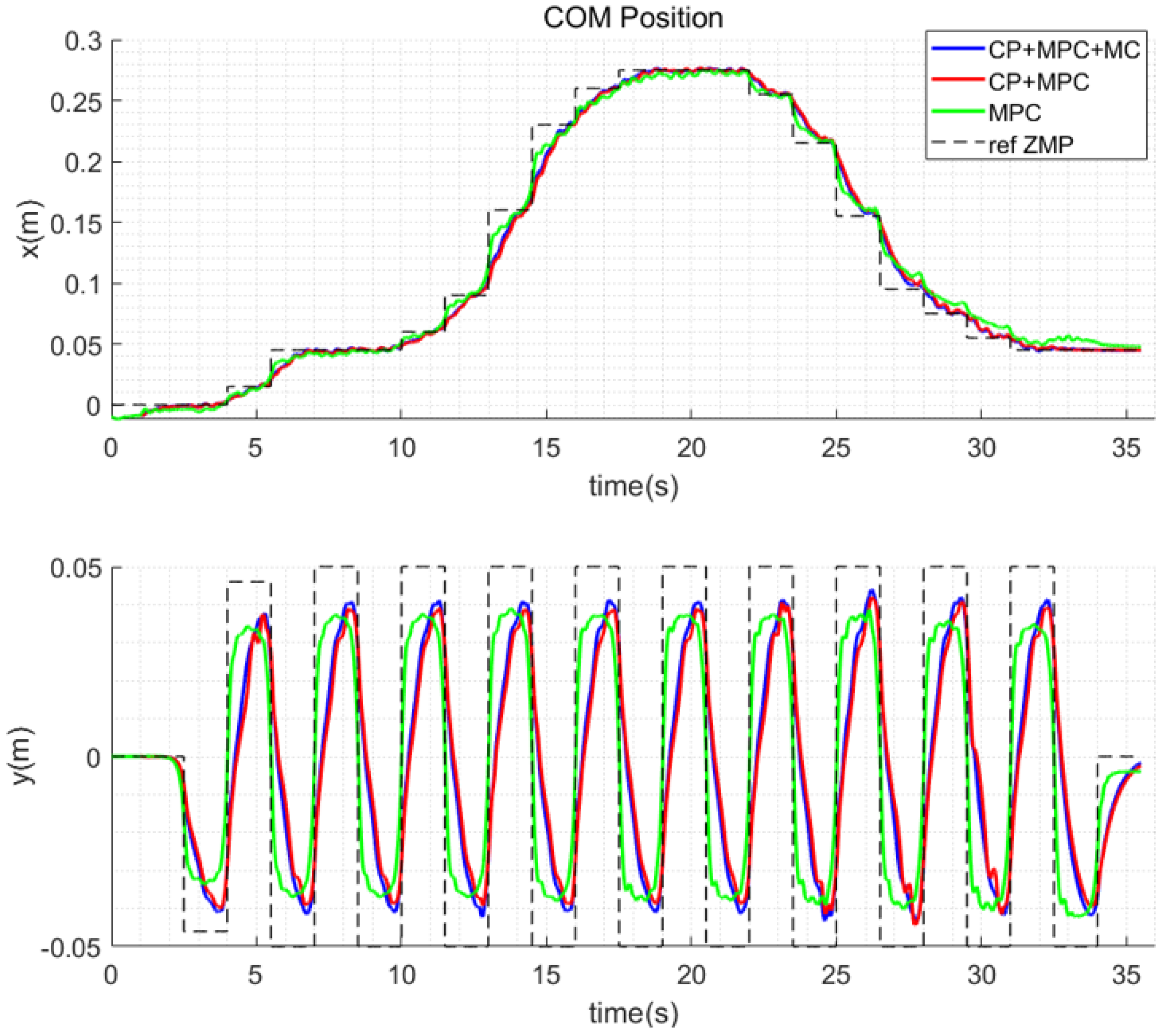
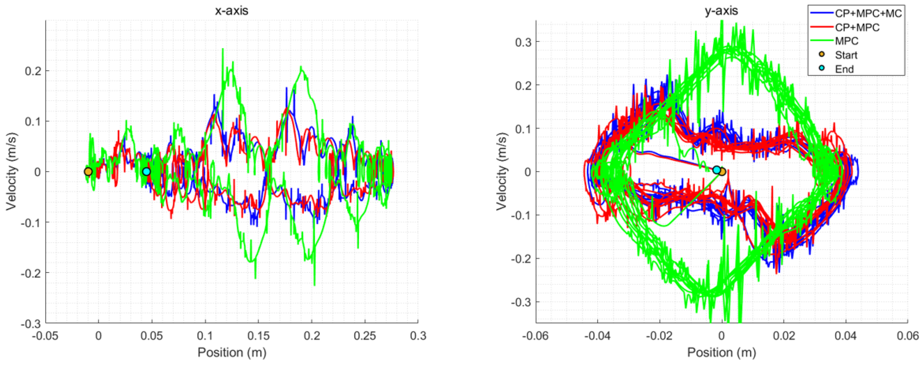
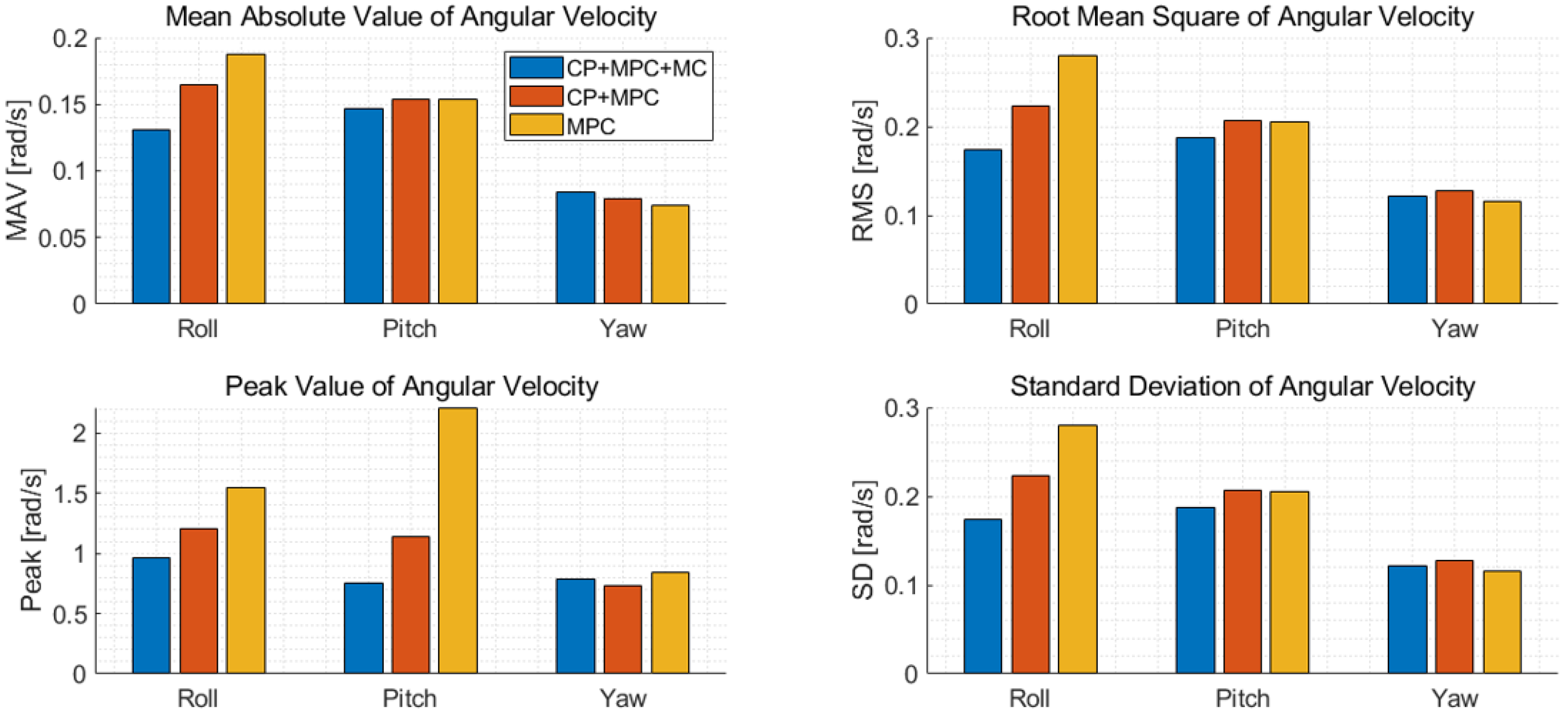
5.4. Comparative Analysis

To quantitatively evaluate the performance of the proposed whole-body motion generation framework, a comparative analysis was conducted against two baseline controllers: a simple ZMP tracking controller based on MPC and an MPC combined with CP control (CP+MPC). The proposed framework is denoted as CP+MPC+MC. All controllers were tasked with generating simple walking motions under identical conditions. The following analyses focus on ZMP tracking accuracy and angular momentum and velocity of robot body characteristics.

Figure 24 illustrates the COM trajectories in the x and y directions for each controller, alongside the reference ZMP, dashed black line. While the controllers generally follow the desired path, CP+MPC-based frameworks (blue and red lines) exhibit smoother COM motion with less deviation from the reference ZMP steps, particularly in the y-axis, compared to MPC alone.

The ZMP tracking performance is further detailed in Figure 25. Across all metrics—mean absolute value (MAV), root mean square (RMS), peak value, and standard deviation (SD)—the CP+MPC-based controllers consistently demonstrate lower ZMP tracking errors in both x and y axes. Notably, the inclusion of CP control significantly reduces the errors compared to the MPC-only approach. This indicates enhanced stability and precision in ZMP tracking with the CP control framework.

The stability of the generated gaits is also visualized through phase plots of COM position versus velocity, as shown in Figure 26. Frameworks incorporating the CP controller (CP+MPC and CP+MPC+MC) result in compact and consistent limit cycles for both x and y axes, suggesting a more stable gait pattern compared to the wider and more dispersed trajectories produced by MPC alone.

Figure 27 presents a comparison of the whole-body angular momentum. The CP+MPC framework already shows a reduction in angular momentum compared to MPC alone, indicating improved inherent stability. The introduction of the momentum controller leads to a further notable decrease in angular momentum across all axes and metrics, particularly in the roll and pitch directions. This highlights the effectiveness of the arm motion in actively minimizing overall body angular momentum.

The impact on the angular velocity of the body is shown in Figure 28. A significant reduction in angular velocity, especially in the roll and pitch axes, is observed for the CP+MPC+MC. While the angular momentum itself might show moderate reductions with momentum controller compared to CP+MPC in some instances, the substantial decrease in angular velocity suggests an increase in the inertia tensor of the robot, as depicted in Figure 29. The arm motions effectively increase the moment of inertia. This increased inertia provides greater resistance to rotational disturbances, meaning that for a similar external disturbing torque, the robot experiences less angular acceleration, contributing to enhanced system stability.

Compared to the simple ZMP tracking controller based on MPC, the proposed whole-body framework (CP+MPC+MC) demonstrated a significant reduction in ZMP tracking errors. Specifically, the MAV of the ZMP tracking error decreased by approximately $23.9\%$ in the x-axis and $32.3\%$ in the y-axis. Similarly, the peak ZMP tracking error was reduced by about $42.9\%$ in the x-axis and $46.8\%$ in the y-axis. While the peak ZMP tracking error, which can appear larger due to the inclusion of acceleration components in ZMP calculation and thus may be less reliable as a sole indicator, nonetheless showed an overall decreasing trend.

Furthermore, when the momentum controller was utilized, CP+MPC+MC, a notable change in the angular velocity of the body was observed compared to using only CP+MPC. The MAV of angular velocity decreased by approximately $20.3\%$ in the roll and $4.9\%$ in the pitch, while the peak angular velocity decreased by about $19.9\%$ in the roll and $33.8\%$ in the pitch. Although the MAV and peak angular velocity in the yaw slightly increased by $5.9\%$ and $7.0\%$, respectively, the substantial improvements in the roll and pitch directions clearly indicate an enhancement in balancing performance due to the arm motion.

In summary, these comparative analyses demonstrate that the proposed whole-body motion framework (CP+MPC+MC) achieves more stable and precise locomotion. The CP control enhances ZMP tracking and COM stability. Meanwhile, the momentum controller, by generating active arm motion, not only further reduces angular momentum but also leverages the resulting larger inertia tensor to minimize angular velocity, thereby improving overall balance and robustness.

6. Conclusions

This paper proposed a method for generating stable whole-body motion for biped robots by integrating CP control, MPC for COM trajectory, and a momentum controller for arm motion. A decoupled momentum control approach was proposed to extend motion control for the upper body beyond conventional lower-body-centric control frameworks, improving balance during walking. Through simulations, the controllers were validated in various scenarios, including changes in stride and step period, as well as environments with unexpected obstacles. The simulation results demonstrate that the proposed method effectively stabilizes the robot’s motion by reducing angular momentum fluctuations and improving balance. By utilizing a momentum controller, the robot was able to counteract destabilizing forces, allowing it to walk more reliably even when stepping on unanticipated obstacles. Comparative results between cases with and without arm motion showed improvements in balance. The proposed whole-body motion framework is expected to contribute to the advancement of next-generation humanoid robots.

Despite these advancements, further improvements are needed to extend the applicability to more complex terrains. One potential enhancement is the force controller for the supporting foot. Future work will focus on implementing this force-based adaptation and expanding the framework to handle disturbance more effectively. Moreover, future research could delve into principles of embodied intelligence, potentially incorporating concepts, such as embodied adaptive motor neurons, to improve the robot’s interaction with complex environments.

References

1. Tong, Y.; Liu, H.; Zhang, Z. Advancements in humanoid robots: A comprehensive review and future prospects. IEEE/CAA J. Autom. Sin. 2024, 11, 301–328. [Google Scholar] [CrossRef]
2. Huang, H.; Liu, S.Q. Are consumers more attracted to restaurants featuring humanoid or non-humanoid service robots? Int. J. Hosp. Manag. 2022, 107, 103310. [Google Scholar] [CrossRef]
3. Song, C.S.; Kim, Y.K. The role of the human-robot interaction in consumers’ acceptance of humanoid retail service robots. J. Bus. Res. 2022, 146, 489–503. [Google Scholar] [CrossRef]
4. Darvish, K.; Penco, L.; Ramos, J.; Cisneros, R.; Pratt, J.; Yoshida, E.; Ivaldi, S.; Pucci, D. Teleoperation of humanoid robots: A survey. IEEE Trans. Robot. 2023, 39, 1706–1727. [Google Scholar] [CrossRef]
5. Vianello, L.; Penco, L.; Gomes, W.; You, Y.; Anzalone, S.M.; Maurice, P.; Thomas, V.; Ivaldi, S. Human-humanoid interaction and cooperation: A review. Curr. Robot. Rep. 2021, 2, 441–454. [Google Scholar] [CrossRef]
6. Kajita, S.; Kanehiro, F.; Kaneko, K.; Yokoi, K.; Hirukawa, H. The 3D linear inverted pendulum mode: A simple modeling for a biped walking pattern generation. In Proceedings of the IEEE/RSJ International Conference on Intelligent Robots and Systems, Maui, HI, USA, 29 October–3 November 2001. [Google Scholar]
7. Park, J.H.; Kim, K.D. Biped robot walking using gravity-compensated inverted pendulum mode and computed torque control. In Proceedings of the IEEE International Conference on Robotics and Automation, Leuven, Belgium, 20–20 May 1998. [Google Scholar]
8. Cho, J.; Park, J.H. Model predictive control of running biped robot. Appl. Sci. 2022, 12, 11183. [Google Scholar] [CrossRef]
9. Nakaura, S.; Sampei, M. Balance control analysis of humanoid robot based on ZMP feedback control. In Proceedings of the International Conference on Intelligent Robots and Systems, Lausanne, Switzerland, 30 September–4 October 2002. [Google Scholar]
10. Kajita, S.; Kanehiro, F.; Kaneko, K.; Fujiwara, K.; Harada, K.; Yokoi, K.; Hirukawa, H. Biped walking pattern generation by using preview control of zero-moment point. In Proceedings of the IEEE International Conference on Robotics and Automation, Taipei, Taiwan, 14–19 September 2003. [Google Scholar]
11. Katayama, S.; Murooka, M.; Tazaki, Y. Model predictive control of legged and humanoid robots: Models and algorithms. Adv. Robot. 2023, 37, 298–315. [Google Scholar] [CrossRef]
12. Wieber, P.B. Trajectory free linear model predictive control for stable walking in the presence of strong perturbations. In Proceedings of the IEEE-RAS International Conference on Humanoid Robots, Genoa, Italy, 4–6 December 2006. [Google Scholar]
13. Herdt, A.; Perrin, N.; Wieber, P.B. LMPC based online generation of more efficient walking motions. In Proceedings of the IEEE-RAS International Conference on Humanoid Robots, Osaka, Japan, 29 November–1 December 2012. [Google Scholar]
14. Pratt, J.; Carff, J.; Drakunov, S.; Goswami, A. Capture point: A step toward humanoid push recovery. In Proceedings of the IEEE–RAS International Conference on Humanoid Robots, Genoa, Italy, 4–6 December 2006. [Google Scholar]
15. Hof, A.L.; Gazendam, M.G.J.; Sinke, W.E. The condition for dynamic stability. J. Biomech. 2005, 38, 1–8. [Google Scholar] [CrossRef] [PubMed]
16. Takenaka, T.; Matsumoto, T.; Yoshiike, T. Real-time motion generation and control for biped robot—1st report: Walking gait pattern generation. In Proceedings of the IEEE/RSJ International Conference on Intelligent Robots and Systems, St. Louis, MO, USA, 10–15 October 2009. [Google Scholar]
17. Hof, A.L. The ‘extrapolated center of mass’ concept suggests a simple control of balance in walking. Hum. Mov. Sci. 2008, 27, 112–125. [Google Scholar] [CrossRef] [PubMed]
18. Englsberger, J.; Ott, C.; Roa, M.A.; Albu-Schäffer, A.; Hirzinger, G. Bipedal walking control based on capture point dynamics. In Proceedings of the IEEE/RSJ International Conference on Intelligent Robots and Systems, San Francisco, CA, USA, 25–30 September 2011. [Google Scholar]
19. Kamioka, T.; Kaneko, H.; Takenaka, T.; Yoshiike, T. Simultaneous optimization of ZMP and footsteps based on the analytical solution of divergent component of motion. In Proceedings of the IEEE International Conference on Robotics and Automation, Brisbane, QLD, Australia, 21–25 May 2018. [Google Scholar]
20. Herdt, A.; Diedam, H.; Wieber, P.B.; Dimitrov, D.; Mombaur, K.; Diehl, M. Online walking motion generation with automatic footstep placement. Adv. Robot. 2010, 24, 719–737. [Google Scholar] [CrossRef]
21. Shafiee-Ashtiani, M.; Yousefi-Koma, A.; Shariat-Panahi, M. Robust bipedal locomotion control based on model predictive control and divergent component of motion. In Proceedings of the IEEE International Conference on Robotics and Automation, Singapore, 29 May–3 June 2017. [Google Scholar]
22. Joe, H.M.; Oh, J.H. Balance recovery through model predictive control based on capture point dynamics for biped walking robot. Robot. Auton. Syst. 2018, 105, 1–10. [Google Scholar] [CrossRef]
23. Luo, X.; Xia, D.; Zhu, C. Planning and control of biped robots with upper body. In Proceedings of the IEEE/RSJ International Conference on Intelligent Robots and Systems, Daejeon, South Korea, 9–14 October 2016. [Google Scholar]
24. Kajita, S.; Kanehiro, F.; Kaneko, K.; Fujiwara, K.; Harada, K.; Yokoi, K.; Hirukawa, H. Resolved momentum control: Humanoid motion planning based on the linear and angular momentum. In Proceedings of the IEEE/RSJ International Conference on Intelligent Robots and Systems, Las Vegas, NV, USA, 27–31 October 2003. [Google Scholar]
25. Kajita, S.; Nagasaki, T.; Kaneko, K.; Hirukawa, H. ZMP-based biped running control. IEEE Robot. Autom. Mag. 2007, 14, 63–72. [Google Scholar] [CrossRef]
26. Lee, S.H.; Goswami, A. A momentum-based balance controller for humanoid robots on non-level and non-stationary ground. Auton. Robot. 2012, 33, 399–414. [Google Scholar] [CrossRef]
27. Otani, T.; Hashimoto, K.; Miyamae, S.; Ueta, H.; Sakaguchi, M.; Kawakami, Y.; Lim, H.O.; Takanishi, A. Angular momentum compensation in yaw direction using upper body based on human running. In Proceedings of the IEEE International Conference on Robotics and Automation, Singapore, 29 May–3 June 2017. [Google Scholar]
28. Kim, S.; Kim, C.; Park, J.H. Human-like arm motion generation for humanoid robots using motion capture database. In Proceedings of the 2006 IEEE/RSJ International Conference on Intelligent Robots and Systems, Beijing, China, 9–15 October 2006; pp. 3486–3491. [Google Scholar]
29. Yang, A.; Chen, Y.; Naeem, W.; Fei, M.; Chen, L. Humanoid motion planning of robotic arm based on human arm action feature and reinforcement learning. Mechatronics 2021, 78, 102630. [Google Scholar] [CrossRef]
30. Khazoom, C.; Kim, S. Humanoid arm motion planning for improved disturbance recovery using model hierarchy predictive control. In Proceedings of the 2022 International Conference on Robotics and Automation (ICRA), Philadelphia, PA, USA, 23–27 May 2022; pp. 6607–6613. [Google Scholar]
31. Englsberger, J.; Ott, C. Integration of vertical com motion and angular momentum in an extended capture point tracking controller for bipedal walking. In Proceedings of the IEEE-RAS International Conference on Humanoid Robots, Osaka, Japan, 29 November–1 December 2012. [Google Scholar]
32. Englsberger, J.; Ott, C.; Albu-Schäffer, A. Three-dimensional bipedal walking control using divergent component of motion. In Proceedings of the IEEE/RSJ International Conference on Intelligent Robots and Systems, Tokyo, Japan, 3–7 November 2013. [Google Scholar]
33. Kumar, S.; Rajeevlochana, C.G.; Saha, S.K. Realistic modeling and dynamic simulation of kuka kr5 robot using recurdyn. In Proceedings of the 6th Asian Conference on Multibody Dynamics, Shanghai, China, 26–30 August 2012. [Google Scholar]
34. Gummer, A.; Sauer, B. Modeling planar slider-crank mechanisms with clearance joints in RecurDyn. Multibody Syst. Dyn. 2014, 31, 127–145. [Google Scholar] [CrossRef]
Figure 1. Linear inverted pendulum model.
Applsci 15 05828 g001
Figure 2. Cascaded form between CP and COM dynamics.
Applsci 15 05828 g002
Figure 3. Scheme of CP control for stabilizing the divergent dynamics of the CP.
Applsci 15 05828 g003
Figure 4. Scheme of the MPC for COM trajectory generation to track the modified ZMP.
Applsci 15 05828 g004
Figure 5. Scheme of momentum control for generating arm motion.
Applsci 15 05828 g005
Figure 6. Robotic humanoid DARwin-OP.
Applsci 15 05828 g006
Figure 7. Overall flowchart.
Applsci 15 05828 g007
Figure 8. Changes in step period and stride.
Applsci 15 05828 g008
Figure 9. Overall progress of simulation.
Applsci 15 05828 g009
Figure 10. COM, CP position and reference ZMP.
Applsci 15 05828 g010
Figure 11. COM and CP of the robot.
Applsci 15 05828 g011
Figure 12. Generated arm motion.
Applsci 15 05828 g012
Figure 13. Angular momentum and linear velocity.
Applsci 15 05828 g013
Figure 14. Phase plot for all steps.
Applsci 15 05828 g014
Figure 15. Phase plot for rotational motion.
Applsci 15 05828 g015
Figure 16. Overall progress of simulation.
Applsci 15 05828 g016
Figure 17. COM, CP and reference ZMP.
Applsci 15 05828 g017
Figure 18. COM and CP of the robot.
Applsci 15 05828 g018
Figure 19. Generated arm motion.
Applsci 15 05828 g019
Figure 20. Angular momentum and linear velocity.
Applsci 15 05828 g020
Figure 21. Comparison of inertia tensor between arm usage.
Applsci 15 05828 g021
Figure 22. Phase plot for all steps.
Applsci 15 05828 g022
Figure 23. Phase plot during obstacle stepping.
Applsci 15 05828 g023
Figure 24. COM positions of each control framework.
Applsci 15 05828 g024
Figure 25. Comparison of ZMP tracking performance.
Applsci 15 05828 g025
Figure 26. Phase plot of each control framework.
Applsci 15 05828 g026
Figure 27. Comparison of angular momentum.
Applsci 15 05828 g027
Figure 28. Comparison of angular velocity.
Applsci 15 05828 g028
Figure 29. Inertia tensor of each control framework.
Applsci 15 05828 g029