Article

Prediction of Corroded Pipeline Failure Pressure Based on Empirical Knowledge and Machine Learning

1
School of Human Settlements and Civil Engineering, Xi′an Jiaotong University, Xi’an 710049, China
2
Shannxi Provincial Natural Gas Co., Ltd., Xi′an 710016, China
*
Author to whom correspondence should be addressed.
Appl. Sci. 2025, 15(10), 5787; https://doi.org/10.3390/app15105787
Submission received: 14 April 2025 / Revised: 7 May 2025 / Accepted: 19 May 2025 / Published: 21 May 2025

Abstract

:
This paper presents a novel approach for predicting the failure pressure of corroded pipelines by integrating empirical formulas into the loss function of a neural network-based prediction model. Traditional empirical formulas, such as ASME-B31G, DNV RP-F101, and PCORRC, have been widely used for their simplicity but often suffer from significant prediction errors due to the complex interactions between defect parameters and material properties. In contrast, artificial neural networks (ANNs) offer more accurate predictions but require substantial training data. To address these limitations, we propose an integrated loss function that combines the strengths of empirical formulas and the powerful fitting capabilities of ANNs. The proposed loss function incorporates an additional defect factor term predicted by the neural network to compensate for errors caused by varying defect conditions, thereby enhancing the model′s adaptability and accuracy. The model is trained using a diverse dataset of 60 burst test results from various literature sources, covering a wide range of corrosion scenarios. The results demonstrate that the proposed method significantly improves prediction accuracy compared to traditional empirical formulas and ANN models trained with standard loss functions. The proposed approach achieves a mean absolute percentage error (MAPE) of 2.52%, a root mean square error (RMSE) of 0.39 MPa, and a coefficient of determination (R2) of 0.9886 on the validation set. This study highlights the effectiveness of integrating empirical knowledge with data-driven models and provides a robust and accurate solution for predicting the failure pressure of corroded pipelines, contributing to enhanced pipeline integrity assessment and safety management.

1. Introduction

Empirical formulae, such as ASME-B31G [1], DNV RP-F101 [2], and PCORRC [3], have been widely utilized for predicting the failure pressure of oil and gas defective pipelines due to their simplicity and ease of application. These formulae are primarily derived from theoretical analysis and burst test data, providing sufficient samples for practical engineering assessments. The ASME-B31G formula, for instance, offers a modified approach to address the over-conservatism of traditional standards by incorporating factors like defect depth and length [4]. Similarly, the DNV RP-F101 standard evaluates failure pressure based on sectional safety factors and allowable stress, demonstrating broader applicability and less conservative predictions [5]. The PCORRC formula, focusing on plastic collapse failure, is particularly suited for pipelines with moderate to high toughness. However, despite their widespread use, empirical formulae suffer from notable limitations. They often exhibit significant prediction errors, which can lead to either overly cautious or insufficiently conservative estimates. Additionally, these formulae may not accurately capture the complex interactions between various defect parameters and material properties, thereby compromising their reliability in certain scenarios. Consequently, while empirical formulae offer a rapid and convenient means of assessing pipeline integrity, their inherent inaccuracies necessitate the exploration of more sophisticated and precise methods.
Artificial neural networks (ANNs) have emerged as powerful tools for predicting the failure pressure of pipelines with interacting corrosion defects, offering more accurate and less conservative results compared to traditional methods [6]. In recent studies, ANNs have been successfully integrated with finite element analysis (FEA) to develop empirical equations that account for complex interactions between corrosion defects and combined loadings [7]. Specifically, Vijaya Kumar et al. utilized an ANN trained on extensive FEA data to derive an empirical equation for predicting the failure pressure of API 5L X52, X65, and X80 pipelines subjected to internal pressure and axial compressive stress [8]. The study demonstrated that defect depth has the most significant impact on failure pressure, followed by defect length and axial compressive stress. Xu et al. utilized ANNs to predict the failure pressure of pipelines with interacting defects, achieving results that closely matched experimental burst pressures [9]. Similarly, Arumugam et al. demonstrated the effectiveness of ANNs in predicting residual strength in pipelines subjected to internal pressure and axial compressive stress [10]. However, despite their advantages, ANN-based predictive methods often require substantial volumes of training data to achieve reliable performance, particularly in scenarios involving complex material behaviors or multi-variable interactions.
In the field of predicting failure pressure in corroded pipelines, numerous methods have been developed to address the challenge of insufficient data. When faced with limited data availability, integrating multiple methodologies can effectively maximize the utility of available data resources. For instance, Xie et al. combined data-driven models with statistical models to realize the prediction of oil and gas equipment failure rates [11]. Additionally, data reconfiguration techniques can be employed to augment the sample size when data are scarce. Canonaco et al. introduced a transfer learning approach for corrosion prediction that leverages pre-existing knowledge from similar pipelines to compensate for the lack of direct supervisory information [12]. Moreover, it is crucial to develop comprehensive resilience assessment metrics and methodologies for structure systems, as demonstrated by Cai et al., who proposed a novel resilience assessment approach based on dynamic Bayesian networks (DBNs) and Markov models [13]. This approach specifically targets structure systems such as subsea oil and gas pipelines, integrating the remaining useful life (RUL) of key components as a critical metric. Furthermore, combining empirical knowledge with data-driven models can significantly boost the predictive capability of these models. Ma et al. proposed a method that integrates empirical formulas to guide the training of artificial neural networks, thereby leveraging prior knowledge to improve model performance [14]. However, empirical formulas are often derived under specific conditions and may not fully account for all influencing factors, leading to limited robustness. Consequently, while such formulas can offer valuable insights, they may impose constraints on model training if used directly, potentially limiting their effectiveness in broader applications.
This paper proposes a simple but effective approach of integrating an empirical formula into the loss function to guide the optimization of a neural network model for predicting the failure pressure of corroded pipelines. The design of this loss function balances the instructive nature of the empirical formula and the powerful fitting capability of the neural network, thereby enhancing the model′s predictive accuracy for failure pressure. Empirical formulas are typically designed under specific corrosion defect conditions, and their predictive performance can significantly deteriorate when applied to pipelines with different defect conditions. To address this limitation, the proposed loss function incorporates an additional defect factor term predicted by the neural network. This term compensates for the errors caused by varying defect conditions, thus endowing the neural network model optimized by this loss function with stronger adaptability to a wide range of defect scenarios. Our proposed method does not involve complex feature design or selection processes. Despite this simplification, it has been validated to achieve improved performance across various publicly available datasets.

2. Methodology

2.1. Empirical Formula

To evaluate the integrity of pipelines with corrosion defects, several widely accepted criteria have been developed to predict the remaining strength and failure pressure. These include the ASME B31G, Modified B31G, PCORRC criteria, and DNV RP-F101. Each method employs different approaches and assumptions, which are outlined below.
(1)
ASME B31G
The ASME B31G method is a foundational approach for assessing the remaining strength of corroded pipelines. It was formulated based on experimental burst data from real-world corroded pipelines and assumes that the corroded area has a parabolic shape for short defects (length L ≤ 20Dt) and a rectangular shape for long defects (length L > 20Dt). The failure pressure is calculated using the specified minimum yield strength (SMYS) and a geometry correction factor known as the Folias factor, which accounts for stress concentration effects [15]. The failure pressure is calculated as Equation (1).
P F = 2 t σ D 1 2 / 3 d / t 1 2 / 3 d / t / M L 20 D t 2 t σ D 1 d t L > 20 D t
where σ is the flow stress of the pipeline steel, defined as σ = 1.1 SMYS (specified minimum yield strength); t is the thickness of the pipeline; D is the outer diameter; d is the corrosion depth; and M is the Folias factor, which accounts for the stress concentration caused by radial deflection of the pipe. M can be calculated by Equation (2).
M = 1 + 0.8 L D t 2
(2)
Modified ASME B31G
Addressing the over-conservatism of the original ASME B31G, the Modified ASME B31G method adjusts the defect profile to better match actual corrosion shapes. This method replaces the parabolic factor with a more accurate 0.85 coefficient, resulting in a more realistic representation of the corroded area. The failure pressure, which can be calculated as Equation (3), is recalculated using an adjusted flow stress and a revised Folias factor that considers the defect length [16].
P F = 2 t σ D 1 0.85 d / t 1 0.85 d / t / M
where the flow stress σ = SMYS + 68.95 (MPa) and the Folias factor M is adjusted based on the defect length L, which can be calculated by Equation (4).
M = 1 + 0.6275 L D t 2 0.003375 L D t 4 L 50 D t 3.3 + 0.032 L D t 2 L > 50 D t
(3)
PCORRC Criteria
The PCORRC criteria, developed by Stephens, focus on predicting the remaining strength of pipelines with moderate to high toughness. This method uses finite element analysis to model elliptical defects and incorporates a plastic collapse failure mode. The failure pressure is derived from the ultimate tensile strength (UTS) and accounts for the defect length through an exponential function, providing a more nuanced prediction of residual strength [17]. The PCORRC criteria can be expressed as Equation (5).
P F = 2 t σ U T S D 1 d t 1 exp 0.157 L D ( t d ) / 2
where σ U T S is the ultimate tensile strength of the pipeline steel.
(4)
DNV RP-F101
The DNV Recommended Practice (DNV RP-F101) is a comprehensive guideline for assessing the integrity of corroded pipelines. This method assumes a rectangular defect shape and calculates the failure pressure as Equation (6).
P F = 2 t σ U T S D t 1 d / t 1 d / t Q
where Q is a geometry correction factor that accounts for the defect length L and other geometrical parameters. Q can be calculated as Equation (7).
Q = 1 + 0.31 L D t 2

2.2. Constraining Optimization by Empirical Formulas-Incorporated Loss Function

Artificial neural networks (ANNs) have demonstrated considerable accuracy in predicting the failure pressure of corroded pipelines. The integration of physical formulas to guide the optimization of neural networks was initially proposed by Raissi [18], and it has been shown to enhance the model′s ability to extract information from data, thereby improving performance in failure pressure prediction tasks [14]. However, empirical formulas often yield results with lower accuracy and are typically insufficient for directly guiding the optimization of neural networks. This limitation necessitates complex feature extraction steps to bridge the gap between empirical insights and model optimization. In this study, we introduce a novel approach to employing empirical formulas for guiding the optimization of artificial neural networks. By designing an appropriate loss function, we aim to balance the strong fitting capabilities of neural networks with the instructive nature of empirical formulas, thereby leveraging the strengths of both methodologies to achieve more accurate predictions of failure pressure in corroded pipelines.
Figure 1 illustrates the optimization process of a neural network guided by an empirical formula. On the left are pipeline data obtained from experiments or simulations, comprising seven features: outer diameter, inner diameter, yield strength, tensile strength, flaw length, flaw depth, and flaw width. These features are utilized in two parallel pathways: one inputs the data into an artificial neural network (ANN) to predict the failure pressure P ^ F A , while the other employs the empirical formula to predict the failure pressure P ^ F E . In Figure 1, the prediction results from the empirical formula in Constraint 1 are directly compared with the prediction results from the neural network to compute the loss. Here, Constraint 1 serves as a direct optimization constraint imposed by the empirical formula. When Constraint 2 is applied, the neural network outputs an additional term P ^ D e f e c t , which can be interpreted as the prediction error arising from variations in flaw dimensions as captured by the empirical formula. The introduction of P ^ D e f e c t effectively compensates for the inherent errors of the empirical formula and enhances the overall optimization effect. This additional term allows for the model to adapt more flexibly to discrepancies between the empirical formula and real-world data, thereby improving the accuracy and robustness of the optimization process.

3. Training Details

3.1. Dataset

The dataset employed in this study is derived from the comprehensive compilation presented in Reference [19]. This dataset is notable for its diversity, as it integrates 60 burst test results from various literature sources, corresponding to distinct defect conditions in pipelines. These conditions include different corrosion depths, lengths, and widths, reflecting a wide range of realistic scenarios encountered in the assessment of corroded pipelines. The heterogeneity of the dataset, with its varied defect geometries and material properties, poses significant challenges for traditional assessment methods. However, the method proposed in this research demonstrates robust tolerance to these diverse defect conditions. This capability is crucial for accurately predicting the failure pressure of pipelines under complex corrosion scenarios, thereby enhancing the reliability and safety of pipeline integrity assessments.
The specifications of 60 samples extracted from the relevant literature are presented in Table 1 [20,21,22,23,24,25]. The dataset was divided into training and validation sets at a ratio of 8:2. To balance the data distribution between the training and validation sets, the data samples among validation set were evenly selected from various sources.

3.2. Training Setting

The neural network model employed in this study is a four-layer linear network, comprising one input layer, two hidden layers, and one output layer. Given that the number of data features is 7, the input channel count of the input layer is correspondingly set to 7. For the hidden layers, both the input and output channel counts are configured to be 32. Each layer of the network consists of three components: a linear module, a group normalization module [26], and a ReLU activation function. The linear module is responsible for the initial transformation of the input data, while the group normalization module helps to stabilize the training process by normalizing the data across groups of channels. Finally, the ReLU activation function introduces non-linearity into the model, enabling it to learn more complex patterns from the data. After extensive trails, the initial learning rate was determined to be 0.004. In this study, an adaptive learning rate strategy was employed to optimize the training process. Specifically, the learning rate was reduced to 80% of its current value whenever the model′s loss failed to decrease over a span of 10 consecutive iterations. This approach ensures that the learning rate is dynamically adjusted to balance the speed of convergence and the stability of the training process, thereby improving the overall performance of the model.
In our proposed method, the original data features are utilized in two parallel pathways: one involves feeding them into a neural network for forward propagation calculations, while the other involves directly inputting them into an empirical formula to predict the failure pressure. Before being fed into the neural network, the data features are normalized to a distribution with a mean of 0 and a standard deviation of 1, which helps to enhance the efficiency and accuracy of the network′s learning process. In contrast, the data features input into the empirical formula are not subjected to any preprocessing, as the formula is designed to operate directly on the raw data. The loss function used in this paper is the mean squared error (MSE) loss function, and its calculation method is shown in Equation (8).
L o s s = i = 1 n P F P ^ F A 2 n
The prediction based on empirical formulas holds a certain degree of rationality due to their foundation in practical observations and historical data. However, these formulas often fall short when confronted with the variability and complexity of corrosion defects. Although the previous literature has successfully applied empirical formulas to guide the optimization of neural networks, thereby enhancing model performance [27,28], directly applying empirical formulas to guide the optimization of neural networks, as illustrated in Equation (8), often proves to be counterproductive.
L o s s 1 = i = 1 n P F P ^ F A 2 n + i = 1 n P ^ F A P ^ F E 2 n
where P F is the actual failure pressure, P ^ F A is the predicted failure pressure by ANN, and P ^ F E is the predicted failure pressure by empirical formula. To address this limitation, this study proposes a loss function designed based on the empirical formula that integrates the guiding principles of empirical formulas with the robustness of neural networks. As demonstrated in Equation (9), this innovative loss function leverages the strengths of both methodologies to enhance the accuracy and reliability of predictions in the context of corrosion defects.
L o s s 2 = i = 1 n P F P ^ F A 2 n + i = 1 n P ^ F A P ^ F E P ^ D e f e c t 2 n
where P ^ D e f e c t is second output of the ANN, which is used for compensating the error caused by the size of defect.

3.3. Evaluation Metrics

To comprehensively evaluate the performance of the proposed method in predicting the failure pressure of pipelines with corrosion defects, four widely recognized evaluation metrics were employed: the Mean absolute percentage error (MAPE), the root mean square error (RMSE), the mean absolute error (MAE), and the coefficient of determination (R2) [29,30,31]. These metrics collectively provide a detailed assessment of the accuracy, precision, and overall goodness-of-fit of the predictions. Specifically, MAPE measures the average magnitude of the prediction errors relative to the actual values, expressed as a percentage, which can be calculated as Equation (9).
M A P E = 1 n i = 1 n y i y ^ i y i × 100 %
where y i represents the truth failure pressure of i t h samples and y ^ i is the corresponding predicted result. RMSE quantifies the square root of the average squared differences between predicted and actual values, highlighting the model′s sensitivity to larger errors. RMSE is defined as Equation (10).
R M S E = 1 n i = 1 n y i y ^ i 2
MAE provides a direct measure of the average absolute difference between predictions and actual values, indicating overall prediction accuracy. MAE can be calculated as Equation (11).
M A E = 1 n i = 1 n y i y ^ i
R2 reflects the proportion of variance in the actual data that is explained by the predicted values, with higher values (closer to 1) indicating a better model fit, which is defined as Equation (12).
R 2 = 1 i = 1 n y i y ^ i 2 i = 1 n y i y ^ i 2
By utilizing these metrics, the evaluation offers a balanced and robust assessment of the proposed method′s applicability and reliability in predicting pipeline failure pressures under diverse corrosion conditions.

4. Result and Discussion

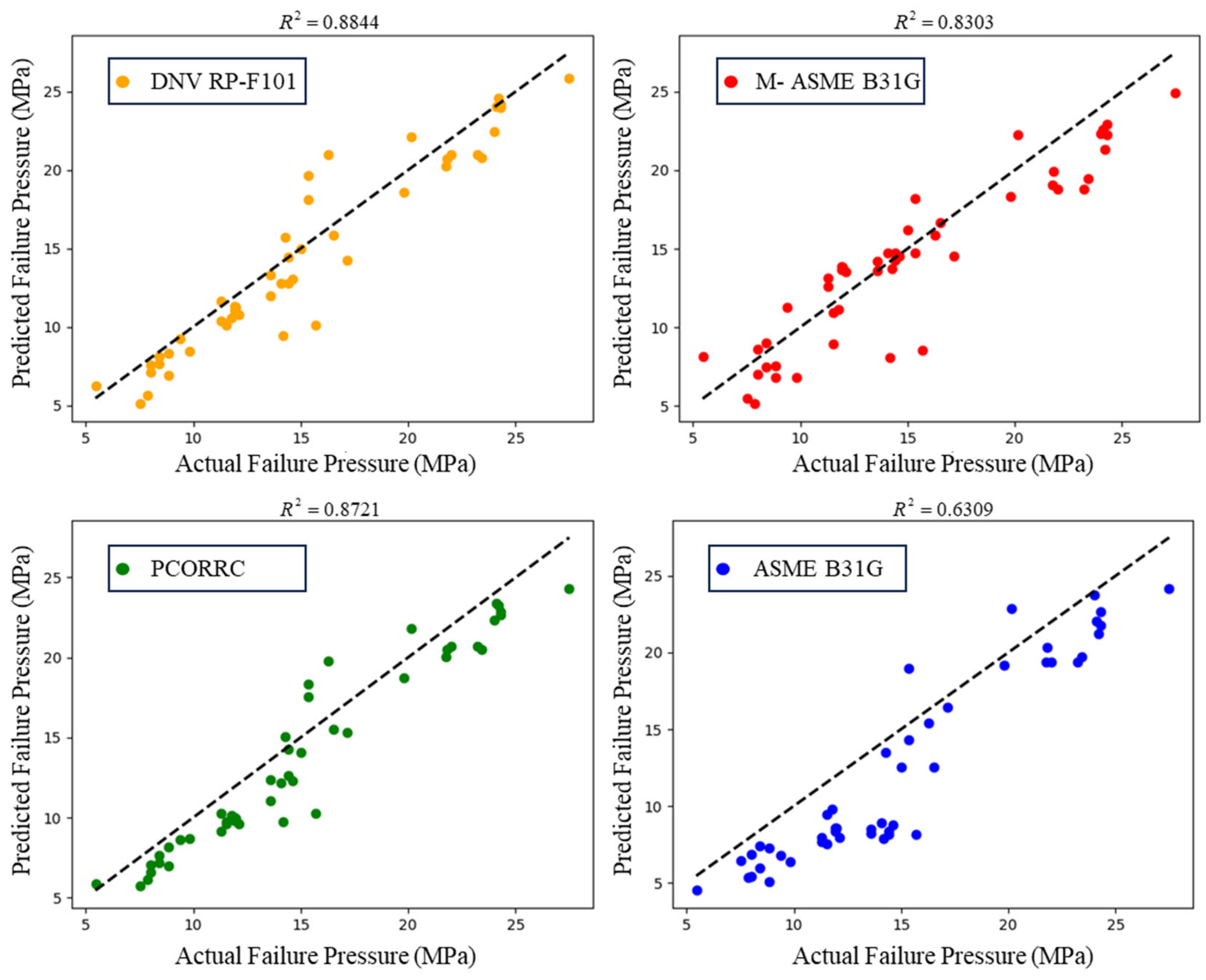
In this study, we examined four classical empirical formulas, namely, ASME B31G, Modified ASME B31G, PCORRC Criteria, and DNV RP-F101, to determine the most suitable one for our dataset. Figure 2 illustrates the coefficients of determination (R2) between the predicted failure pressures and the actual failure pressures for each of these formulas on the training dataset. Among them, (a) DNV RP-F101 exhibited the best predictive performance with an R2 value of 0.8844. This indicates a strong correlation between the predicted and actual failure pressures for this formula. The next best performance was observed with (c) PCORRC Criteria, which had an R2 value of 0.8721, suggesting a slightly lower but still substantial correlation. The Modified ASME B31G, represented by (b), achieved an R2 value of 0.8303, indicating a good but less accurate fit compared to the first two formulas. Finally, the original ASME B31G, shown in (d), had the lowest R2 value of 0.6309, indicating a weaker correlation between the predicted and actual failure pressures. Based on these results, we concluded that DNV RP-F101 is the most appropriate empirical formula for our dataset due to its superior predictive accuracy.
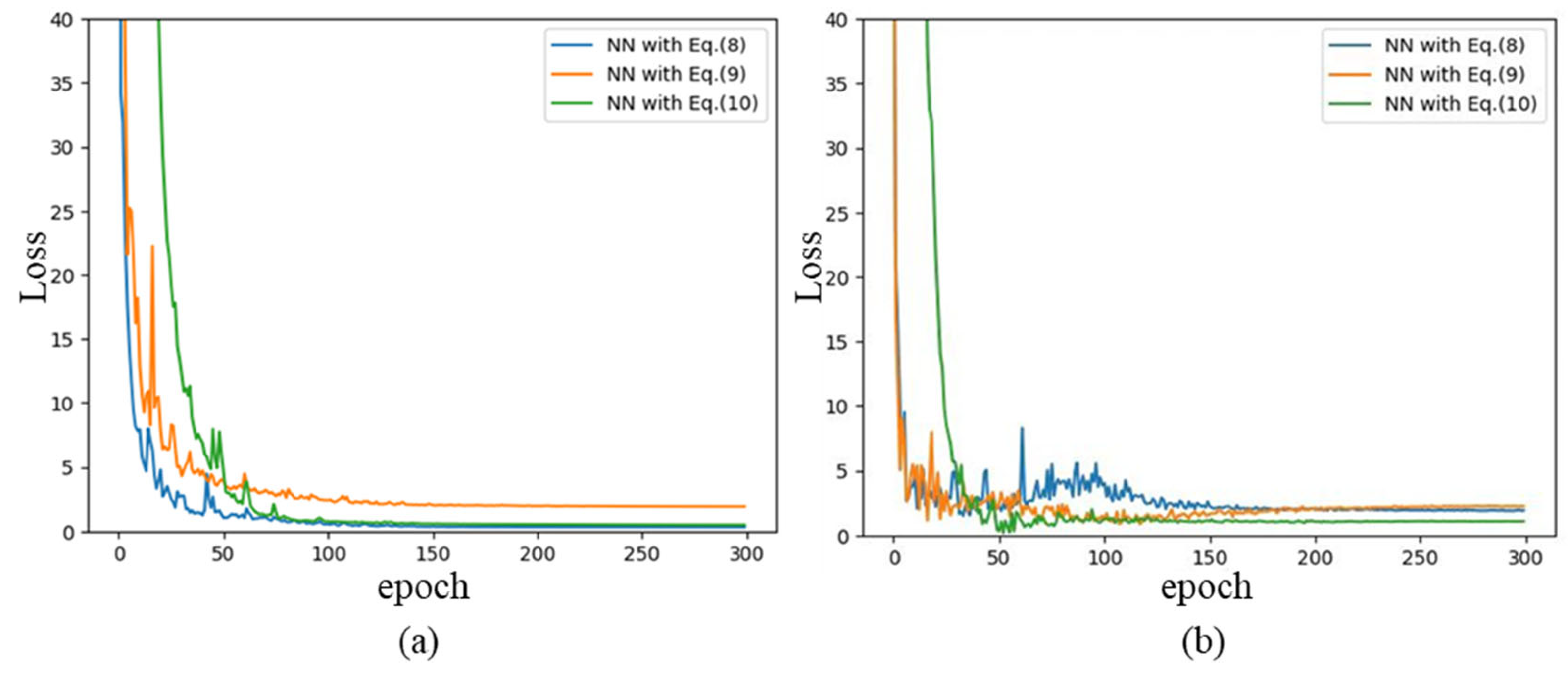
To compare the impact of different loss functions on the optimization of neural networks, this study trained three distinct neural network models using the loss functions defined in Equations (8)–(10). Specifically, Equation (8) represents a loss function supervised by actual failure pressure, which relies solely on the observed failure pressure data to guide the training process. Equation (9) builds upon this foundation by incorporating an empirical formula-induced term, meaning that the loss is calculated directly by comparing the predicted failure pressure with the empirical formula. In contrast, Equation (10) introduces an additional term predicted by the neural network itself, which aims to compensate for the deficiencies of the empirical formula. Figure 3a presents the variation of the loss functions for each model during the training process as a function of the number of iterations. All models tend to converge around 120 epochs. However, the model trained with Equation (9) converged a final loss value that is significantly higher than those of the other two models, indicating a less efficient optimization outcome. Figure 3b illustrates the variation of the loss function during the validation process. In the initial 100 epochs, the loss function exhibited significant oscillations for all models. The model trained with Equation (8) demonstrated a relatively slow convergence rate, eventually stabilizing around the 120th epoch. In contrast, the models using Equations (9) and (10) converged more rapidly, reaching stability around the 80th epoch. Notably, the model trained with Equation (9) achieves a final loss value that is higher than those of the other two models, which is consistent with the training results.
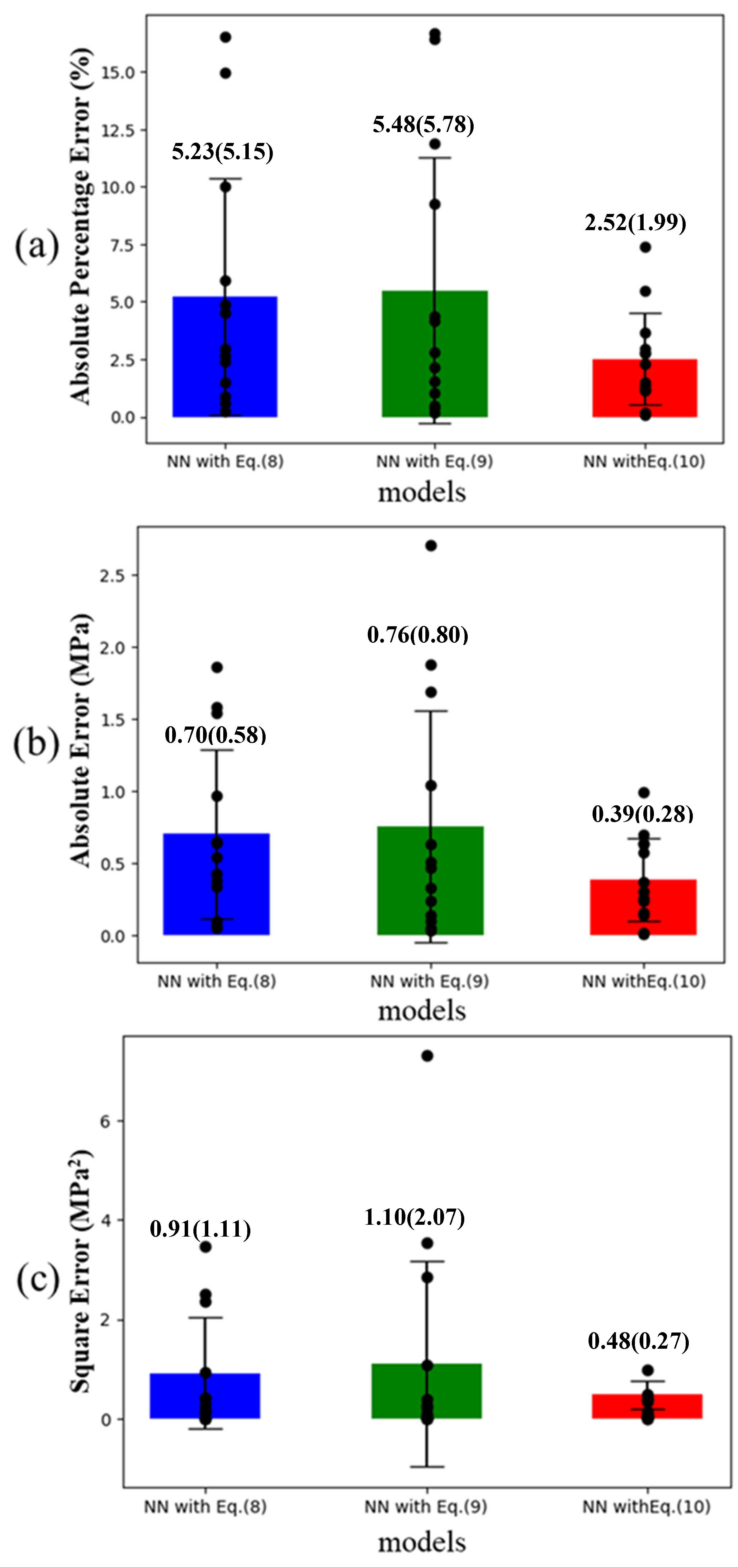
To validate the performance of the models, this paper statistically analyzed the prediction errors of the models. Figure 4 presents the three types of statistical errors for each model in the form of bar charts with data distributions. Specifically, Figure 4a shows the absolute percentage error (APE) of the predictions, which reflects the proportion of prediction errors relative to the true values. Figure 4b illustrates the absolute error (AE), indicating the magnitude of the deviation between the predicted and actual values. Figure 4c displays the squared error (SE), which highlights samples with large prediction errors. The numbers on top of the bars represent the average values of the respective bars, with (a), (b), and (c) corresponding to the mean absolute percentage error (MAPE), mean absolute error (MAE), and mean squared error (MSE), respectively. The values in parentheses are the standard deviations. From the average error values shown in Figure 4, it can be observed that overall, the third model outperforms the first two models. The prediction errors of the first model are slightly higher than those of the third model. However, the second model has some samples with significant deviations from the actual values, which is the primary reason for its higher prediction errors compared to the first model. This is attributed to the second model′s direct use of an imprecise empirical formula to calculate the results and compute the loss, making it more sensitive to changes in corrosion defect sizes and less adaptable to various defect scenarios. In contrast, the third model employs an improved empirical formula as part of the loss function calculation, enhancing its adaptability to different defect conditions.
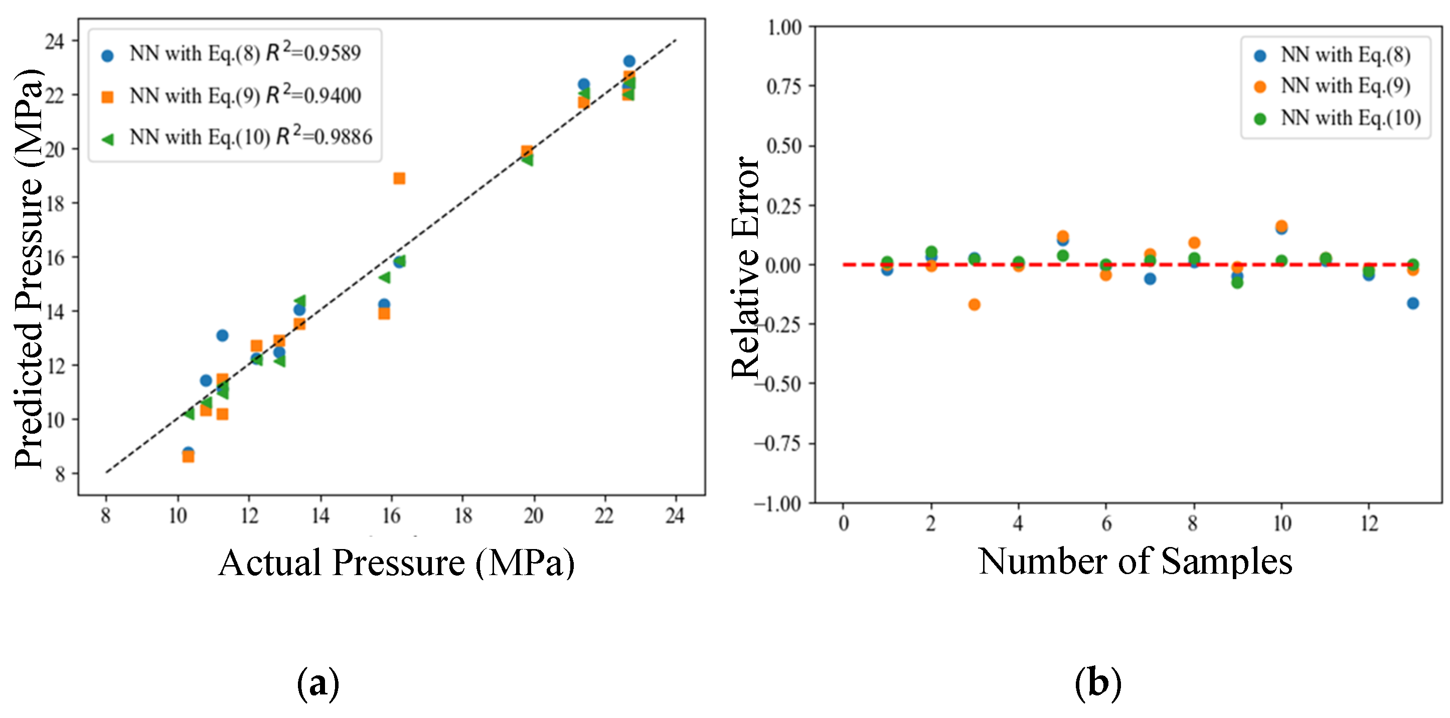
Next, this study compares the prediction results and their errors among samples across three models. Figure 5 presents the prediction results of different models on each sample in the validation set. Specifically, Figure 5a provides an intuitive comparison of the deviations between predicted and actual values by plotting the predicted values against the true values. The coefficient of determination (R2) for each model is indicated in the legend. Meanwhile, Figure 5b visually illustrates the positive and negative deviations of the prediction results for each sample. Table 2 lists the numerical deviations of prediction results for each sample across the models. From Figure 5a, it is evident that the third model achieves the highest coefficient of determination (R2 = 0.9886), followed by the first model (R2 = 0.9589), which is slightly higher than the second model (R2 = 0.9400). Table 2 reveals that the second model exhibits significantly smaller errors in predicting the failure pressures of samples 1, 2, 4, and 9, while its predictions for samples 3 and 10 are notably larger. This trend is similar to the deviations observed when using the empirical formula DNV RP-F101 for failure pressure prediction. This suggests that the direct incorporation of empirical-formula-calculated failure pressures into the loss function (second model) may cause the model to overfit to defect scenarios that align with the empirical formula, while increasing the deviations for other cases. In contrast, the model trained with the improved loss function (third model) shows a significant improvement in overfitting. This third model exhibits stronger adaptability to various defect scenarios, thereby providing more accurate and robust predictions across the validation set.

5. Conclusions

In conclusion, this study proposes an innovative method for predicting the failure pressure of corroded pipelines by integrating empirical formulas into the loss function of a neural network model. The proposed approach effectively combines the strengths of empirical formulas and artificial neural networks, leveraging the instructive nature of empirical knowledge while benefiting from the powerful fitting capabilities of ANNs. The integration of an additional defect factor term in the loss function allows for the model to compensate for errors caused by varying defect conditions, thereby enhancing its adaptability and accuracy across diverse corrosion scenarios. The results demonstrate that the proposed method outperforms traditional empirical formulas and ANN models trained with standard loss functions, achieving a mean absolute percentage error (MAPE) of 2.52%, a root mean square error (RMSE) of 0.39 MPa, and a coefficient of determination (R2) of 0.9886 on the validation set. This study highlights the importance of integrating empirical knowledge with data-driven models to improve prediction accuracy and robustness. The proposed method provides a simple yet effective solution for predicting the failure pressure of corroded pipelines, contributing to enhanced pipeline integrity assessment and safety management. Future work may focus on further optimizing the model architecture and exploring additional empirical formulas to further improve the prediction performance. However, the empirical formula used in the proposed method has a significant impact on prediction accuracy. Generally, the better the fit of the empirical formula to the data, the higher the accuracy of the model trained using the proposed method. Additionally, the proposed approach could be extended to other engineering applications where empirical formulas and data-driven models can be effectively combined to address complex prediction tasks.

Author Contributions

Conceptualization, X.M.; Methodology, H.L. and X.M.; Software, H.L.; Formal analysis, H.L.; Resources, H.L.; Writing—original draft, H.L.; Writing—review & editing, H.L.; Visualization, X.M.; Supervision, X.M.; Project administration, X.M. All authors have read and agreed to the published version of the manuscript.

Funding

This research received no funding.

Data Availability Statement

The original contributions presented in this study are included in the article, further inquiries can be directed to the corresponding author.

Conflicts of Interest

Author Hongbo Liu was employed by the company Shannxi Provincial Natural Gas Co., Ltd. The remaining authors declare that the research was conducted in the absence of any commercial or financial relationships that could be construed as a potential conflict of interest.

References

  1. Mousavi, S.S.; Moghaddam, A.S. Failure pressure estimation error for corroded pipeline using various revisions of ASME B31G. Eng. Fail. Anal. 2020, 109, 104284. [Google Scholar] [CrossRef]
  2. Arumugam, T.; Karuppanan, S.; Ovinis, M. Finite element analyses of corroded pipeline with single defect subjected to internal pressure and axial compressive stress. Mar. Struct. 2020, 72, 102746. [Google Scholar] [CrossRef]
  3. O’Grady, T.; Hisey, D.; Kiefner, J. Pressure calculation for corroded pipe developed. Oil Gas J. 1992, 90, 442. [Google Scholar]
  4. Su, Y.; Li, J.F.; Yu, B.; Zhao, Y.L.; Yao, J. Fast and accurate prediction of failure pressure of oil and gas defective pipelines using the deep learning model. Reliab. Eng. Syst. Saf. 2021, 216, 108016. [Google Scholar] [CrossRef]
  5. Li, M.Z.; Liu, Z.Y.; Zhao, Y.; Zhou, Y.; Huang, P.; Li, X.; Li, P.L.; Wang, X.; Zhang, D.P. Effects of corrosion defect and tensile load on injection pipe burst in CO2 flooding. J. Hazard. Mater. 2019, 366, 65–77. [Google Scholar] [CrossRef]
  6. Belachew, C.T.; Lsmail, M.; Karuppanan, S. Burst Strength Analysis of Corroded Pipelines by Finite Element Method. J. Appl. Sci. 2011, 1845, 1850. [Google Scholar] [CrossRef]
  7. Silva, R.C.C.; Guerreiro, J.N.C.; Loula, A.F.D. A study of pipe interacting corrosion defects using the FEM and neural networks. Adv. Eng. Softw. 2007, 38, 868–875. [Google Scholar] [CrossRef]
  8. Kumar, S.D.V.; Lo, M.; Karuppanan, S.; Ovinis, P. Empirical Failure Pressure Prediction Equations for Pipelines with Longitudinal Interacting Corrosion Defects Based on Artificial Neural Network. Mar. Sci. Eng. 2022, 10, 764. [Google Scholar] [CrossRef]
  9. Xu, W.Z.; Li, C.B.; Choung, J.; Lee, J.M. Corroded pipeline failure analysis using artificial neural network schemes. Adv. Eng. Softw. 2017, 112, 255–266. [Google Scholar] [CrossRef]
  10. Chen, Z.; Li, X.; Wang, W.; Li, Y.; Shi, L.; Li, Y. Residual strength prediction of corroded pipelines using multilayer perceptron and modified feedforward neural network. Reliab. Eng. Syst. Saf. 2023, 231, 108980. [Google Scholar] [CrossRef]
  11. Xie, L.; Hbrekke, S.; Liu, Y.; Lundteigen, M.A. Operational data-driven prediction for failure rates of equipment in safety instrumented systems: A case study from the oil and gas industry. J. Loss Prev. Process Ind. 2019, 60, 96–105. [Google Scholar] [CrossRef]
  12. Canonaco, G.; Roveri MAlippi, C.; Podenzani, F.; Bennardo, A.; Conti, M.; Mancini, N. A transfer-learning approach for corrosion prediction in pipeline infrastructures. Appl. Intell. 2022, 52, 7622–7637. [Google Scholar] [CrossRef]
  13. Cai, B.P.; Zhang, Y.P.; Yuan, X.B.; Gao, C.T.; Liu, Y.H.; Chen, G.M.; Liu, Z.K.; Ren-Jie, J.I. A Dynamic-Bayesian-Networks-Based Resilience Assessment Approach of Structure Systems: Subsea Oil and Gas Pipelines as A Case Study. China Ocean. Eng. 2020, 34, 597–607. [Google Scholar] [CrossRef]
  14. Ma, Y.L.; Zheng, J.Q.; Liang, Y.T.; Klemeš, J.J.; Du, J.; Liao, Q.; Lu, H.F.; Wang, B.H. Deeppipe: Theory-guided neural network method for predicting burst pressure of corroded pipelines. Process Saf. Environ. Prot. 2022, 162, 595–609. [Google Scholar] [CrossRef]
  15. Chouchaoui, B. Evaluating the Remaining Strength of Corroded Pipelines; University of Waterloo: Waterloo, Canada, 1994. [Google Scholar]
  16. Kiefner, J.F.; Vieth, P.H. A Modified Criterion for Evaluating the Remaining Strength of Corroded Pipe; Battelle Columbus Div.: Columbus, OH, USA, 1989. [Google Scholar]
  17. Stephens, D.R.; Leis, B.N. Development of an Alternative Criterion for Residual Strength of Corrosion Defects in Moderate to High Toughness Pipe. In Proceedings of the 2000 3rd International Pipeline Conference, American Society of Mechanical Engineers Digital Collection, Calgary, AB, Canada, 1–5 October 2000. [Google Scholar] [CrossRef]
  18. Raissi, M.; Perdikaris, P.; Karniadakis, G.E. Physics-informed neural networks: A deep learning framework for solving forward and inverse problems involving nonlinear partial differential equations. J. Comput. Phys. 2019, 378, 686–707. [Google Scholar] [CrossRef]
  19. Gao, J.; Yang, P.; Li, X.; Zhou, J.; Liu, J.K. Analytical prediction of failure pressure for pipeline with long corrosion defect. Ocean. Eng. 2019, 191, 106497. [Google Scholar] [CrossRef]
  20. Freire, J.L.F.; Vieira, R.D.; Castro, J.T.P.; Benjamin, A.C. Part 3: Burst tests of pipeline with extensive longitudinal metal loss. Exp. Tech. 2017, 30, 60–65. [Google Scholar] [CrossRef]
  21. Mok, D.H.B.; Pick, R.J.; Glover, A.G.; Hoff, R. Bursting of line pipe with long external corrosion. Int. J. Press. Vessel. Pip. 1991, 46, 195–216. [Google Scholar] [CrossRef]
  22. Kim, Y.; Kim, W.; Lee, Y.; Oh, K. The Evaluation of Failure Pressure for Corrosion Defects Within Girth or Seam Weld in Transmission Pipelines. In Proceedings of the 2004 International Pipeline Conference, American Society of Mechanical Engineers Digital Collection, Calgary, AB, Canada, 4–8 October 2004; pp. 1847–1855. [Google Scholar] [CrossRef]
  23. Chen, J.X.; Li, A.Z.; Yang, Q.K.; Lin, C.; Ren, Y.C.; Jin, S.R.; Li, C.C.; Qi, M. Novel In0.49Ga0.51P/(In)GaAs/GaAs p-type modulation doped heterostructure grown by gas source molecular beam epitaxy. J. Cryst. Growth 1998, 193, 28–32. [Google Scholar] [CrossRef]
  24. Shuai, Y.; Shuai, J.; Liu, C.Y. Research on the reliability methods of corroded pipeline. Pet. Sci. Bull. 2017, 2, 288–297. [Google Scholar]
  25. Mannucci, G.; Demofonti, G. Fracture Properties of API X 100 Gas Pipeline Steels; Europipe: Mülheim an der Ruhr, Germany, 2002; pp. 1–128. [Google Scholar]
  26. Wu, H.; He, K.M. Group Normalization. Int. J. Comput. Vis. 2019, 128, 742–755. [Google Scholar] [CrossRef]
  27. Xiao, R.; Zayed, T.; Meguid, M.A.; Sushama, L. Predicting failure pressure of corroded gas pipelines: A data-driven approach using machine learning. Process Saf. Environ. Prot. 2024, 184, 1424–1441. [Google Scholar] [CrossRef]
  28. Li, Y.; Chen, Z.F.; Wang, W.; Han, K.; Shuai, Y.; Wang, G.X. A novel assessment method for residual strength of CO2 pipelines with multiple defects based on RF-MLP. Reliab. Eng. Syst. Saf. 2025, 261, 111088. [Google Scholar] [CrossRef]
  29. Xu, L.; Wen, S.; Huang, H.; Tang, Y.; Wang, Y.; Pan, C. Corrosion failure prediction in natural gas pipelines using an interpretable XGBoost model: Insights and applications. Energy 2025, 325, 136157. [Google Scholar] [CrossRef]
  30. Lu, H.; Peng, H.; Xu, Z.D.; Qin, G.; Azimi, M.; Matthews, J.C.; Cao, L. Theory and Machine Learning Modeling for Burst Pressure Estimation of Pipeline with Multipoint Corrosion. J. Pipeline Syst. Eng. Pract. 2023, 14, 1481. [Google Scholar] [CrossRef]
  31. Xu, L.; Wang, Y.; Mo, L.; Tang, Y.; Wang, F.; Li, C. The research progress and prospect of data mining methods on corrosion prediction of oil and gas pipelines. Eng. Fail. Anal. 2023, 144, 106951. [Google Scholar] [CrossRef]
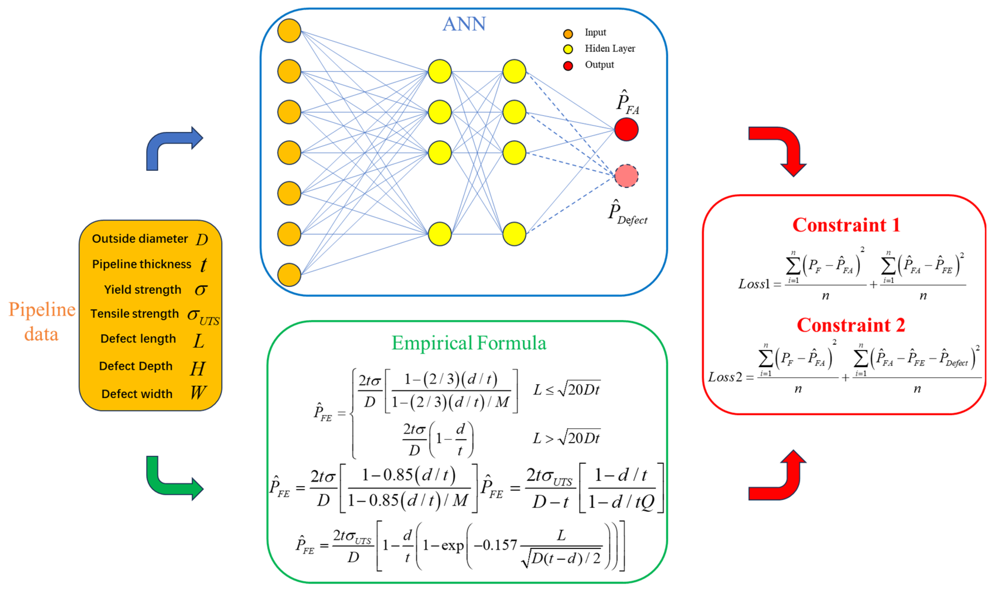
Figure 1. Empirical formula-constrained optimization for predicting failure pressure in corroded pipelines.
Applsci 15 05787 g001
Figure 2. Coefficient of determination between actual failure pressure and predicted failure pressure from empirical formulas.
Applsci 15 05787 g002
Figure 3. The loss of different models various with iterations. (a) is the training process while (b) is the validation process.
Applsci 15 05787 g003
Figure 4. Statistical results of predictions by different models on the validation set. (a) shows the absolute percentage error of different models, (b) shows the absolute error of different models, and (c) shows the square error. The numbers above the bars represent the average error across all samples, with the corresponding values in parentheses indicating the standard deviation.
Applsci 15 05787 g004
Figure 5. Prediction results of different models on each sample in the validation set. (a) is a scatter plot of the predicted and actual values for each sample, with the legend indicating the corresponding coefficient of determination. (b) is the error between the predicted and actual values for each sample.
Applsci 15 05787 g005
Table 1. The details of 60 samples from various literature sources.
LiteratureMaterialsPFDtLHWσσUTS
(Freire et al., 2006) [20]X8022.68458.88.139.65.3931.9601684
X8024.2459.4840.053.7532589730.5
X6014.4323.99.8255.67.0895.3452542
X6014.07323.99.66305.66.7695.3452542
X6013.58323.99.713506.9395.3452542
X6012.84323.99.71394.56.9195.3452542
X6012.13323.99.91433.47.3195.3452542
X6011.92323.99.74466.77.0295.3452542
X6011.91323.99.79488.76.9995.3452542
X6011.99323.99.795006.9995.3452542
X6011.3323.99.74527.87.1495.3452542
X6014.650814.650010.3597478600
X6013.450814.350010.397478600
X6015.850814.85009.797478600
X469.476.22751.416391458
A255.4576.22.04751.4416260309
(Mok et al., 1991) [21]X6011.255086.63812.6225.4540610.3
X6085086.359003.4325.4540610.3
X6011.85086.359002.1625.4540610.3
X608.45086.3510003.1825.4540610.3
X6011.555086.710162.6625.4540610.3
(Kim et al., 2008) [22]X6527.576217.5508.7550495565
X6524.376217.51008.7550495565
X6521.876217.52008.7550495565
X6519.876217.53008.7550495565
X6516.576217.56008.7550495565
X651576217.59008.7550495565
X6524.1176217.52004.250474.1556.6
X6521.7676217.52008.950474.1556.6
X6517.1576217.520013.150474.1556.6
X6524.376217.51008.450474.1556.6
X6519.876217.53008.550474.1556.6
X6523.4276217.52008.4100474.1556.6
X6522.6476217.52009200474.1556.6
(Chen et al., 1998) [23]20F10.84266.951602.725240390
20F9.8142671503.821240390
20F7.8542671505.225240390
208.8352993504.725285415
2015.752991604.725285415
2014.252991505.325285415
X6010.372081804.325425535
X608.8372083204.426425535
X607.5572081806.226425535
(Shuai et al., 2017b) [24]-15.36304.86.35264.9520351543
-16.29304.86.35334.2521382570
-14.29304.86.35374.6430351463
-16.223246.0119.353.619382570
-23.232410.32435.15154.5380514
-2232410.32435.1530.9380514
-11.255086.63812.6225.4443.4598.9
-85086.359003.4325.4429.6572.5
-8.45086.3510003.1825.4434.8572.5
-11.555086.710162.6625.4430601
-14.4323.99.8255.66.9595.3422.5589.6
-13.58323.99.713506.8595.3422.5589.6
-12.19323.99.91433.47.0895.3422.5589.6
(Mannucci and Demofonti, 2002) [25]X10015.351422.419.2518010.40.5740774
X10020.121422.420.13853.80.5795840
X10021.4914.416.415090.5739813
X10024.02914.416.445060.5739813
Table 2. The detail comparison of prediction results of different models on the validation set.
NumberPFDNV RP-F101NN with Equation (8)NN with Equation (9)NN with Equation (10)
P ^ F E Re (%) P ^ F A Re (%) P ^ F A Re (%) P ^ F A Re (%)
122.6821.98−3.0923.22+2.3722.64−0.1722.42−1.15
212.8411.72−8.7212.46−2.9712.89+0.4112.14−5.42
316.2220.67+27.4415.79−2.6518.92+16.6415.85−2.28
419.8018.59−6.1119.75−0.2419.90+0.5019.56−1.22
515.8015.41−2.4714.22−10.0113.92−11.8915.22−3.69
612.1912.70+4.1812.26+0.5412.70+4.1412.20+0.05
710.809.92+8.1511.44+5.9310.33−4.3510.64−1.51
811.2510.62+5.6011.15−0.8810.21−9.2410.94−2.75
913.4012.32+8.0614.05+4.8313.54+1.0314.39+7.37
1010.308.23+20.108.76−14.958.61−16.4510.16−1.33
1122.6420.18+10.8722.30−1.5122.01−2.7922.00−2.82
1221.4024.51+14.5322.37+4.5321.73+1.5522.03+2.96
1311.2510.82+3.8213.11+16.5411.49+2.1211.23−0.22
Disclaimer/Publisher’s Note: The statements, opinions and data contained in all publications are solely those of the individual author(s) and contributor(s) and not of MDPI and/or the editor(s). MDPI and/or the editor(s) disclaim responsibility for any injury to people or property resulting from any ideas, methods, instructions or products referred to in the content.