Refined Consolidation Settlement Calculation Based on the Oedometer Tests for Normally and Overconsolidated Clays

Abstract

This study presents an enhanced analytical approach for one-dimensional consolidation settlement by introducing a revised AJOP (arc joint via optimum parameters) equation assuming creep and strain rate effects can be neglected for both normally and overconsolidated clays. This modified equation integrates both curved and linear segments within a unified framework, enhancing accuracy across varying stress levels for normally consolidated clay. Additionally, the revised AJOP function, coupled with newly proposed equations for symmetrical and asymmetrical hysteresis, improves the modeling of overconsolidated clay. The findings from a comparative investigation using benchmark datasets and conventional methods, including the linear function (LF) and the curved function (CF), reveal that the revised AJOP method was found to reduce settlement prediction errors by up to 85% compared to LF method (particularly at shallow layers) and by 10–15% compared to the CF method (particularly at deep layers). The revised AJOP equation effectively resolves this error with a wide range of depths. Furthermore, results highlight the crucial impact of clay layering techniques on consolidation settlement predictions. Non-layered models yield lower settlement estimates compared to multilayer approaches, emphasizing the significance of the proper $e-log{{\mathsf{\sigma }}^{\prime }}_v$ relationship and layering techniques in enhancing prediction reliability.

1. Introduction

Consolidation settlement is a crucial factor in the total settlement of clayey soils. If excessive, it can cause structural damage. This type of settlement occurs gradually as pore water dissipates from soil voids under applied loads, resulting in time-dependent deformation. It is crucial to predict the consolidation settlement with high accuracy, otherwise the error of the calculation can result in considerable post-construction settlement and high maintenance costs. In the literature, the method for calculating the consolidation settlement of clay at any given time after the application of a load can be calculated using the formula $\rho ={\rho }_t·U$ where ρ represents the consolidation settlement at any time $t$ occurred after the load is applied, ${\rho }_t$ is the total consolidation settlement, and U is the degree of consolidation. In order to calculate ρ precisely, accurate values for both ${\rho }_t$ and U are required.

For the calculation of U, the nonlinear consolidation theory was first proposed by Davis and Raymond [1]. It is predicted on the assumptions that the initial effective stress remains constant with depth and the permeability is proportional to the compressibility during the consolidation process [2,3], which limit applicability in heterogeneous soil profiles. Numerous attempts have been made to create various one-dimensional consolidation models that take into account the nonlinear variations in permeability and compressibility [4,5,6,7,8,9,10,11,12,13,14,15,16,17,18,19,20]. Recently, Kim et al. (2021) [21] successfully developed the analytical solution for U of multilayered soil under time-dependent loading. Based on this information, the calculation of U therefore has high accuracy. On the other hand, in the literature, the calculation of ${\rho }_t$ still relies on an approximation method. This method is based on a linear relationship between the void ratio ($e$) and effective vertical stress ($log{{\sigma }^{\prime }}_v$) derived from the one-dimensional consolidation tests conducted in the laboratory. In soil mechanics, two types of clay are explained via $e-log{{\sigma }^{\prime }}_v$: normally consolidated clay (NC), which is clay where the current stress is the highest it has ever been, and overconsolidated clay (OC), which is clay that has experienced higher stress in the past than the current stress (e.g., [22,23,24]). The virgin compression line (VCL) is defined as the portion of the graph that represents NC. Additionally, in the experiment, there will be parts of the graph showing unloading and reloading portions (referred as the hysteresis); both of them represent OC. Although the test results are nonlinear, the calculation method assumes linear approximation for both the VCL and the hysteresis for simplicity. The equations used to calculate consolidation settlement based on this approximation, which applies to the difference in void ratio ($\mathit{\Delta }e$) from the experimental result graphs, are presented in Equations (1) and (2) (e.g., [25]). This approximation contributes to the ongoing inaccuracy in calculating consolidation settlement ${\rho }_t$ and ρ.

Normally consolidated clay:

$$\rho =H\left[{\displaystyle \frac{\mathit{\Delta }e}{1+e_0}}\right]={\displaystyle \frac{H}{1+e_0}}\left[C_{c}log\left({\displaystyle \frac{{{\sigma }^{\prime }}_{v0}+\mathit{\Delta }\sigma }{{{\sigma }^{\prime }}_{v0}}}\right)\right]$$

(1)

Overconsolidated clay:

$$\rho =H\left[{\displaystyle \frac{\mathit{\Delta }e}{1+e_0}}\right]={\displaystyle \frac{H}{1+e_0}}\left[C_r\mathit{log}\left({\displaystyle \frac{{{\sigma }^{\prime }}_p}{{{\sigma }^{\prime }}_{v0}}}\right)+C_{c}log\left({\displaystyle \frac{{{\sigma }^{\prime }}_{v0}+\mathit{\Delta }\sigma }{{{\sigma }^{\prime }}_p}}\right)\right]$$

(2)

In Equations (1) and (2), $H$ is the soil layer’s thickness, $e_0$ is the initial void ratio, ${{\sigma }^{\prime }}_{v0}$ is the effective overburden stress, ${{\sigma }^{\prime }}_p$ is the maximum past pressure, and $\mathit{\Delta }\sigma$ is the stress increment due to surface loading.

To address the inaccuracies in calculating consolidation settlement, it is essential to use appropriate equations for the $e-log{{\sigma }^{\prime }}_v$ curve rather than relying on linear approximations. In literature, the relationship between $e$ and $log \left(p\right)$, where $p$ represents the mean effective stress, from one-dimensional consolidation tests is frequently utilized for modeling soils, including clay (e.g., [26,27,28,29,30,31,32]) and sand (e.g., [33,34,35,36,37,38,39]). A comprehensive review by Kaewhanam and Chaimoon (2023) [40] found that linear equations are accurate for high stress levels but tend to be quite inaccurate at lower stress levels due to the curved nature of experimental results. In contrast, curved equations in the form of power functions, which are commonly used for granular soils, are accurate at lower stress levels because the experimental results follow a similar tendency. However, power functions can be significantly inaccurate at high stress levels as they cannot accurately represent a straight line. Additionally, Kaewhanam and Chaimoon (2023) [40] were the first to introduce an equation that combines a curve with a straight line on a semi-logarithmic scale, using only four fitting parameters. This approach can significantly reduce errors in calculating the changes in void ratio ($\mathit{\Delta }e$) for normally consolidated clay (NC). However, for calculations involving overconsolidated clay (OC), a nonlinear hysteresis equation remains necessary.

Recent studies suggest that creep and consolidation can occur simultaneously [41,42,43,44], challenging earlier findings that creep follows consolidation [45,46]. However, these studies rely on linear consolidation principles, necessitating a refined framework that separates consolidation from creep before integration. Field experiments, such as the Väsby test fill in Sweden [47], confirm that consolidation and creep settlement occur concurrently, with creep continuing beyond primary consolidation. The key concerns are primarily due to creep, strain rate effects, and sample disturbance—not sensitivity alone. Leroueil et al. (1985) [48] addressed this issue by incorporating time and strain rate into the $e-log{{\sigma }^{\prime }}_v$ relationship, leading to a more consistent stress–strain correlation for sensitive clays.

This study developed a formulation based on existing experimental data for consolidation settlement (${\mathrm{\rho }}_t$) assuming negligible creep and strain rate effects for both NC and OC clays. To achieve this, we (1) refined Kaewhanam and Chaimoon’s (2023) [40] equation to better model the $e-log{{\sigma }^{\prime }}_v$ relationship for NC clays, and (2) introduced new equations to capture hysteresis behavior in OC clays. These refinements established a closed-form solution for $\mathit{\Delta }e$ during loading, eliminating errors in consolidation settlement calculations in Equations (1) and (2).

2. Derivation of $\mathit{e}-\mathit{l}\mathit{o}\mathit{g}{{\mathit{\sigma }}^{\prime }}_{\mathit{v}}$ Equations for Laboratory Test Results

In this section, two advanced equations for arcs representing $e-log{{\sigma }^{\prime }}_v$ were developed: one for the virgin compression line (VCL) and one for the hysteresis. The specifics are described as follows.

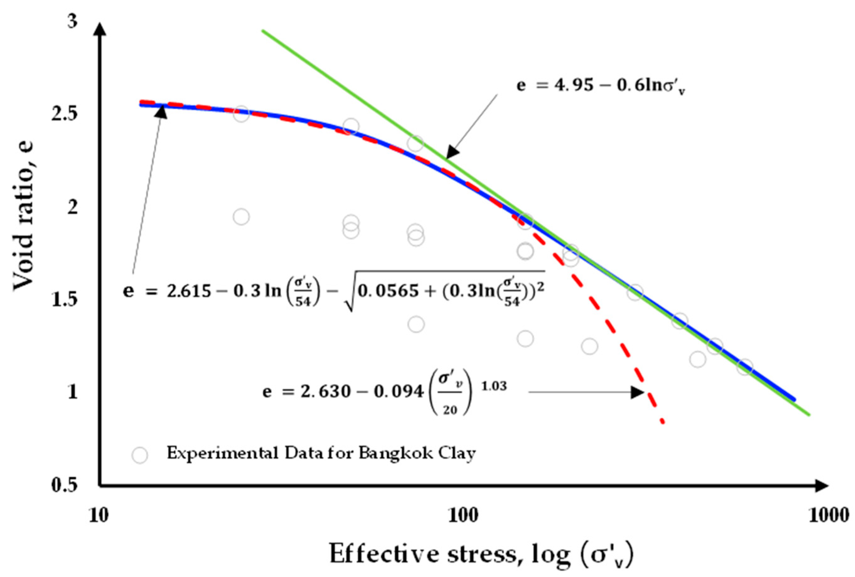
2.1. Equation for the Virgin Compression Line (VCL)

As previously mentioned, the equations for the virgin compression line (VCL) found in the literature include linear functions (LF) [26,27,28], curved functions (CF) [33,34,35,36,37,38,39], and combined linear-curved formulations, such as the equation proposed by Kaewhanam and Chaimoon (2023) [40], referred to here as the arc joint via optimum parameters (AJOP). These LF, CF, and AJOP equations describe the relationship between the void ratio ($e$) and the mean effective stress ($p^{\prime }$), where $p^{\prime }$ is defined as $({{\sigma }^{\prime }}_v+2{{\sigma }^{\prime }}_h)/3$ where ${{\sigma }^{\prime }}_v$ and ${{\sigma }^{\prime }}_h$ represent the effective vertical and horizontal stresses, respectively. The mathematical expressions for the LF, CF, and AJOP models are presented in Equations (3)–(5), and a comparison of their corresponding graphs is shown in Figure 1.

$$e=\Gamma -\lambda ·\mathit{ln}{p}^{\prime }$$

(3)

$$e=\Gamma -\lambda ·{\left({\displaystyle \frac{p^{\prime }}{{p^{\prime }}_a}}\right)}^{\xi }$$

(4)

$$e=\Gamma -\alpha ·ln\left({\displaystyle \frac{p^{\prime }}{{p^{\prime }}_{ref}}}\right)-\sqrt{\theta +{(\alpha ·ln\left({\displaystyle \frac{p^{\prime }}{{p^{\prime }}_{ref}}}\right))}^2}$$

(5)

Based on the graphical comparison shown in Figure 1 between LF, CF, and AJOP equations, the AJOP equation provides the most accurate representation of the e-lnp relationship across both low and high stress levels. In this study, the AJOP equation was adopted, and it was revised such that the independent variable (the variable on the horizontal axis of the graph) was made compatible with the consolidation test results. This aimed to simplify and streamline the calculation process. Thus, $p$ was changed to ${{\sigma }^{\prime }}_v$, the reference pressure ${p^{\prime }}_{ref}$ was changed to a reference positive value $R$, and the log was changed to the natural logarithm ln.

$$e=\Gamma -\alpha ·log\left({\displaystyle \frac{{{\sigma }^{\prime }}_v}{R}}\right)-\sqrt{\theta +{(\alpha ·log\left({\displaystyle \frac{{{\sigma }^{\prime }}_v}{R}}\right))}^2}$$

(6)

$${\overline{C}}_c=-{\displaystyle \frac{∆e}{∆log{{\sigma }^{\prime }}_v}}=\mathsf{\alpha }+\left\{\sqrt{\mathsf{\theta }+{\left(\mathsf{\alpha }\mathit{log}\left({\displaystyle \frac{{{\sigma }^{\prime }}_{v2}}{R}}\right)\right)}^2}-\sqrt{\mathsf{\theta }+{\left(\mathsf{\alpha }\mathit{log}\left({\displaystyle \frac{{{\sigma }^{\prime }}_{v1}}{R}}\right)\right)}^2}\right\}/log\left({\displaystyle \frac{{{\sigma }^{\prime }}_{v2}}{{{\sigma }^{\prime }}_{v1}}}\right)$$

(7)

Equation (6) presents the revised form of the AJOP function. The new fitting parameters of AJOP equation become Γ, $R$, $\alpha$, and $\theta$. According to the explanation in [40], Γ and $R$ control the vertical shift and the horizontal shift of the graph, respectively. While $\alpha$ controls the slope of the linear portion, $\theta$ controls the curvature of the curved portion. Here is a short guideline for determining parameters Γ, $R$, $\alpha ,$ and $\theta$. All four parameters Γ, $R$, $\alpha$, and $\theta$ are strictly positive. The parameter Γ acts as the upper bound of the void ratio and should be slightly greater than the maximum void ratio observed in the experimental data. The parameter R controls the horizontal position of the curve and can be initially set to atmospheric pressure (e.g., 101 kPa), with further adjustment of the remaining parameters as needed. However, all parameters can be freely adjusted to better fit the experimental results. Parameter $\alpha$ is typically close to half the slope of the linear function (LF) method. It is important to note that $\alpha$ equals exactly half the LF slope only when $\theta$ is set to zero. As for parameter $\theta$, initially it should be assumed as zero and gradually increased depending on the curvature of the dataset. A smaller curvature radius (i.e., sharper curve) requires a smaller $\theta$. A value of $\theta$ equal to zero corresponds to a sharp corner with no curvature. The sensitivity of parameters Γ, $R$, $\alpha ,$ and $\theta$ is summarized as follows.

(1)

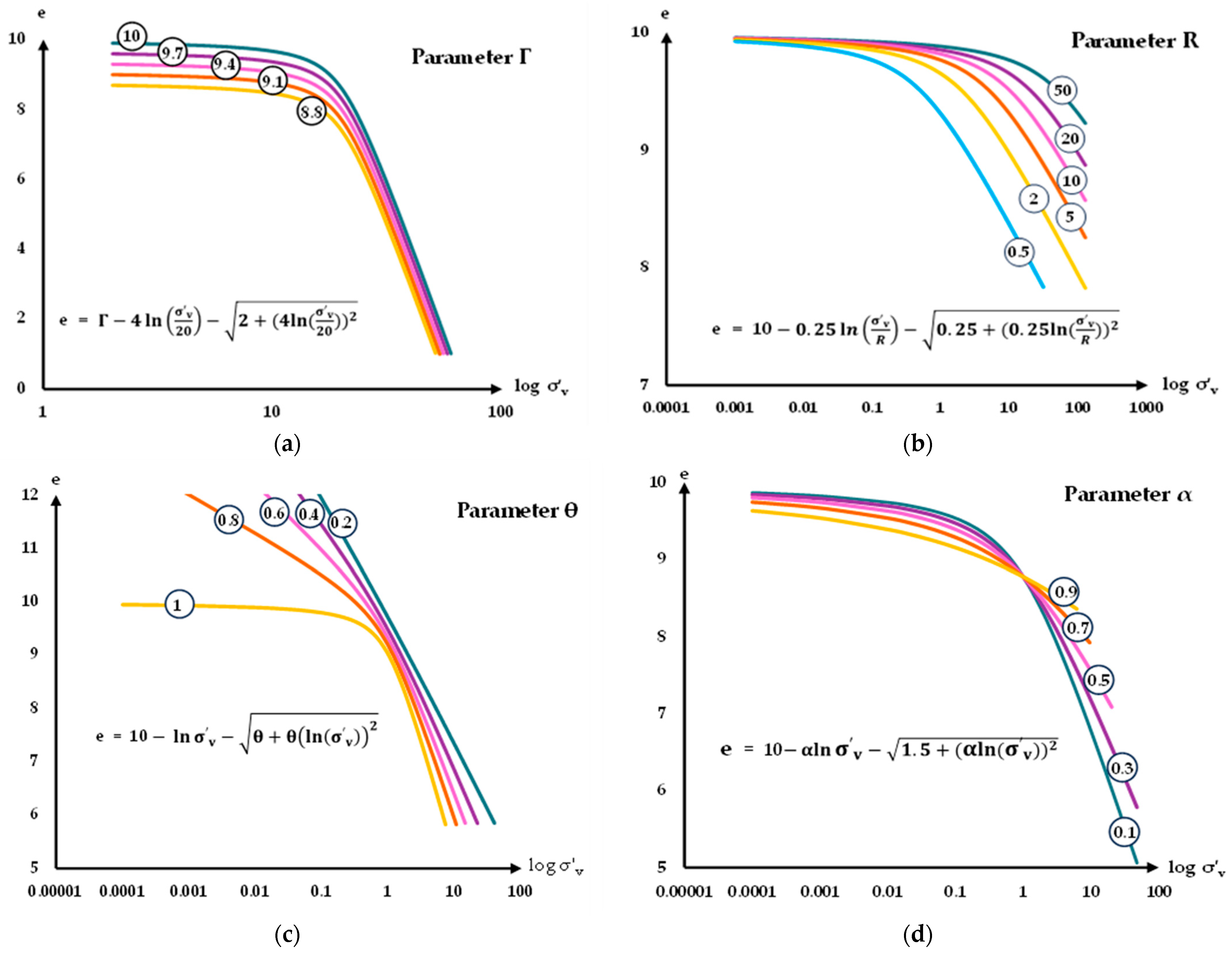
Parameter Γ primarily controls the asymptotic upper bound of the void ratio. As such, it has a strong influence on the vertical position of the curve at low stress levels. A small change in a affects the curve globally, particularly in the initial loading phase.

(2)

Parameter R governs the horizontal shift of the curve along the logarithmic stress axis. While its effect is not as dominant as that of α, it moderately influences the stress range at which transition between recompression and virgin compression occurs. Improper selection of R may cause a misalignment with the test data, especially in the mid-stress range.

(3)

Parameter $\alpha$ controls the slope of the curve in the virgin compression region. It exhibits high sensitivity in the high-stress domain, and an over- or underestimation of $\alpha$ can result in significant errors in predicted settlements, particularly for deeper soil layers or higher loads.

(4)

Parameter $\theta$ adjusts the degree of curvature of the curved portion of the virgin compression line. It is most sensitive in controlling the smoothness of the transition zone. A small change in $\theta$ can significantly alter the curvature behavior. When $\theta$ = 0, the model reduces to a piecewise function with a sharp corner; as $\theta$ increases, the transition becomes smoother, better capturing gradual changes in stiffness.

Due to the interdependency and nonlinear interaction among these parameters, a least-squares fitting procedure is recommended to optimize their values simultaneously. This enhances both the robustness and reproducibility of the model calibration process.

The secant slope $\overline{C_c}$ of the AJOP function can be determined using Equation (7). This equation provides an accurate calculation of $\mathit{\Delta }e$ between two points on VCL for normally consolidated clay without the estimation. Figure 2 shows the AJOP graph for the effects of various fitting parameters.

In Equation (7), ${{\sigma }^{\prime }}_{v1}$ and ${{\sigma }^{\prime }}_{v2}$ represent the vertical effective stresses at the initial point of stress interval (lower value) and the final point of interval (higher value), respectively, and ${{\sigma }^{\prime }}_{v2}>{{\sigma }^{\prime }}_{v1}$. The changes in $\mathit{\Delta }e$ between these two points can be calculated by multiplying $\overline{C_c}$ in Equation (7) by $\mathit{log}({{\sigma }^{\prime }}_{v2}/{{\sigma }^{\prime }}_{v1})$.

The application of the AJOP equation and its secant slope for calculating settlement in normally consolidated clays is straightforward. By substituting $C_c$ in Equation (1) with $\overline{C_c}$ in Equation (7), the errors in the calculation can be effectively eliminated across all soil depths. It is worth noting that the traditional method, which relies on linear approximation and a constant $C_c$, often results in significant calculation errors, particularly for shallow soils near the ground surface, and these errors tend to decrease with depth. This discrepancy arises because the initial stress near the surface is relatively low, resulting in the initial stress point, located on the curved portion of the $e-log{{\sigma }^{\prime }}_v$ rather than on the straight portion. In addition, the stress induced by the surface loads is comparatively higher when compared to deeper soil layers. Therefore, application of the LF causes a dramatic error of $\mathit{\Delta }e$. When comparing the capabilities of the AJOP and CF equations, it becomes evident that CF can address the aforementioned issues similarly to AJOP. However, the use of CF introduces significant computational errors at greater depths due to the absence of a linear segment in its graph. At these greater depths, the stress induced by surface loads is relatively minor, which implies that the resulting errors have less impact compared to those of LF at shallower depths.

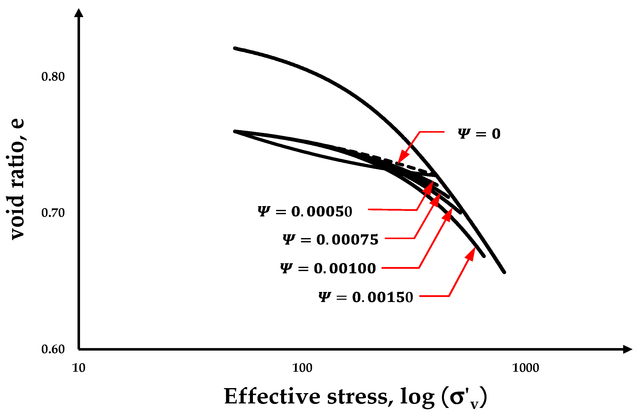
2.2. Equations for the Hysteresis

Hysteresis refers to a loop involving unloading followed by reloading in the consolidation test result of all clays due to the requirements in the experimental standard. This is to observe the reversible and irreversible deformation of clays during loading. In some clays, the unloading and reloading curves may overlap or closely align, allowing the hysteresis to be simplified using a straight line with a constant slope $C_r$. In such a situation, calculations using the linear approximation can provide accuracy for overconsolidated clays. However, some clays exhibit differently, such as clays in [22,23,24], where it is evident that the unloading and reloading curves deviated significantly. For these clays, the secant slope between two points on the unloading or reloading curves differed to the value of the average value $C_r$. Therefore, the existing linear approximation method cannot provide high accuracy for these clays. To address this, adopting an equation capable of representing both types of hysteresis behavior could improve the accuracy of settlement calculations in overconsolidated clays. This approach enhances the precision of modeling soil compression and helps in predicting deformation under varying loading conditions more reliably.

Additionally, it was found that some hysteresis can be both symmetric and asymmetric. Symmetric hysteresis refers to cases where the reloading curve returns a point close to the starting point of the unloading curve on VCL. However, certain clays exhibit different characteristics, specifically asymmetric hysteresis, where the reloading curve bends below the starting point of the unloading curve on VCL. This behavior contributes to the increased occurrence of irreversible strain in overconsolidated clays, which tend to experience greater water expulsion than usual.

$$e={\displaystyle \frac{{\left(log{{\sigma }^{\prime }}_v-h\right)}^2}{4C}}+k$$

(8)

It is necessary to consider both accuracy and ease of use in order to create equations that correctly depict the unloading–reloading part. In this study, parabolic equations are employed. Generally, three fitting parameters are used for a parabola, as shown in Equation (8). An upward-facing parabolic equation represents the unloading phase (with parameters $C$, $h$ and $k$), while a downward-facing parabolic equation represents the reloading phase of the experimental results (with different parameters $C_1$, $h_1$, and $k_1$). It should be noted that Equation (8) can be valid for the unloading only if ${{\sigma }^{\prime }}_v$ is less than or equal to the stress at the unloading point ${{\sigma }^{\prime }}_{\mathcal{v}}$ on VCL. Figure 3 illustrates the concept of using parabolas to describe the unloading–reloading graphs.

It is crucial to first formulate an equation to represent symmetric hysteresis behavior. Once this foundational equation is established, it can be further revised to accommodate asymmetric hysteresis. This approach ensures systematic progression from simpler to more complex representations of hysteresis, enhancing the ability to accurately model and predict soil behavior under varying conditions.

2.2.1. Equations for the Symmetric Hysteresis

For symmetric hysteresis, three parameters ($C$, $h$ and $k$) should be applicable to both the upward-facing and downward-facing parabolas for simplicity. Therefore, it is necessary to derive the values of $C_1$, $h_1$, and $k_1$ for the downward-facing parabola based on the values of $C$, $h$ and $k$ of the upward-facing parabola.

Based on Equation (8), which is the equation for the unloading curve, the change in void ratio $\Delta e$ and the secant slope $\overline{C_r}\left(Un\right)$ between the starting point of unloading (${{\sigma }^{\prime }}_{\mathcal{v}}$) and any point on the symmetrical unloading (${{\sigma }^{\prime }}_v$) can be calculated using Equations (9) and (10), respectively.

$$\mathit{\Delta }e=e-e_{\mathcal{v}}={\displaystyle \frac{{\left(\mathit{log}{{\sigma }^{\prime }}_v\right)}^2-{\left(\mathit{log}{{\sigma }^{\prime }}_{\mathcal{v}}\right)}^2-2h·\mathit{log}({{\sigma }^{\prime }}_v/{{\sigma }^{\prime }}_{\mathcal{v}})}{4C}}$$

(9)

$$\overline{C_r}\left(Un\right)=-{\displaystyle \frac{\mathit{\Delta }e}{\mathit{\Delta }log{{\sigma }^{\prime }}_v}}={\displaystyle \frac{2h-log\left({{\sigma }^{\prime }}_{\mathcal{v}}·{{\sigma }^{\prime }}_v\right)}{4C}}$$

(10)

In the case of symmetric hysteresis, the size of the upward parabolas used to represent the unloading and reloading curves is identical. Consequently, the parameter $C_1$ can be expressed in terms of $C$. Next, to determine the formulas for $h_1$ and $k_1$, it is necessary to set up two additional conditions. From Figure 3, it can be observed that the reloading line intersects two key points; i.e., the point where unloading begins $\left({{{\sigma }^{\prime }}_{\vartheta } , e}_{\vartheta }\right)$ and the point where reloading begins $\left({{{\sigma }^{\prime }}_{\omega } , e}_{\omega }\right)$. We use the coordinates of these two points to find $h_1$ and $k_1$. First, determine the void ratio $e$ at both points by substituting the stress ${{\sigma }^{\prime }}_{\vartheta }$ into the VCL equation (Equation (6)) to obtain $e_{\vartheta }=f\left(\Gamma ,R,\alpha ,\theta \right)$. Then, substitute the stress value at the reloading start point ${{\sigma }^{\prime }}_{\omega }$ into the unloading equation (Equation (8)) to obtain $e_{\omega }$. Using the condition that $C_1=-C$ for both calculations, by solving the simultaneous equations, we can derive formulas for $h_1$ and $k_1$ that depend on the four parameters of the newly proposed VCL ($\Gamma ,R,\alpha ,\theta )$, as well as $C$, $h$, and $k$. The equations for $C_1$, $h_1$ and $k_1$ of the downward-facing parabola are shown in Equations (11)–(13), respectively.

$$C_1=-C$$

(11)

$$h_1={\displaystyle \frac{4C_1\left(e_{\omega }-e_{\vartheta }\right)-{\left(log{{\sigma }^{\prime }}_{\omega }\right)}^2+{\left(log{{\sigma }^{\prime }}_{\vartheta }\right)}^2}{2\left(log{{\sigma }^{\prime }}_{\vartheta }-log{{\sigma }^{\prime }}_{\omega }\right)}}$$

(12)

$$k_1=e_{\omega }-{\displaystyle \frac{1}{4C_1}}{\left(log{{\sigma }^{\prime }}_{\omega }-h_1\right)}^2$$

(13)

where $e_{\vartheta }=f\left(\mathrm{\Gamma },R,\alpha ,\theta \right)=\mathrm{\Gamma }-\alpha ·log\left({\displaystyle \frac{{{\sigma }^{\prime }}_{\vartheta }}{R}}\right)-\sqrt{\theta +{\left(log\left({\displaystyle \frac{{{\sigma }^{\prime }}_{\vartheta }}{R}}\right)\right)}^2}$ and $e_{\omega }={\displaystyle \frac{{\left(log{{\sigma }^{\prime }}_{\omega }-h\right)}^2}{4C}}+k$.

At this step of the optimum parameter technique, a complete symmetric hysteresis (both unloading and reloading phases) can be evaluated using only three parameters ($C$, $h$ and $k$). Furthermore, the tangent slope $\kappa$ of the unloading portion in Equation (8) can be expressed in Equation (14). At the starting point of unloading (and on VCL), the tangent slope $\kappa$ is usually assumed to be a constant ${\kappa }_0$ for each type of soil. Therefore, ${\kappa }_0$ can be determined by substituting ${{\sigma }^{\prime }}_v$ in Equation (14) with ${{\sigma }^{\prime }}_{\vartheta }$ as shown in Equation (15).

$$\kappa ={\displaystyle \frac{de}{dlog{{\sigma }^{\prime }}_v}}={\displaystyle \frac{\left(log{{\sigma }^{\prime }}_v-h\right)}{2C}}$$

(14)

$${\kappa }_0={\displaystyle \frac{\left(log{{\sigma }^{\prime }}_{\vartheta }-h\right)}{2C}}$$

(15)

To calculate the $\kappa$ and ${\kappa }_0$ for the reloading of the symmetric hysteresis, substitute $C_1$, $h_1$, and $k_1$ from Equations (11)–(13) in place of $C$, $h,$ and $k$, and ${{\sigma }^{\prime }}_{\omega }$ in place of ${{\sigma }^{\prime }}_{\vartheta }$ in Equations (14) and (15), respectively. It should be noted that for the symmetric hysteresis, ${\kappa }_0$ at ${{\sigma }^{\prime }}_{\vartheta }$ on unloading curve is equal to ${\kappa }_0$ at ${{\sigma }^{\prime }}_{\omega }$ on reloading curve.

It is important to note that the reloading equation (Equation (14)) is applicable only for ${{\sigma }^{\prime }}_v\ge {{\sigma }^{\prime }}_{\omega }$ and is limited by the stress on the VCL. Additionally, when $\Psi =0$, the asymmetric hysteresis becomes a symmetric hysteresis.

The change in void ratio $\Delta e$ and the secant slope $\overline{C_r}\left(ReS\right)$ between the starting point of reloading (${{\sigma }^{\prime }}_{\omega })$ and any point on the symmetrical reloading (${{\sigma }^{\prime }}_v$) of Equation (8) can be calculated using Equations (16) and (17), respectively.

$$\mathit{\Delta }e=e-e_{\omega }={\displaystyle \frac{{\left(log{{\sigma }^{\prime }}_v\right)}^2-{\left(log{{\sigma }^{\prime }}_{\omega }\right)}^2-2h_1·log({{\sigma }^{\prime }}_v/{{\sigma }^{\prime }}_{\omega })}{4C_1}}$$

(16)

$$\overline{C_r}\left(ReS\right)=-{\displaystyle \frac{\mathit{\Delta }e}{\mathit{\Delta }log{{\sigma }^{\prime }}_v}}={\displaystyle \frac{log\left({{\sigma }^{\prime }}_{\omega }·{{\sigma }^{\prime }}_v\right)-2h_1}{4C_1}}$$

(17)

For overconsolidated clays exhibiting symmetrical hysteresis, the application of $\overline{C_r}$ in the settlement calculations can be achieved by substituting $C_r$ with $\overline{C_r}$ (as defined in Equation (17)) and replacing $C_c$ with $\overline{C_c}$(as defined in Equation (7)) simultaneously into Equation (2).

2.2.2. Equations for the Asymmetric Hysteresis

The general characteristics of asymmetric hysteresis are illustrated in Figure 4. While the unloading portion is still the same as that in symmetric hysteresis, the reloading curve distinctly slopes downward at the end compared to the symmetric hysteresis case. In this study, we introduce only one additional variable $\Psi$ to the equation of symmetric hysteresis to create asymmetric hysteresis.

$$e=\left[{\displaystyle \frac{{\left(log{{\sigma }^{\prime }}_{v }-h_1\right)}^2}{4C_1}}+k_1\right]\left[1-\Psi \left(log{\left({\displaystyle \frac{{{\sigma }^{\prime }}_{v }}{{{\sigma }^{\prime }}_{\omega }}}\right)}^6\right)\right]$$

(18)

Equation (18) shows the relationship used to represent the reloading curve for both symmetric ($\Psi =0$) and asymmetric ($\Psi >0$) hysteresis, which is valid only for stress that does not exceed the stress value on the AJOP line. Notably, the value of term $\left[1-\Psi \left(log{\left({{\sigma }^{\prime }}_{v/{{\sigma }^{\prime }}_{\omega }}\right)}^6\right)\right]$ in Equation (18) will be equal to 1 when the stress point is on the starting point of reloading. This results in the slope at this point remaining the same as ${\kappa }_0$ for the symmetric reloading curves.

The change in void ratio $\Delta e$ and the secant slope $\overline{C_r}\left(ReA\right)$ between the starting point of reloading (${{\sigma }^{\prime }}_{\omega })$ and any point on the asymmetrical reloading (${{\sigma }^{\prime }}_v$) of Equation (18) can be calculated using Equations (19) and (20), respectively.

$$\mathit{\Delta }e=e-e_{\omega }=\left[{\displaystyle \frac{{\left(log{{\sigma }^{\prime }}_{v }-h_1\right)}^2}{4C_1}}+k_1\right]\left[1-\Psi \left(log{\left({\displaystyle \frac{{{\sigma }^{\prime }}_{v }}{{{\sigma }^{\prime }}_{\omega }}}\right)}^6\right)\right]-\left[{\displaystyle \frac{{\left(log{{\sigma }^{\prime }}_{\omega }-h_1\right)}^2}{4C_1}}+k_1\right]$$

(19)

$$\overline{C_r}\left(ReA\right)=-{\displaystyle \frac{\mathit{\Delta }e}{\mathit{\Delta }log{{\sigma }^{\prime }}_v}}={\displaystyle \frac{\left[\frac{{\left(log{{\sigma }^{\prime }}_{v }-h_1\right)}^2}{4C_1}+k_1\right]\left[1-\Psi \left(log{\left(\frac{{{\sigma }^{\prime }}_{v }}{{{\sigma }^{\prime }}_{\omega }}\right)}^6\right)\right]-\left[\frac{{\left(log{{\sigma }^{\prime }}_{\omega }-h_1\right)}^2}{4C_1}+k_1\right]}{log\left(\frac{{{\sigma }^{\prime }}_{v }}{{{\sigma }^{\prime }}_{\omega }}\right)}}$$

(20)

It is important to note that the loading behavior of overconsolidated clay from the initial stress ${{\sigma }^{\prime }}_{\omega }$ to the final stress ${{\sigma }^{\prime }}_f$ can be divided into two cases: (1) when ${{\sigma }^{\prime }}_f<{{\sigma }^{\prime }}_p$, ${{\sigma }^{\prime }}_f$ remains on the reloading curve as shown in Figure 5a, therefore settlement can be directly calculated using $\Delta e$ in Equation (19); and (2) when ${{\sigma }^{\prime }}_f>{{\sigma }^{\prime }}_p$, ${{\sigma }^{\prime }}_f$ thus shifts to the VCL as shown in Figure 5b, and the settlement could be calculated using $\Delta e$ in Equation (21). This distinction ensures accurate settlement calculations under different loading conditions. Using Equations (19) or (21), the error of $\Delta e$ in the approximation by LF can be eliminated.

$$∆e=\overline{Cr}\left(Un\right)·log\left(OCR\right)+\alpha log\left({\displaystyle \frac{{{\sigma }^{\prime }}_f}{{{\sigma }^{\prime }}_p}}\right)+\sqrt{\theta +{\left(\mathit{\alpha log}\left({\displaystyle \frac{{{\sigma }^{\prime }}_f}{R}}\right)\right)}^2}-\sqrt{\theta +{\left(\mathit{\alpha log}\left({\displaystyle \frac{{{\sigma }^{\prime }}_p}{R}}\right)\right)}^2}$$

(21)

Although $C$, $h$, $k$, and $\Psi$ are derived from the laboratory test results, these parameters can also be applied to the unloading at other stress values ${{\sigma }^{\prime }}_{\vartheta }$ without graph refit. The values of $C^{\prime }$, $h^{\prime }$, and $k^{\prime }$ for unloading at other points on the VCL can be calculated from the values of $C$, $h$, and $k$ at ${{\sigma }^{\prime }}_{\vartheta }$ by assuming that: (1) the parabola for the unloading portion retains the same size, i.e., $C^{\prime }$ = $C$, and (2) the tangent slope of the unloading line at the start of unloading ${\kappa }_0$ remains constant for every unloading points. Thus, from Equation (8), $h^{\prime }$ is given by $h^{\prime }=log{{\sigma }^{\prime }}_{\vartheta new }-2C{\kappa }_0$ and $k^{\prime }=e_{\vartheta new}-{\left(log{{\sigma }^{\prime }}_{\vartheta new }-h^{\prime }\right)}^2/\left(4C\right)$ where ${{\sigma }^{\prime }}_{\vartheta new }$ and $e_{\vartheta new}$ are the stress and void ratio at the new unloading point, respectively. Furthermore, when dealing with the reloading from the end point of this new unloading, the procedure of ${C_1}^{\prime }$, ${h_1}^{\prime }$ and ${k_1}^{\prime }$ for the reloading can be determined by the equations mentioned above.

3. The Process of Calculating One-Dimensional Consolidation Settlement

This section provides a step-by-step procedure for calculating the one-dimensional consolidation settlement using the proposed equations.

(1)

Fit the experimental consolidation data to the VCL using the AJOP equation (Equation (6)) to obtain four parameters $\Gamma ,R,\alpha ,$ and $\theta$.

(2)

Fit the experimental consolidation data using Equation (8) to obtain three parameters for the upward-facing parabola (unloading portion) $C$, $h$, and $k$.

(3)

Fit the experimental consolidation data using Equation (18) to obtain a parameter $\Psi \ge 0$ for the downward-facing parabola (reloading portion). ($\Psi =0$ for symmetric hysteresis).

(4)

Divide the soil to be analyzed for settlement into the sublayers.

(5)

Determine the initial ${{\sigma }^{\prime }}_{ini}$ and the final ${{\sigma }^{\prime }}_f$ stresses resulting from construction at the middle point of each layer. The elastic solution can be used for simplification.

(6)

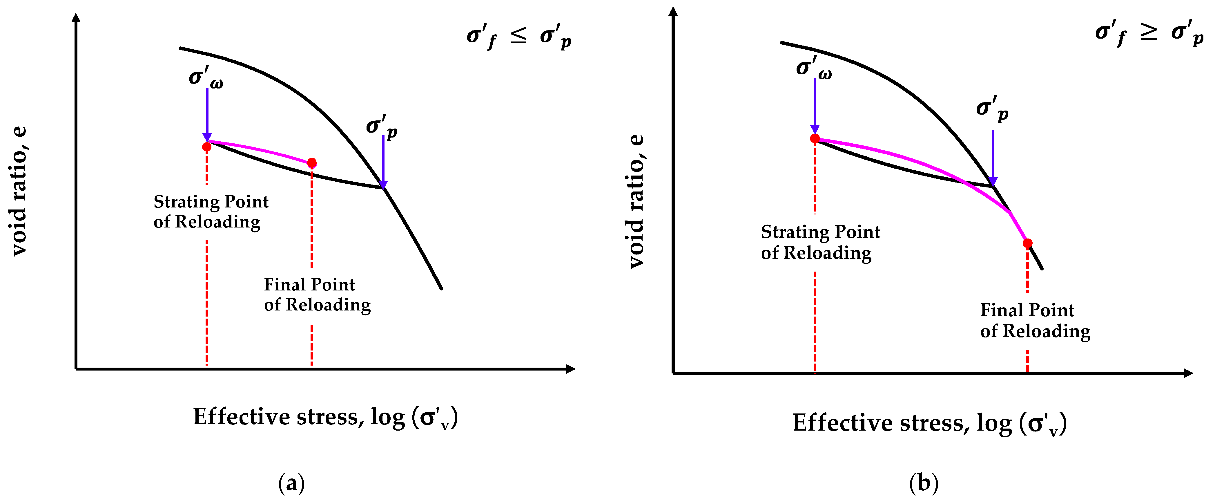
For the overconsolidated clay, it is necessary to calculate more steps as follows:

(6a)

Calculate the maximum past stress ${{\sigma }^{\prime }}_{p }=OCR·{{\sigma }^{\prime }}_{ini }$ which will be used as the unloading point ${{\sigma }^{\prime }}_{\mathcal{v}}$ on the VCL of each layer.

(6b)

Calculate the void ratio of the unloading point $e_{\vartheta new}$ at ${{\sigma }^{\prime }}_{p }$ in the step (6.1) using AJOP equation.

(6c)

Determine the parameters ($C^{\prime }$, $h^{\prime }$, and $k^{\prime }$) $=$ $f$($C$, $h$, and $k$) of the unloading of each midpoint.

(6d)

Calculate the void ratio of the initial stress $e_{int}$, which will be the same value of the void ratio of the starting point of reloading process $e_{\omega }$.

(6e)

Determine the parameters (${C_1}^{\prime }$, ${h_1}^{\prime }$, and ${k_1}^{\prime }$) $=f$($C$, $h,$ and $k$) of the reloading of each mid-point.

(7)

Calculate $\mathrm{\Delta }e$ between the initial and final stresses mentioned above in step (5) as follows:

(7a)

For NC (normally consolidated) clay, use Equation (7).

(7b)

For OC (overconsolidated) clay, use Equation (19) or (21).

(8)

Calculate the consolidation settlement of the $i^{th}$ layer using ${\rho }_i=H_i\left[{\displaystyle \frac{{\Delta e}_i}{1+e_0}}\right].$

(9)

The total consolidation settlement can be calculated as the sum of the settlements for each individual layer; i.e., $\rho =\sum _{i=1}^n\left({\rho }_i\right)$ when n is the number of soil layers.

4. Examples for the Prediction of One-Dimensional Consolidation Settlement

In this section, analytical computations are conducted using real soil parameters—three well-documented clays commonly referenced in geotechnical research, and applied to hypothetical loading and layering scenarios to evaluate the performance of the proposed method. To demonstrate the applicability and accuracy of the proposed equations, example calculations are performed to predict total consolidation settlement. A rectangular footing measuring 15 m × 30 m on a 12 m thick clay layer is used as the reference condition. Three virtual modeling scenarios were developed to examine the influence of different soil layering approaches on settlement prediction. The scenarios include:

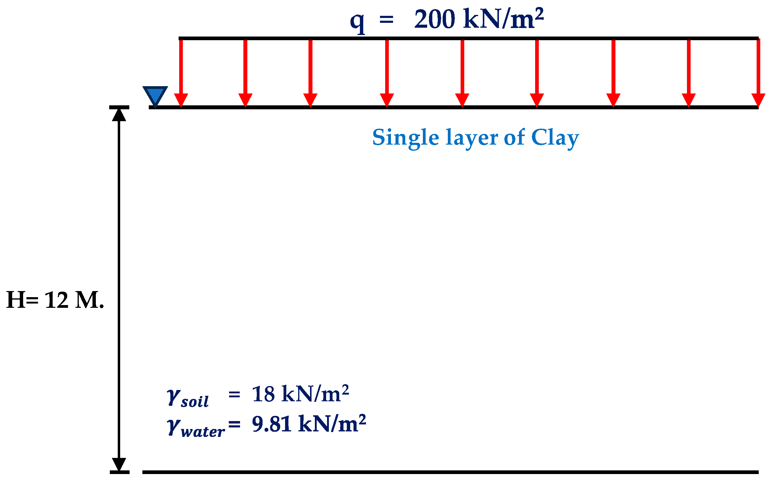
(a)

A single-layer clay model;

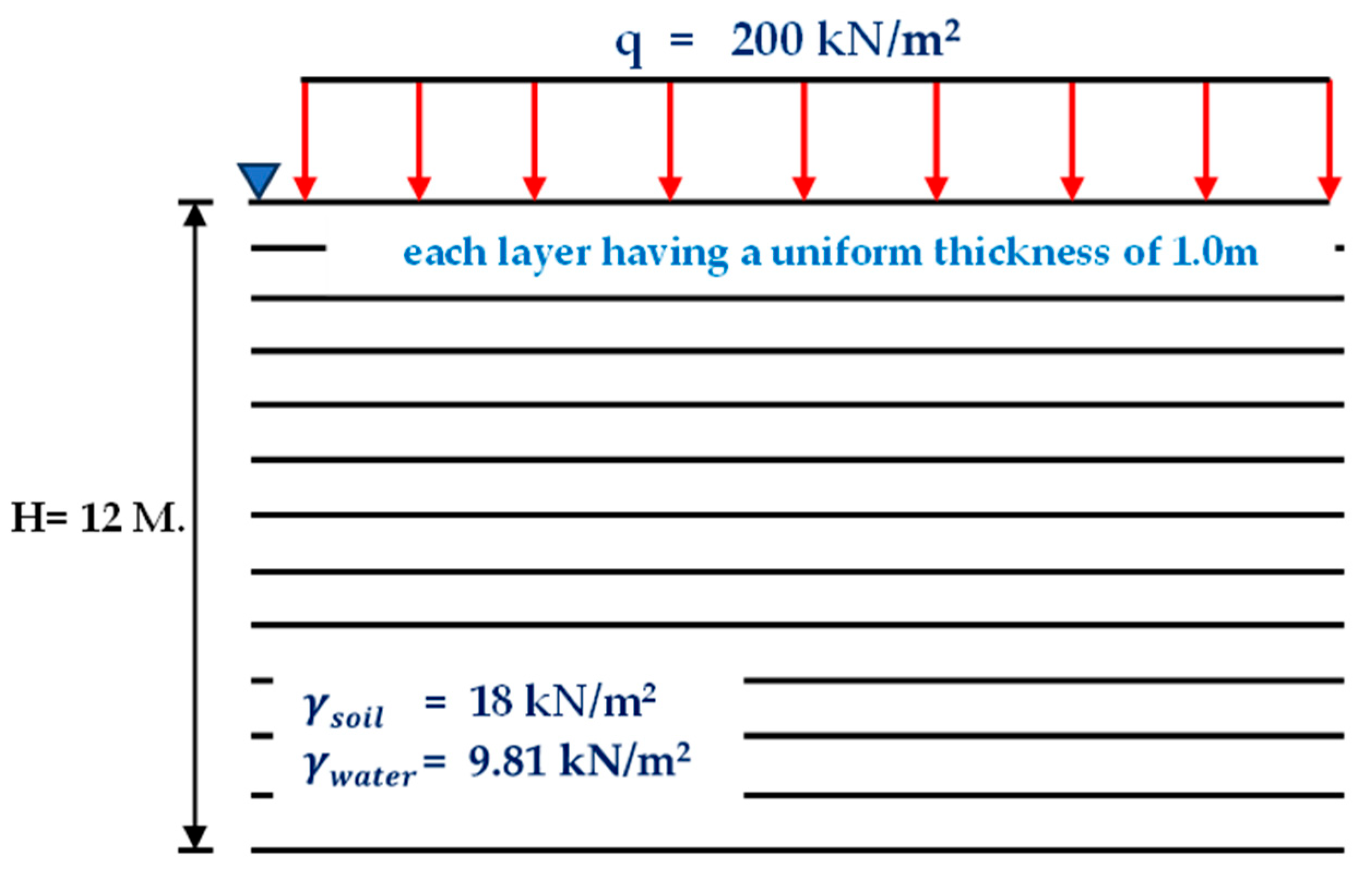
(b)

A multi-layer model with uniform layer thickness of 1 m;

(c)

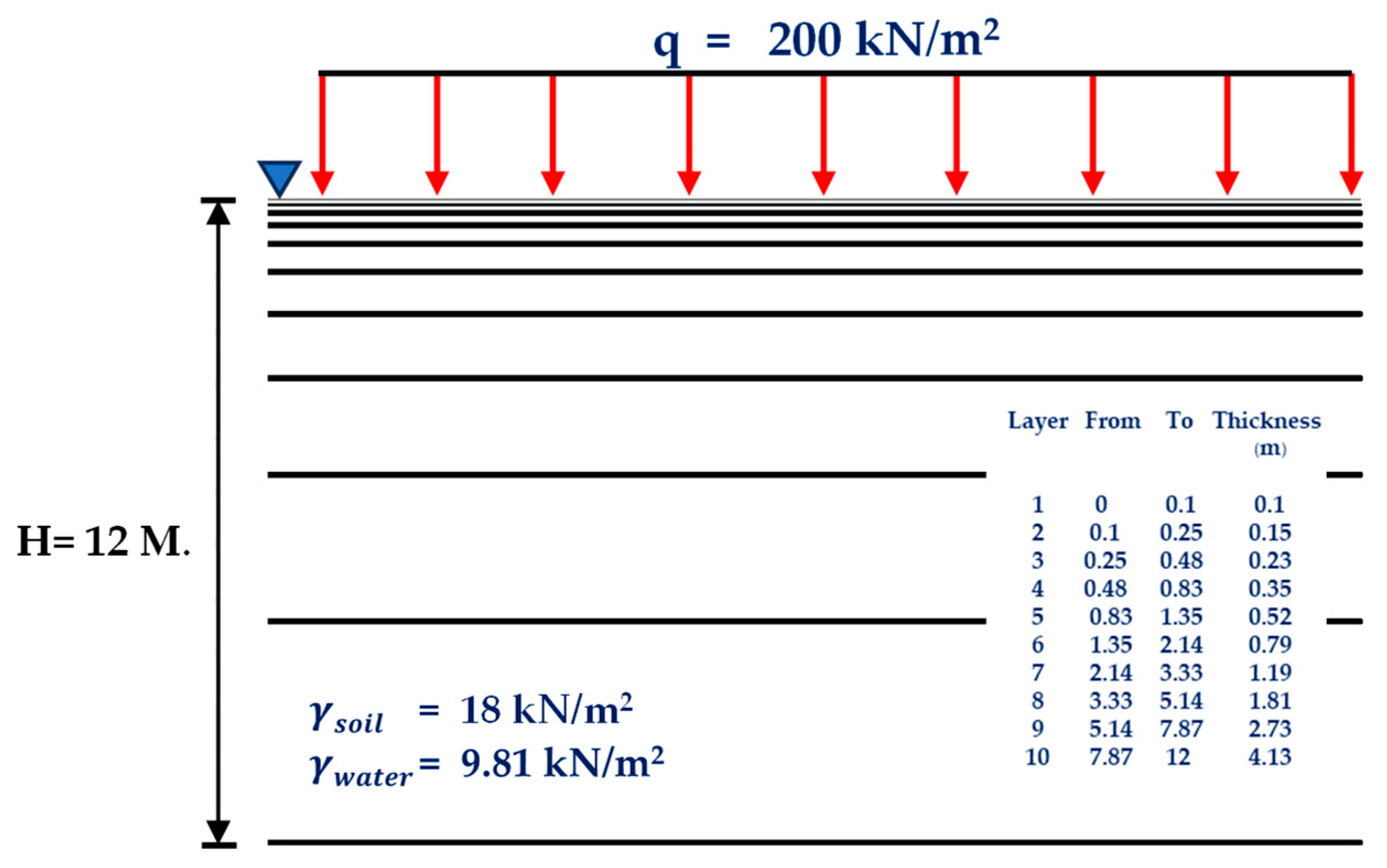
A variable-thickness layered model, in which thinner layers are used near the surface and layer thickness increases with depth.

It should be noted that the soil parameters employed in these examples were derived from previously published laboratory test results [22,23,24]. These well-documented clays provide a reliable basis for validating the proposed analytical model under controlled conditions. All soil parameters used in the tables and figures below are drawn from these established data sources and serve as reference inputs for the model evaluation.

Three soil test datasets from distinct continents were used for the consolidation test (i.e., Bangkok clay [22], Boston blue clay [23], and London clay [24]). Figure 6, Figure 7 and Figure 8 depict the test results from [22,23,24] with the best fit curves. Prior to the analysis, the soil parameters based on the proposed method were extracted.

Table 1. Soil parameters fitted from the laboratory test results.

Type of Soil	Virgin Compassion Line				Unloading–Reloading Line
	$\mathit{\Gamma }$	$\mathit{\alpha }$	$\mathit{R}$	$\mathit{\theta }$	$\mathit{C}$	$\mathit{h}$	$\mathit{k}$	$\mathit{\Psi }$
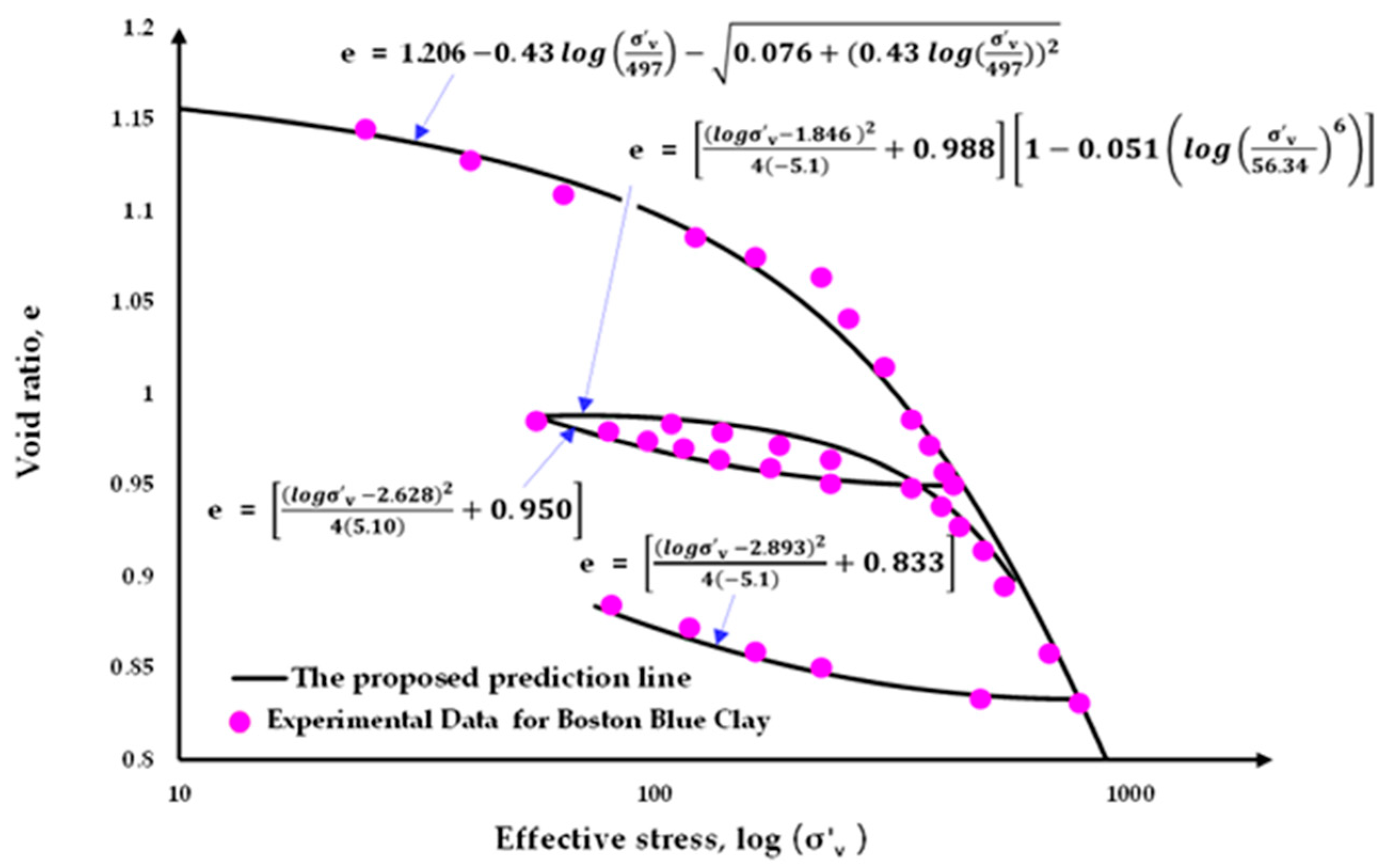
Boston blue clay	1.206	0.430	497	0.076	5.10	2.628	0.950	0.051
London clay	0.850	0.135	530	0.0058	5.70	3.800	0.64	0.004
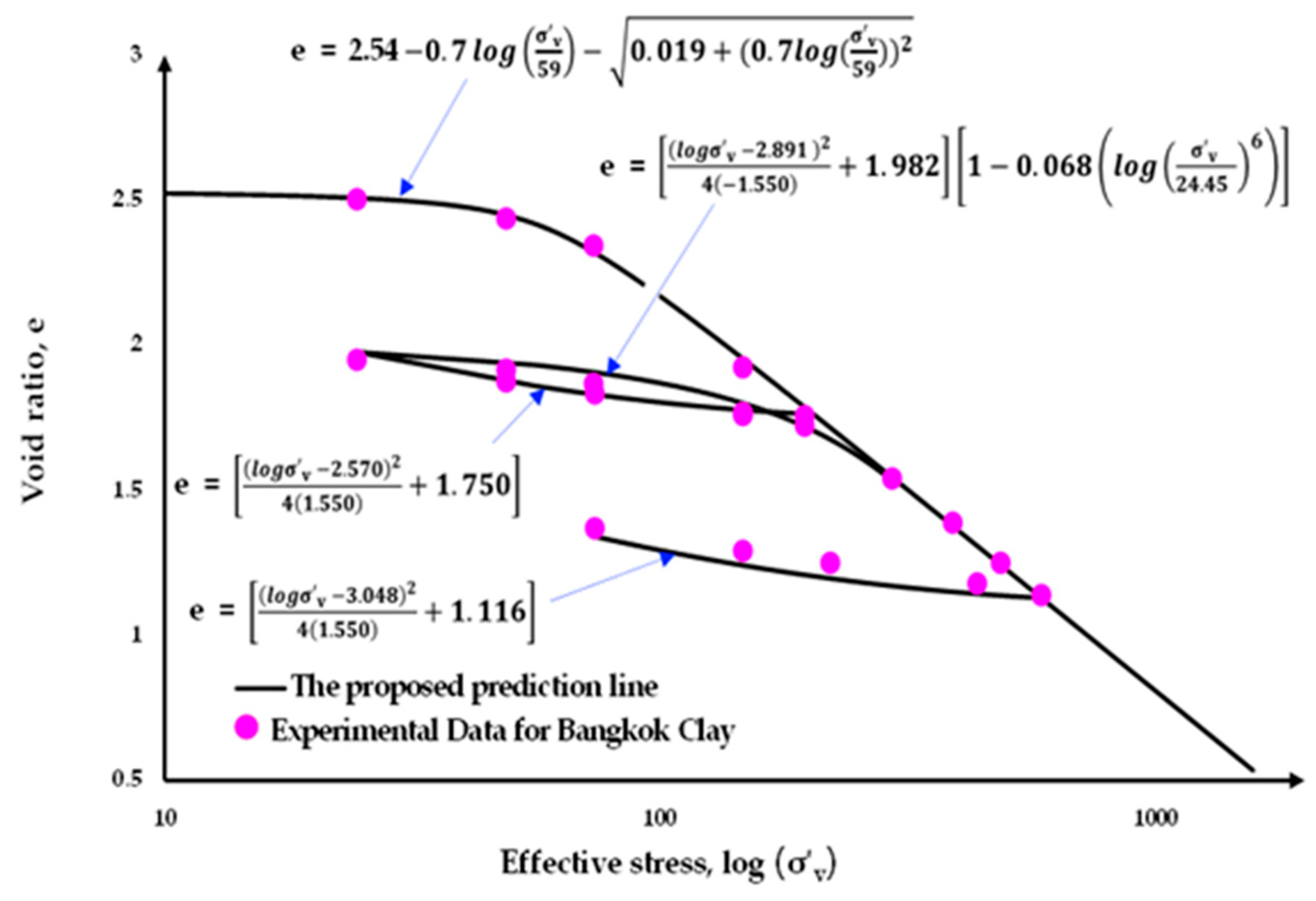
Bangkok clay	2.540	0.700	59	0.019	1.55	2.570	1.75	0.068

summarizes the fitting parameters for all three clays mentioned above. It should be noted that the soil parameters employed in these examples were derived from previously published laboratory test results [22,23,24]. These well-documented clays provide a reliable basis for validating the proposed analytical model under controlled conditions. The parameters $\Gamma , R, \alpha ,$ and $\theta$ are for the AJOP equation, and $C$, $h$, $k,$ and $\Psi$ are for the hysteresis portion. In the analysis of normally consolidated clay, three types of equations were applied, LF, CF, and AJOP. Figure 9, Figure 10 and Figure 11 show the problems to be analyzed for cases with a (a) single layer, (b) equal layer thickness, and (c) varied layer thickness, respectively. It should be noted that all clays behave with asymmetrical hysteresis ($\Psi \ne 0$).

Table 2. Comparison of total consolidation settlement of normally consolidated clay using LF, CF, and AJOP methods for three soil datasets.

Type of Soil	Case	LF (Equation (3))	CF (Equation (4))	AJOP (Equation (6))
Boston blue clay	(a) Single layer	1.566	0.302	0.284
	(b) Equal layer thickness	1.967	0.323	0.310
	(c) Varied layer thickness	1.988	0.323	0.309
London clay	(a) Single layer	0.806	0.102	0.089
	(b) Equal layer thickness	1.012	0.109	0.097
	(c) Varied layer thickness	1.023	0.108	0.097
Bangkok clay	(a) Single layer	2.334	3.453	1.832
	(b) Equal layer thickness	2.933	3.667	1.781
	(c) Varied layer thickness	2.964	3.663	1.780

shows the results of settlement calculations based on the aforementioned methods and conditions of the normally consolidated clay. It is evident that the settlement from the LF is much greater than that from the CF and AJOP because the actual initial stress on the shallow points is not located on the straight line of $e-log{{\sigma }^{\prime }}_v$. Therefore, the equations that provide the curved portion, i.e., CF and AJOP, give lower value and give more reliable results. It is also indicated in Table 2 that the results from CF and AJOP are close together, due to the impact of error on deeper depts being less than the impact at shallow depts. In addition, when the method of layer dividing is considered, the results using a single layer give the lowest value for all clays and all models. The results from the equal layer thickness model are close to the results for the method of varying layer thickness for all clays.

For the overconsolidated clay, the analyses were divided into two cases i.e., (1) low surface loading 200 kN/m², and (2) high surface loading 1000 kN/m².

Table 3. Comparison of total consolidation settlement for overconsolidated clay for low surface loading of 200 kN/m².

Type of Soil	Case	AJOP Method (Equation (6))
Boston blue clay	(a) Single layer	0.178
	(b) Equal layer thickness	0.207
	(c) Varied layer thickness	0.205
London clay	(a) Single layer	0.072
	(b) Equal layer thickness	0.080
	(c) Varied layer thickness	0.080
Bangkok clay	(a) Single layer	1.015
	(b) Equal layer thickness	1.119
	(c) Varied layer thickness	1.101

and

Table 4. Comparison of total consolidation settlement for overconsolidated clay for high surface loading of 1000 kN/m².

Type of Soil	Case	AJOP (Equation (6))
Boston blue clay	(a) Single layer	1.084
	(b) Equal layer thickness	1.139
	(c) Varied layer thickness	1.138
London clay	(a) Single layer	0.397
	(b) Equal layer thickness	0.417
	(c) Varied layer thickness	0.417
Bangkok clay	(a) Single layer	3.578
	(b) Equal layer thickness	3.659
	(c) Varied layer thickness	3.651

present the consolidation calculation results for overconsolidated clay in case (1) and case (2), respectively. In Table 3, the selected AJOP method is identified as the most reliable approach. The findings highlight the significant influence of the layer division method on the results. While using the AJOP equation, the single-layer division method yielded the lowest settlement due to the mid-layer being positioned farther from the ground surface. On the other hand, the multilayer division method provided more accurate results because the mid-points of some layers were closer to the ground surface, which is a critical factor for the AJOP method. In case (c), where layer thickness varies, the results were most accurate as the mid-points of the layers were correctly positioned. This demonstrates that both the calculation method and the layer division approach significantly affected the accuracy of the results. It should be noted that for this low surface loading value, we found that some soil layers were calculated with a final stress lower than the maximum past pressure.

Table 4 presents the calculation results under high loading conditions. In these calculations, both the compression ratio $\overline{C_r}$ and the compression index $\overline{C_{\mathrm{c}}}$ were used for Boston and Bangkok clays. However, for London clay, only the compression ratio $\overline{C_r}$ was utilized in the calculations in some depths. The findings show that although using different methods in layer division, the consolidation settlement was similar for all methods due to the fact that a single layer expressed the lowest value.

In both low-loading 200 and high-loading 1000 kN/m², it was revealed from the investigation that Case (1) (in Figure 5a) can occur but is not common at a specific depth, whereas Case (2) (in Figure 5b) generally occurs more frequently in both cases of low and high pressures.

5. Conclusions

The total amount of consolidation settlement in the field can be determined by the changes in void ratio based on the clay characteristics evaluated in the laboratory. This study focused on clays that creep, in which strain rate effects can be neglected, and especially clays exhibiting a curved portion followed by a straight portion in their $e-log{{\sigma }^{\prime }}_{\mathit{v}}$. We propose new equations that can fit well to the laboratory consolidation curve without any assumptions and additional testing. The proposed equations include (1) the revised version of the AJOP for normally consolidated clay, and (2) equation for both symmetrical and asymmetrical hysteresis of overconsolidated clay. With these equations, the analytical solution for consolidation settlement for clays can be established.

A comparison between the existing methods and the proposed method was investigated. The three methods of calculation were linear function (LF), curve function (CF), and the revised AJOP equation (function for curve and linear portions in a single equation). In addition, three models of clay layering were investigated, i.e., single layer, and multilayers with equal and varied thickness. Three clay datasets from different continents were used in the analysis, i.e., Bangkok clay, Boston blue clay and London clay.

For normally consolidated clay, it was revealed that the LF method yielded significantly higher consolidation settlement compared to the CF and AJOP methods for all clays and all layering conditions. Additionally, the single-layer model gave lower consolidation settlement than both layered soil models. These phenomena are influenced by two key factors: (1) the presence of curved portion in $e-log{{\sigma }^{\prime }}_{\mathit{v}}$, and (2) the omission and commission of the curved portion in calculations due to the soil layering method. Therefore, the CF method provided greater accuracy than the LF method because the curved portion exists in CF. However, the AJOP method reduced errors at both shallow and greater depths, as it incorporates both curved and linear segments within a single equation. For overconsolidated clay, only AJOP equation was selected in the analysis. The calculations yielded similar results across all models. However, all soil samples indicated that the non-layered soil model resulted in slightly lower settlement compared to the other two methods.

The findings highlight the significance of accurately modeling the void ratio and effective vertical stress relationship, particularly through a novel AJOP equation that combines curved and straight-line representation on a semi-logarithmic scale. This approach addresses the limitations of traditional methods, which often fail to capture the complexities of soil behavior at varying stress levels. Additionally, the authors have provided the recommendations in cases where sample disturbance and sensitive clay are encountered. The proposed method not only enhances the understanding of consolidation processes but also provides a practical tool for engineers in predicting settlement behavior more reliably. Future work may focus on refining the method and exploring its applicability to a broader range, such as the consolidation-creep framework and a constitutive model of clay.

References

- Davis, E.H.; Raymond, G.P. A Non-linear Theory of Consolidation. Geotechnique 1965, 15, 161–173. [Google Scholar] [CrossRef]
- Barden, L.; Berry, P.L. Consolidation of Normally Consolidated Clay. Soil Mech. Found. Div. 1965, 91, 5–35. [Google Scholar] [CrossRef]
- Gibson, R.E.; England, G.L.; Hussey, M.J.L. The Theory of One-Dimensional Consolidation of Saturated Clays. Geotechnique 1967, 17, 261–273. [Google Scholar] [CrossRef]
- Gray, H. Simultaneous consolidation of contiguous layers of unlike compressive soils. ASCE Trans. 1945, 110, 1327–1356. [Google Scholar]
- Poskitt, T.J. The Consolidation of Saturated Clay with Variable Permeability and Compressibility. Geotechnique 1969, 19, 234–252. [Google Scholar] [CrossRef]
- Schiffman, R.L.; Stein, J.R. One-Dimensional Consolidation of Layered Systems. Soil Mech. Found. 1970, 96, 1499–1504. [Google Scholar] [CrossRef]
- Mesri, G.; Rokhasar, A. Theory of Consolidation for Clays. Geotech. Eng. Div. 1974, 100, 889–904. [Google Scholar] [CrossRef]
- Lee, P.K.K.; Xie, K.H.; Cheung, Y.K. A Study on One-Dimensional Consolidation of Layered Systems. Int. J. Numer. Analyt. Methods Geomech. 1992, 16, 815–831. [Google Scholar] [CrossRef]
- Xie, K.; Pan, Q.Y. One-dimensional consolidation of soil stratum of arbitrary layers under time-dependent loading. China J. Geotech. Eng. 1995, 17, 82–87. [Google Scholar]
- Lekha, K.R.; Krishnaswamy, N.R.; Basak, P. Consolidation of Clays for Variable Permeability and Compressibility. J. Geotech. Geoenviron. Eng. 2003, 129, 1001–1009. [Google Scholar] [CrossRef]
- Zhuang, Y.C.; Xie, X.B.; Li, J. Nonlinear analysis of consolidation with variable compressibility and permeability. J. Zhejiang Univ. 2005, 6, 181–187. [Google Scholar] [CrossRef]
- Abbasi, N.; Rahimi, H.; Javadi, A.A.; Fakher, A. Finite Difference Approach for Consolidation with Variable Compressibility and permeability. Comput. Geotech. 2007, 34, 41–52. [Google Scholar] [CrossRef]
- Conte, E.; Troncone, A. Nonlinear Consolidation of thin layers Subjected to Time-Dependent Loading. Can. Geotech. 2007, 44, 717–725. [Google Scholar] [CrossRef]
- Carrera, E.; Brischetto, S. Analysis of Thickness locking in Classical, Refined and Mixed Multilayered Plate Theories. Compos. Struct. 2008, 82, 549–562. [Google Scholar] [CrossRef]
- Zheng, G.Y.; Li, P.; Zhao, C.Y. Analysis of Non-liner Consolidation of Soft Clay by Differential Quadrature Method. Appl. Clay Sci. 2013, 79, 2–7. [Google Scholar] [CrossRef]
- Li, C.; Huang, J.; Wu, L.; Lu, J.; Xia, C. Approximate Analytical Solutions for One-Dimensional Consolidation of a Clay Layer with Variable Compressibility and Permeability under a Ramp Loading. Int. J. Geomech. 2018, 18, 06018032. [Google Scholar] [CrossRef]
- Xie, K.H.; Xie, X.Y.; Jiang, W.A. Study on One-Dimensional Nonlinear Consolidation of Double-Layered Soil. Comput. Geotech. 2002, 29, 151–168. [Google Scholar] [CrossRef]
- Chen, R.P.; Zhou, W.H.; Wang, H.Z.; Chen, Y.M. One-Dimensional Nonlinear Consolidation of Multi-Layered Soil by Dif-ferential Quadrature Method. Comput. Geotech. 2005, 32, 358–369. [Google Scholar] [CrossRef]
- Hu, J.; Bian, X.; Chen, Y. Nonlinear Consolidation of Multilayer Soil under Cyclic loadings. Eur. J. Environ. Civ. Eng. 2021, 25, 1042–1064. [Google Scholar] [CrossRef]
- Kim, P.; Ri, K.S.; Kim, Y.G.; Sin, K.N.; Myong, H.B.; Paek, C.H. Nonlinear Consolidation Analysis of a Saturated Clay Layer with Variable Compressibility and Permeability under Various Cyclic Loadings. Int. J. Geomech. 2020, 20, 04020111. [Google Scholar] [CrossRef]
- Kim, P. Analytical Solution for One-Dimensional Nonlinear Consolidation of Saturated Multi-Layered Soil under Time-DePendent loading. J. Ocean Eng. Sci. 2021, 6, 21–29. [Google Scholar] [CrossRef]
- Trani, L.; Bergado, D.; Abuel-Naga, H. Thermo-Mechanical Behavior of Normally Consolidated Soft Bangkok Clay. Int. J. Geotech. Eng. 2010, 4, 31–44. [Google Scholar] [CrossRef]
- Whittle, A.J.; Degroot, D.J.; Seah, T.H.; Ladd, C.C. Model Prediction of The Anisotropic Behavior of Boston Blue Clay. J. Geotech. Eng. 1994, 120, 199–224. [Google Scholar] [CrossRef]
- Santos, L.M.; Oliveira, P.J.; Sousa, J.N.V.; Lemos, L.J.L. Effect of Initial Stiffness on The Induced Horizontal Displacements of Geotechnical Structures Built on/in Overconsolidated Clays. In Proceedings of the International Society for Soil Mechanics and Geotechnical Engineering, Imperial College, London, London, UK, 26–28 June 2023. [Google Scholar]
- Aysen, A. Soil Mechanics: Basic Concepts and Engineering Applications, 1st ed.; Swets & Zeitlinger, B.V.: Lisse, The Netherlands, 2002; pp. 221–222. [Google Scholar]
- Matsuoka, H.; Yao, Y.P.; Sun, D.A. The Cam-Clay Models Revised by the SMP Criterion. Soils Found. 1999, 39, 81–95. [Google Scholar] [CrossRef]
- Yao, Y.P.; Sun, D.A.; Luo, T.A. Critical State Model for Sands Dependent on Stress and Density. Int. J. Numer. Anal. Methods Geomech. 2004, 28, 323–337. [Google Scholar] [CrossRef]
- Yao, Y.P.; Sun, D.A.; Matsuoka, H. A Unified Constitutive Model for Both Clay and Sand with hardening Parameter Inde-pendent on Stress Path. Comput. Geotech. 2008, 15, 161–173. [Google Scholar]
- Cao, L.F.; Teh, C.I.; Chang, M.F. Undrained Cavity Expansion in Modified Cam Clay I: Theoretical Analysis. Geotechnique 2001, 51, 323–334. [Google Scholar] [CrossRef]
- Grimstad, G.; Degago, S.A.; Nordal, S. Modeling Creep and Rate Effects in Structured Anisotropic Soft Clays. Acta Geotech. 2010, 5, 69–81. [Google Scholar] [CrossRef]
- Yin, Z.Y.; Xu, Q.; Hicher, P.Y. A Simple Critical-State-Based Double-Yield-Surface Model for Clay Behavior under Complex loading. Acta Geotech. 2013, 8, 509–523. [Google Scholar] [CrossRef]
- Ou, C.Y.; Liu, C.C.; Chin, C.K. Anisotropic Viscoplastic Modeling of Rate-Dependent Behavior of Clay. Int. J. Numer. Anal. Methods Geomech. 2011, 35, 1189–1206. [Google Scholar] [CrossRef]
- Li, X.S.; Wang, Y. Linear Representation of Steady State Line for Sand. J. Geotech. Geoenviron. Eng. 1998, 124, 1215–1217. [Google Scholar] [CrossRef]
- Yang, Z.X.; Li, X.S.; Yang, J. Quantifying and Modelling Fabric Anisotropy of Granular soils. Geotechnique 2008, 58, 237–248. [Google Scholar] [CrossRef]
- Yang, J.; Wei, L.M.; Dai, B.B. State Variables for Silty Sands: Global Void Ratio or Skeleton Void Ratio? Soils Found. 2015, 55, 99–111. [Google Scholar] [CrossRef]
- Murthy, T.G.; Loukidis, D.; Carraro, J.A.H.; Prezzi, M.; Salgado, R. Undrained Monotonic Response of Clean and Silty Sands. Geotechnique 2007, 57, 273–288. [Google Scholar] [CrossRef]
- Rahman, M.M.; Lo, S.R.; Baki, M.A.L. Equivalent Granular State Parameter and Undrained Behaviour of Sand–Fines Mixtures. Acta Geotech. 2011, 6, 183–194. [Google Scholar] [CrossRef]
- Rahman, M.M.; Lo, S.R.; Dafalias, Y.F. Modelling the Static Liquefaction of Sand with Low-Plasticity Fines. Geotechnique 2014, 64, 881–894. [Google Scholar] [CrossRef]
- Duriez, J.; Vincens, É. Constitutive Modelling of Cohesionless Soils and Interfaces with Various Internal States: An Elas-to-Plastic Approach. Comput. Geotech. 2015, 63, 33–45. [Google Scholar] [CrossRef]
- Kaewhanam, N.; Chaimoon, K. A Simplified Silty Sand Model. Appl. Sci. 2023, 13, 8241. [Google Scholar] [CrossRef]
- Yin, J.H.; Graham, J. General Elastic Viscous Plastic Constitutive Relationships for 1-D Straining in Clays. Int. Symp. Numer. Models Geomech. 1989, 3, 108–117. [Google Scholar]
- Yin, J.H.; Graham, J. Equivalent Times and One-Dimensional elastic Viscoplastic Modelling of Time-Dependent Stress–Strain Behaviour of Clays. Can. Geotech. J. 1994, 31, 42–52. [Google Scholar] [CrossRef]
- Yin, J.H.; Graham, J. Elastic Visco-Plastic Modelling of One-Dimensional Consolidation. Geotechnique 1996, 46, 515–527. [Google Scholar] [CrossRef]
- Yin, J.H. Non-Linear Creep of Soils in Oedometer Tests. Geotechnique 1999, 49, 699–707. [Google Scholar] [CrossRef]
- Zhu, Q.-Y.; Yin, Z.-Y.; Hicher, P.-Y.; Shen, S.-L. Nonlinearity of One-Dimensional Creep Characteristics of Soft Clays. Acta Geotech. 2016, 11, 887–900. [Google Scholar] [CrossRef]
- Nishimura, T. Shear Strength of an Unsaturated Silty Soil Subjected to Creep Deformation. Geotech. Sustain. Infrastruct. Dev. 2020, 62, 977–984. [Google Scholar]
- Degago, S.A.; Nordal, S.; Grimstad, G.; Jostad, H.P. Analyses of Väsby Test Fill according to Creep Hypothesis A and B. In Proceedings of the International Conference of the International Association for Computer Methods and Advances in Geomechanics, Melbourne, Australia, 9–13 May 2011. [Google Scholar]
- Leroueil, S.; Kabbaj, M.; Tavenas, F.; Bouchard, R. Stress–Strain–Strain Rate Relation for the Compressibility of Sensitive Natural Clays. Géotechnique 1985, 35, 159–180. [Google Scholar] [CrossRef]