Algorithm for Determining the Position of a Ship Hull-Cleaning Robot

Abstract

The paper explores the development and evaluation of algorithms for the positioning of ship hull cleaning robots, focusing on machine learning and sensor fusion techniques. The research employs Gradient Boosting, Kalman filters, and deep learning to enhance the accuracy of robot positioning. Gradient Boosting is used to predict displacement vectors and rotation angles, while the Kalman filter is applied to refine position estimates by integrating odometry and GPS data. Deep learning models are utilized to predict robot trajectories based on sensor inputs. Experiments conducted on the Rosario dataset and simulated environments demonstrate the effectiveness of these methods.

1. Introduction

The accurate positioning and navigation of autonomous robots operating on ship hull surfaces is a critical challenge in maritime robotics. Regular cleaning of the ship hulls is essential to maintain vessel efficiency, reduce fuel consumption, and minimize environmental impact by preventing biofouling. Traditionally, hull cleaning operations require ships to be docked or dry-docked, resulting in downtime and increased operational costs. Autonomous hull cleaning robots offer a promising alternative, enabling efficient and continuous maintenance without the need to remove vessels from the water. However, the effectiveness of these robots is highly dependent on their ability to precisely determine their position and orientation on the hull surface, especially in challenging underwater environments.

However, although positioning is widely recognized as an important factor for hull cleaning robots, most prior work focuses primarily on the design and construction of robots tailored to specific cleaning tasks or hull environments, rather than on the development of positioning algorithms. Many studies present robots with unique mechanical architectures or cleaning mechanisms, such as morphologically intelligent underactuated robots for non-magnetic hulls [1], hydroblasting reconfigurable robots [2], or systems equipped with hydraulic manipulator arms for cleaning niche areas [3]. In these works, the positioning subsystem is often closely coupled to the specific hardware and operational context of the robot.

When positioning is addressed, it is frequently realized through specialized sensor suites or infrastructure-dependent methods. Some robots rely on vision-based simultaneous localization and mapping (SLAM) algorithms using cameras [4], or on the fusion of laser scanners and 3D CAD models [3], which require visual data and prior models of the hull. Others employ optical dead-reckoning systems based on mouse sensors [5,6], or magnetic landmark recognition systems that depend on the internal structure of the hull. Advanced approaches integrate Doppler velocity logs, imaging sonars, and monocular cameras within SLAM frameworks [7], or utilize networks of ultrasonic beacons for 3D location [2]. Although these methods can achieve high accuracy, they often require additional infrastructure (e.g., beacons, reference landmarks), complex sensor fusion, or are limited to specific operational scenarios.

This paper focuses specifically on the development and evaluation of a general-purpose positioning algorithm for ship hull cleaning robots, independent of the robot’s mechanical design or the need for external infrastructure. Our approach combines classical kinematic computations with advanced sensor data processing techniques. By integrating odometry and inertial measurement unit (IMU) data, enhanced with state-of-the-art methods such as Kalman filtering, our work aims to improve the accuracy and reliability of the robot’s navigation along the side of the ship. Our system detects and corrects the effects of wheel slippage, a common source of error in odometry-based positioning, by correlating encoder readings with observed orientation changes from IMU sensors. Unlike prior works that require additional sensors (e.g., Lidar, sonar, beacons) or hull modifications (e.g., magnetic landmarks), our method is designed to operate with a minimal sensor set—wheel encoders and an IMU. To evaluate our approach, we developed an experimental framework tested on publicly available datasets and simulated data modeling real-world scenarios, including artificial slip events.The real-world scenarios were prepared in collaboration with SR Robotics (https://srrobotics.pl/), a company specializing in the design and construction of remotely operated and autonomous underwater and surface robots that support operations in marine and inland water environments.

The contributions of this paper are as follows. First, we present a positioning algorithm that integrates kinematic models with corrective techniques based on machine learning and probabilistic filtering. Second, we demonstrate how deep learning architectures can predict corrective displacements by leveraging temporal patterns in sensor data, thereby mitigating the cumulative error typically associated with odometry. Finally, our extensive experimental evaluations provide insight into the performance trade-offs between different correction frequencies and sensor fusion strategies, forming the optimal integration of these methods in real-world hull-cleaning applications.

In the following sections, we survey related work on hull-cleaning robot positioning, detail the methodologies adopted, including machine learning algorithms, Kalman filters, and deep learning approaches, and present our experimental setup and results.

2. Research Context

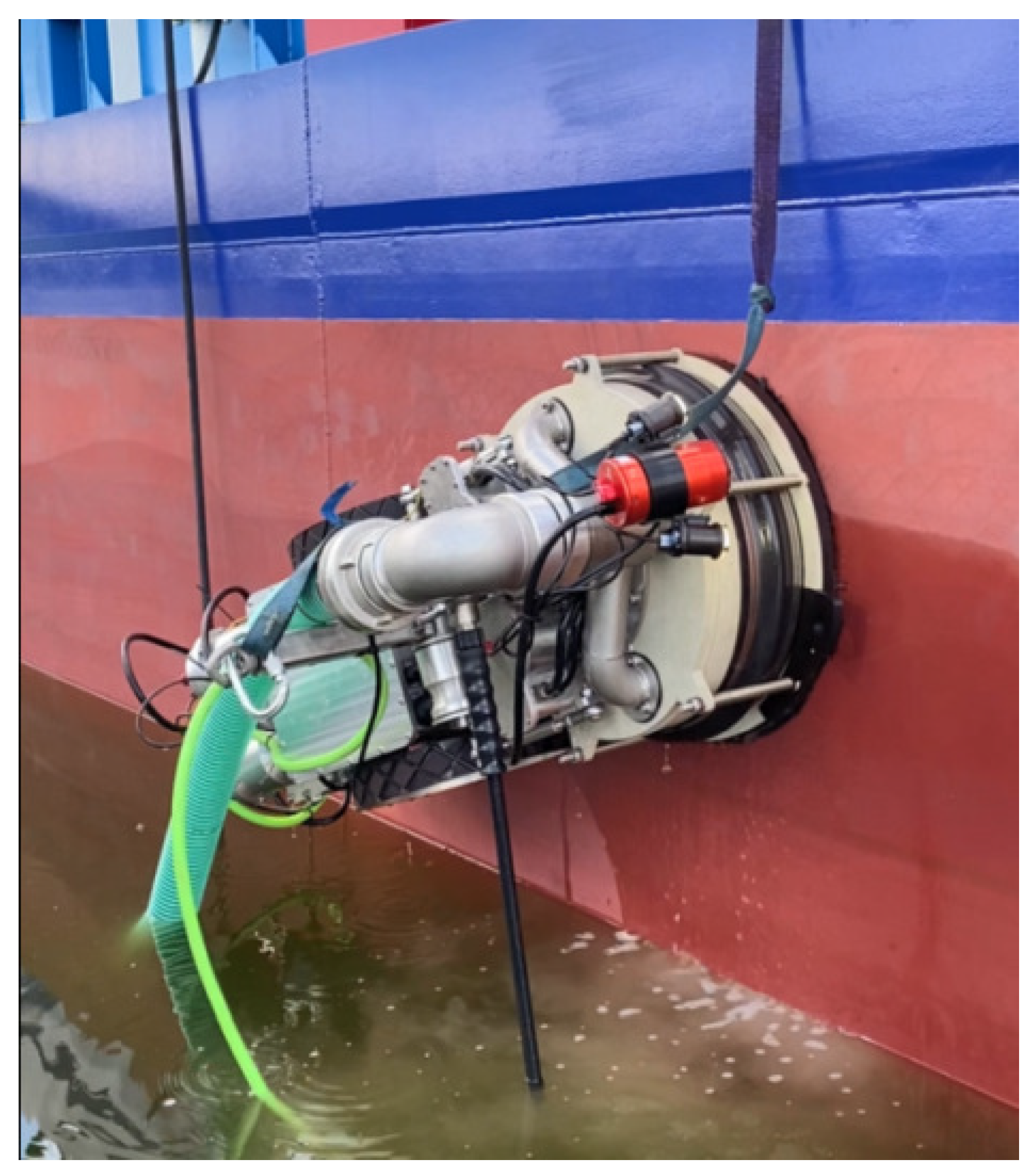
The development of SR Robotics’ magnetic adhesion robot marks a significant advancement in the domain of autonomous maintenance systems for marine and industrial infrastructure. Designed to operate on ferromagnetic surfaces both above and below the waterline, the robot offers a comprehensive solution for cleaning ship hulls and, additionally, surfaces such as petrochemical tanks, without requiring the vessel or structure to be decommissioned or dry-docked. Its ability to navigate and perform cleaning operations throughout the full surface of the hull, while continuously extracting contaminants and documenting the process via video cameras onboard, represents a unique integration of mechanical, environmental, and digital functionalities.

As part of a recent R&D initiative, SR Robotics developed this innovative robotic system (Figure 1) to address critical challenges related to biofouling and corrosion, significantly improving the efficiency, quality, and safety of surface maintenance operations. Operating with a water pressure of up to 2500 bar and sufficient magnetic adhesion forces to move reliably on vertical metallic structures, the robot is equipped with a specialized cleaning module, a high-efficiency waste extraction system (approximately 95%), advanced localization sensors, optical inspection cameras, and data acquisition tools compliant with Industry 4.0 standards. It is remotely controlled via an umbilical cable or a radio link, enabling safe and flexible deployment in various working environments.

A key challenge in the development of this system was the need for a universal positioning algorithm capable of supporting navigation in both submerged and above-water environments. Conventional navigation methods such as GPS are limited to surface operations, while hydroacoustic positioning systems or Doppler Velocity Logs (DVL) function only underwater. SR Robotics and its research partners addressed this challenge by developing a positioning system based on odometry and inertial measurement units (IMUs), which operate effectively in both domains. This foundational approach provides reliable relative positioning while allowing for modular enhancements. In underwater scenarios, additional sensors, such as DVLs and depth sensors, can be integrated; conversely, GPS receivers can be utilized for surface-level operations. This hybrid architecture ensures flexibility, scalability, and robustness of the navigation solution.

The requirement for a new positioning algorithm was driven by the robot’s unique mission profile—full-hull coverage across variable environments—where existing solutions lacked the adaptability and precision required for seamless transitions between above-water and submerged navigation. As a result, the algorithm described in this article forms a critical component of a system that not only automates hull maintenance but also sets new standards for operational autonomy and environmental compliance in the maritime and industrial sectors.

3. Related Works

Recent advances in hull-cleaning robot positioning have leveraged a variety of sensor technologies and intelligent algorithms to improve navigation and operational efficiency in challenging environments.

The article [8] presents a preliminary design of an underwater robotic complex designed for the inspection and laser cleaning of ship hulls from biofouling. In the context of robot navigation, the paper states that the navigation data for planning the vehicle’s trajectory are obtained from a combination of wheel odometry and visual odometry. To achieve navigation accuracy, the proposed complex utilizes the following equipment:

• A standard set of navigation equipment (vehicle depth, pitch, roll, yaw, and angular velocities).
• A long-baseline hydroacoustic navigation system with one or two beacon repeaters.
• A wheel-based odometry system.
• A visual odometry system based on photo data from an on-board camera.

The combination of these different methods is intended to increase the navigation accuracy of the underwater vehicle when inspecting and cleaning ship hulls. It is important to note that the research outlines a preliminary design of the cleaning robotic complex.

Another example in which visual odometry has been employed is [9]. The paper proposes an autonomous ship hull inspection strategy using an Autonomous Underwater Vehicle (AUV) equipped with a stereo camera and a proximity sensor. The AUV localizes itself relative to the hull without prior knowledge of its shape. Stereo vision is used to estimate the AUV’s lateral velocity and orientation relative to the hull. These orientation data are fused with IMU angular velocity measurements using an Extended Kalman Filter (EKF) called the Relative Orientation Filter (ROF) to improve accuracy. The proximity sensor provides distance measurements, which are projected along the normal axis to the hull. Stereo Visual Odometry (SVO) estimates the lateral velocity, and these data are fused with IMU and depth sensor data. This estimated lateral velocity is used for the AUV’s control. In summary, the robot is localized by combining stereo vision (for orientation and lateral velocity), a proximity sensor (for distance), and IMU (for angular velocity).

In [4], a system enabling an Autonomous Underwater Vehicle (AUV) to perform long-term ship hull inspections using SLAM was described. A key challenge addressed is achieving accurate localization relative to the ship hull without relying on acoustic beacons. The system utilizes a Doppler Velocity Log (DVL) as a primary navigation sensor, operating in hull relative or seafloor relative mode. It also incorporates visual SLAM using underwater and periscope cameras to derive spatial constraints. A significant contribution is the representation of the ship hull as a collection of locally planar surface features, which are integrated into the SLAM framework. The system prioritizes the relative navigation of the hull, as the position of the ship in a port can change with time, making absolute navigation methods less suitable.

The article [1] discusses a new type of robot designed to clean underwater ship hulls, especially those with non-magnetic hulls. The aim of the project was to improve the efficiency of ships by regularly cleaning their hulls without having to take them out of the water. The robot is designed as a morphologically adapted robot, which means that its structure and operation are adapted to harsh conditions under water.

The key element is an advanced positioning system that allows the robot to move independently on the surface of the hull. The robot is equipped with a set of sensors that collect the necessary data to determine its position and orientation. The technologies used include the following:

• Inertial measurement unit (IMU)—provides information about the robot’s orientation in space,
• Absolute pressure sensor—measures the depth at which the robot operates,
• Encoders—each of the robot’s moving joints is equipped with encoders that track the angle of rotation of individual parts.

The robot also uses a sensor system to monitor its condition and its surroundings. Differential pressure sensors measure the pressure inside the suction chamber, allowing it to determine whether the module is attached to the hull surface. In addition, a set of sonar sensors placed around the modules allow for obstacle detection and collision avoidance.

Robot control is based on a hierarchical system that consists of three levels. The highest level calculates the route the robot should follow, while the middle level is responsible for reactions to obstacles and maneuvers based on information from the sensors. The lowest level controls motors and devices.

In [2], the architecture of the Hornbill robot is described, which was used to autonomously clean the surface of ships by hydroblasting. The robot operates in manual and autonomous modes, which allows the operator to adjust the method of operation depending on the situation. To determine the robot’s position on the ship’s surface, an ultrasonic-based beacon system is used, where a mobile beacon on the robot calculates its relative 3D position within a network of stationary beacons by sensing ultrasonic waves. The system uses advanced signal processing from various sensors. The input data includes data from the wheel encoders, as well as the orientation provided by the IMU sensor. This data is then processed by a Kalman filter to eliminate noise and obtain a precise robot location. The Hornbill robot is equipped also with a camera used to record video to classify the cleanliness of the surface after cleaning and an IMU responsible for determining the robot’s orientation on a vertical surface. Using sensors, the robot generates position data in the form of ROS 3D messages, which contain information about the robot’s position in the 3D system. Thanks to the sensor fusion algorithm, it is possible to eliminate noise from the measurement data and obtain more reliable information about the robot’s position.

The article [6] focuses specifically on the development of a localization system for underwater hull-cleaning robots. The authors present a solution based on optical technology, not using cameras or Lidar in the traditional sense, but rather a customized optical mouse sensor system adapted for underwater use. The primary localization technology discussed is an optical position sensor (OPS), which uses a laser optical mouse sensor combined with a telecentric lens to achieve dead-reckoning navigation on the hull surface. In addition to the OPS, the system integrates data from a landmark recognition sensor (LRS) that uses magnetic flux leakage to detect features such as welds. The OPS provides relative position information between these known features, supporting semi-autonomous or autonomous operation. In summary, the article presents a localization system for a ship hull crawling robot that uses an optical tracking system for continuous relative positioning and a LRS for detecting fixed landmarks.

In [3], the development of an autonomous cleaning robot equipped with a hydraulic manipulator arm is presented. The robot utilizes a laser scanner to map the cleaning area and employs path planning algorithms and dynamic simulation to optimize the arm’s movements and avoid collisions. The primary localization technology used in the article is an underwater laser scanner mounted on the fifth link of the robot’s hydraulic arm. This scanner generates point cloud data on the cleaning area by moving in a lawnmower pattern. The obtained point cloud data are then matched with an existing precise 3D CAD model of the niche area using the Iterative Closest Point (ICP) algorithm to estimate the relative location and positioning between the robot and the target cleaning zone. Furthermore, a multi-beam echo sounder is installed in the robot body to recognize the surrounding topography and provide an approximate location of the niche area.

The article [5] discusses the significant problem of biological buildup in ship hulls, which leads to increased drag, fuel consumption, corrosion, and biological pollution. The article indicates that the HISMAR robot employs a new navigation system to achieve autonomous operation. This system utilizes a combination of sensors and software for localization and mapping. Specifically, it includes an optical dead reckoning system (ODRS), which uses optical mouse sensors to measure displacement and reduce the impact of wheel slippage. Additionally, a magnetic landmark recognition system (MLRS) is used to detect the internal structure of the ship’s hull, providing data for mapping and navigation. The data from the ODRS and MLRS are used by the software to create a magnetic landmark map of the ship’s hull. This map is then used to plan the robot’s working trajectory.

Article [7] discusses advanced perception, navigation, and planning methods for Autonomous Underwater Vehicles (AUVs), conducting inspections of the hulls of ships. It addresses challenges posed by the underwater environment and complex structures, presenting sonar- and vision-based SLAM algorithms and path planning for comprehensive surface coverage. The Hovering Autonomous Underwater Vehicle (HAUV) utilizes several localization technologies. For basic navigation, it employs a Doppler velocity log (DVL) locked to the hull or seafloor, an inertial measurement unit (IMU) for attitude, and a depth sensor. More advanced drift-free localization is achieved through Simultaneous Localization and Mapping (SLAM). This SLAM system integrates data from an imaging sonar and a monocular camera to build a map and simultaneously localize the vehicle.

In addition to the methodological approaches discussed earlier, several datasets with similar characteristics were identified in the literature. In the following, we briefly describe a selection of them, highlighting their relevance and limitations in the context of our research. The CoreNav-GP dataset [10] contains GPS and IMU data collected in various environments, similar in scope to the types considered in this research. However, it turned out to be inappropriate for our purposes. Attempts to unpack the files using Python scripts often resulted in unexpected end-of-file errors, and the dataset appears to lack a reference position (ground truth). For these reasons, CoreNav-GP was excluded from further consideration. The KITTI dataset [11] is a well-known benchmark that provides a variety of sensory data for autonomous driving, including GPS and stereo vision, and was initially considered. However, it lacks inertial measurements (IMU) and wheel encoder data, which are essential for the evaluation of the methods considered in this study. As a result, it was not used in our experiments. The last of the datasets found was the Rosario dataset [12], which turned out to be the most relevant to our research. It included the sensor data required for our project and featured a movement pattern analogous to the expected motion of the robot along the hull of the ship.

4. Methods

In our experiments, we focused on three approaches for data analyzing and processing: Gradient Boosting, Kalman filter and deep learning. The selection of them came from other studies that had applied these methods for comparable issues: [13,14] (Gradient Boosting), [15,16] (Kalman filter), and [14,17,18] (deep learning).

4.1. Machine Learning Approach

Gradient Boosting is a type of ensemble-supervised machine learning algorithm that improves the accuracy of predictive models by combining multiple simpler base models (“weak learners”, for example, decision trees) into a stronger ensemble [19]. The process is iterative, and the subsequently added learners are specifically trained to correct the errors made by the previous models. These errors are identified by large residuals computed in the previous iterations. Instead of predicting the actual target value, each new learner focuses on predicting the residuals. Therefore, the direction of improvement is determined by the negative gradients of the loss function, which indicates how the ensemble should be adjusted to minimize errors [20,21].

In practical applications, Gradient Boosting can be adapted to various types of data and to regression and classification problems. An arbitrary selection of the base model and the loss function make Gradient Boosting a very flexible and versatile method that can be adjusted to a specific type of problem. For example, popular Gradient Boosting frameworks such as CatBoost, XGBoost, and LightGBM have been successfully applied in various industries, e.g., finance [22], healthcare [23], energy storage systems [24].

4.2. Kalman Filter

The Kalman filter is a method developed by Rudolf Kalman and Richard Bucy in the 1960s to estimate the value of an observed variable based on its previous values and assuming that they may be subject to error [25]. The model consists of three matrices (input, state, and output), as well as two quantities denoting process and measurement noise, respectively.

In the case of discrete process modeling, the use of the Kalman filter consists of two phases: the first involves taking into account the passage of time (making a prediction of the forecasted variable as well as updating the covariance between the forecasted and actual values), while the second concerns updating the values of the remaining matrices constituting the model.

Due to its smoothing and auto-tuning properties, the Kalman filter is used in many fields related to measurements, including in issues related to determining the position of devices in space or on a plane [26,27,28].

4.3. Deep Learning

Deep learning is a subfield of machine learning that focuses on using neural networks with multiple layers to model complex patterns in data. Recurrent Neural Networks (RNNs) are a specific type of neural network used within deep learning, particularly suited for handling sequential data. By maintaining an internal state that encodes the setting of previous input data, RNNs can be used when temporal relationships within the data are important [29]. However, despite their advantages, RNNs usually cannot handle long-term dependencies due to problems like vanishing and exploding gradients. As the sequences are longer, the RNNs can lose important information presented earlier in the input, which limits their performance in deeper sequence contexts [30].

Starting from [31], many theoretical and experimental studies have been conducted on the Long Short-Term Memory (LSTM) network in order to address the limitations of RNNs. LSTM architecture is specifically designed to learn long-term dependencies in sequence data [32]. It consists of the memory cell, input gate, forget gate, and output gate, which work together, selectively maintain, or discard information. This approach to control how much of the past information should be forgotten improves the performance of predictions with respect to the broader context of the data [33]. Due to their properties, LSTMs have been successfully applied to solve problems in Natural Language Processing [33], finance [34], healthcare [35], or in navigation in complex and dynamic environments [36,37,38].

5. Data Sets

In the available literature, one can find many datasets concerning the issue of SLAM (Simultaneous Localization and Mapping), collected in cities, inside buildings, and also in difficult, diverse terrain (e.g., on unpaved ground, in fields, underwater). Unfortunately, most of them did not provide a minimal set of sensors from the point of view of the research problem (i.e., data from GPS, IMU, and odometry), or the recorded routes were not complicated (e.g., the data contained only straight-line travel). Hence, the selection of popular data is defined as Rosario [39]. Experiments carried out with different methods on this dataset resulted in a new algorithm to determine the position of a moving object (Section 5.1).

Ultimately, the algorithm mentioned above was to be used to determine the position of an object moving along the ship’s side. Hence, it was necessary to provide reference data that describe the behavior of the sensors and their readings during sample runs. These experiments are described in Section 5.2.

Since one of the critical phenomena affecting the accuracy of determining the device’s position turned out to be the so-called slippages, further tuning of the model was carried out using a simulator. Its task was to generate signal waveforms for the assumed route of the device, along with the possibility of artificially introducing moments of the slippages mentioned above. The description of these data is included in Section 5.3.

5.1. Rosario Dataset

Before developing the project-related data and models, we decided to test the above-mentioned methods on some benchmark dataset, and the Rosario dataset [12] became our choice.

The Rosario dataset was collected using a mobile robot (Figure 2) designed for outdoor agricultural environments [12]. The robot was equipped with a TARA stereo-inertial sensor (LSM6DS0 IMU), operating at a frequency of 140 Hz. For global localization, the system includes a GPS-RTK Emlid Reach module, operating at a frequency of 5 Hz. A ZED stereo camera was also mounted on the robot to collect synchronized left and right images at a resolution of 672 × 376 px and at a frame rate of 15 Hz.

Data were recorded on the open grounds of the Universidad Nacional de Rosario (Argentina), specifically in a grassy field used for testing mobile robotics in agricultural-like outdoor environments. The ROSARIO dataset consists of six recorded routes of varying difficulty collected by the robot in soybean fields. The dataset contains synchronized readings from the following sensors (the measurement frequency is given in brackets):

• odometry (10 Hz);
• IMU (140 Hz);
• GPS (5 Hz);
• stereo cameras (this information was not used in the experiments).

In particular, the information provided by each sensor is as follows:

• from the odometry sensor:

  −

  time stamp,

  −

  calculated position of the robot in the XYZ coordinate system,

  −

  linear velocity,

  −

  angular velocity.

• from the IMU sensor:

  −

  time stamp,

  −

  orientation of the robot in free space in the form of quaternions,

  −

  angular velocity,

  −

  linear acceleration.

• from the GPS-RTK system:

  −

  time stamp,

  −

  latitude,

  −

  longitude,

  −

  altitude,

  −

  linear velocity,

  −

  angular velocity

  −

  position covariance defined with respect to the tangent plane.

In this work, we assume the GPS-RTK position as ground truth, as the system used (GPS-RTK Emlid Reach) has been shown to achieve centimeter-level accuracy. The precision of this GPS-RTK configuration has been evaluated in [40], where the mean positioning error in Fix mode (the state in RTK-GPS positioning where the receiver has successfully resolved carrier phase ambiguities) was reported to be around 5 mm with a sampling rate of 5 Hz.

As mentioned, the data include six runs with a total length of 2296.93 m, completed in 34.7 min. The first run was in the north–south direction, while the rest, according to the suggested robot movement pattern, was in the east–west direction. The summary of the length and duration of each run is presented in

Table 1. Summary of the distance and duration of each of the analyzed sequences.

Sequence	Length [m]	Duration [s]
1	615.15	558
2	320.16	264
3	169.45	198
4	152.32	162
5	330.43	312
6	709.42	588

. The actual course of each run is shown in Figure 3 and Figure 4.

The motivation for using position correction models (in relation to the values resulting from odometry alone) was the observation that, based only on odometry, we obtained significant differences between the actual (GPS) and estimated (odometry) positions. The size of these differences is shown in Figure 5 and Figure 6—they correspond to the first and fifth courses from the Rosario data; the dashed line is the actual course according to GPS, and the continuous line is the course resulting from the odometry data. The color of the continuous line reflects the difference in positions (from blue as small error to red as large error).

5.2. Test Runs

The test runs were carried out by the project partner, SR Robotics. Their brief characteristics are presented in

Table 2. Characteristics of test runs.

Stage	No. of Runs	Description
1	11	Simple runs (driving in a straight line vertically, horizontally, diagonally, rotation).
2	3	2 vertical runs up and down, 1 horizontal run. At this stage the IMU sensor position was changed, which resulted from the conclusions from the analysis of data from the previous stage.
3	4	The runs were delivered with videos showing the robot driving sideways along a route marked with tape.
4	2	2 test runs to show the slippage problem. At this stage, the IMU sensor position was changed due to design reasons.
5	7	Test runs with videos made on the floor.

.

The following information was collected for each run:

• time stamp,
• X-axis rotation angle of the IMU sensor,
• Y-axis rotation angle of the IMU sensor,
• Z-axis rotation angle of the IMU sensor,
• X-axis rotation angle increment during the sampling period,
• Y-axis rotation angle increment during the sampling period,
• Z-axis rotation angle increment during the sampling period,
• speed set for the left wheel,
• speed set for the right wheel,
• speed returned by the motor controller (left wheel),
• speed returned by the motor controller (right wheel),
• raw position value from the left wheel encoder,
• raw position value from the right wheel encoder,
• current drawn by the left main drive,
• current drawn by the right main drive.

5.3. Simulated Data

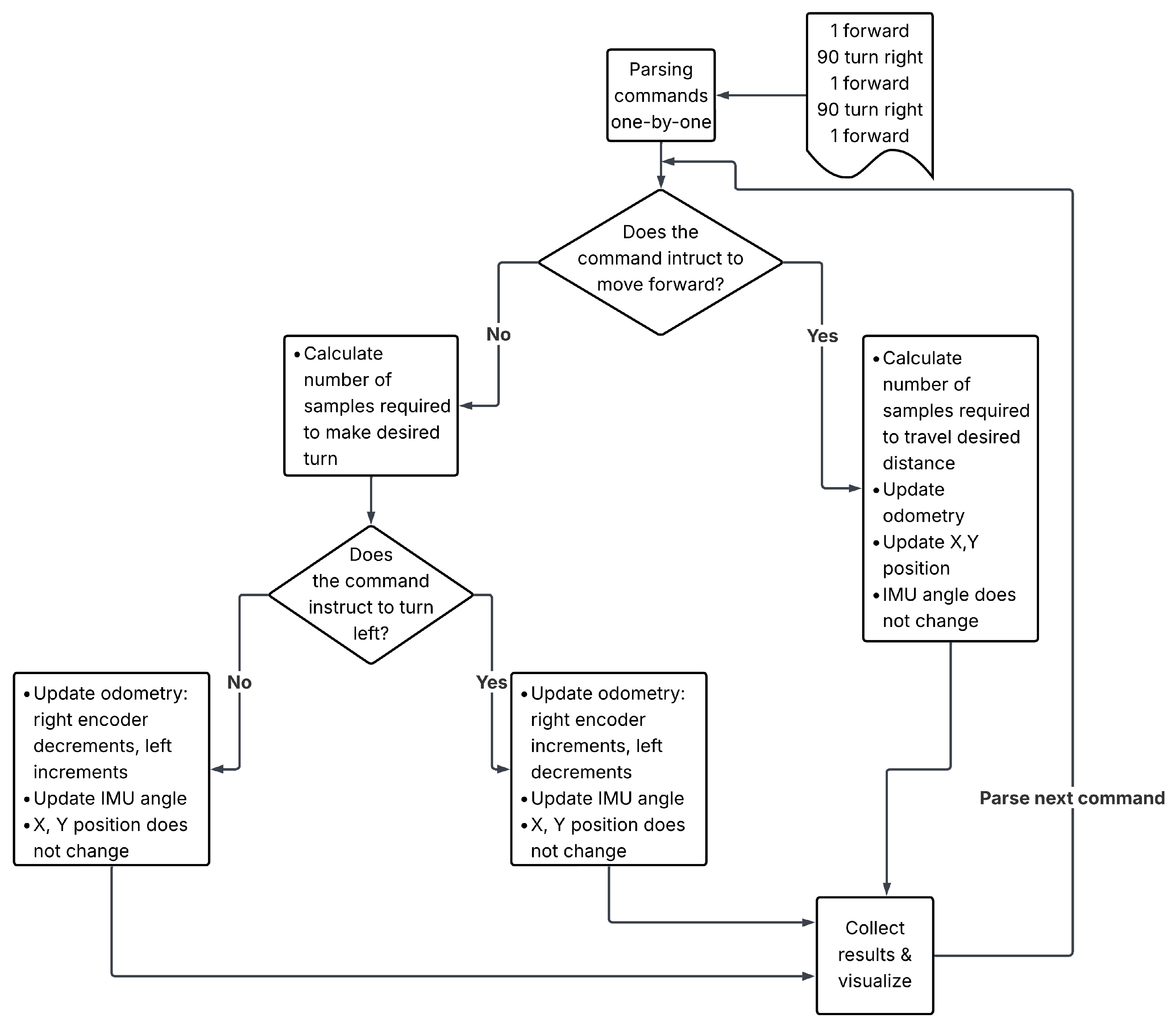
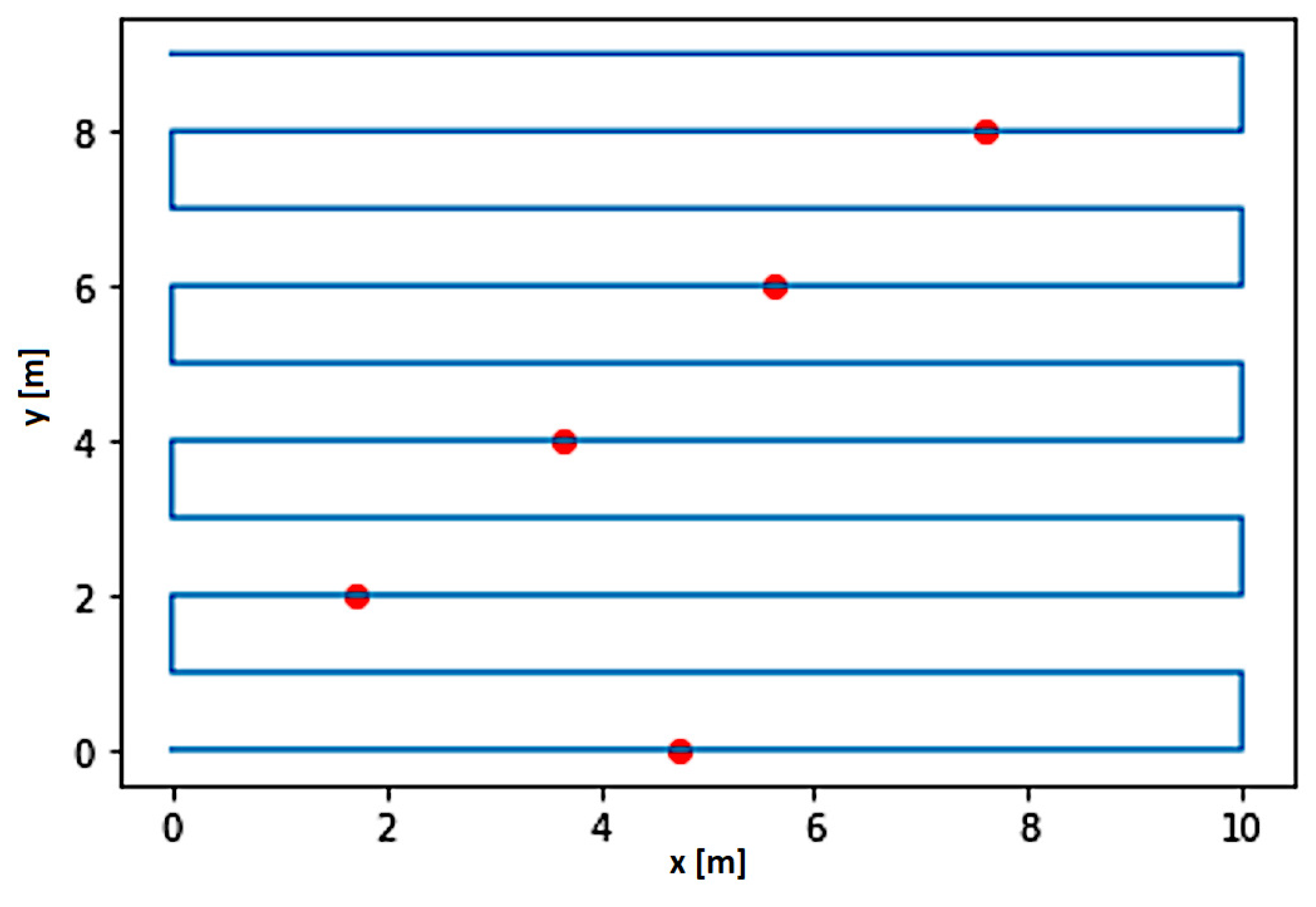
Due to the small amount of data provided from the robot’s test runs and the lack of reference robot routes in these data that would allow for the evaluation of the quality of the proposed algorithm’s operation, a measurement data simulator was developed. The simulator generates synthetic sensor outputs based on a sequence of movement instructions and the characteristics of the robot used in tests. These characteristics include the dimensions of the robot’s wheels, its speed, encoder resolution, and sampling rate. Movement commands include distance, both left and right encoders readings updated incrementally based on distance traveled, and speed and encoders characteristics. Rotation commands include desired angle, and the rotation is simulated by adjusting one encoder upwards and second downwards—left or right—based on desired direction. At the same time, the IMU angle is updated. The X and Y position of the robot stem from simulated odometry and IMU angle. The block diagram is presented in Figure 7. The simulator allows for added slippages as a post-processing step.

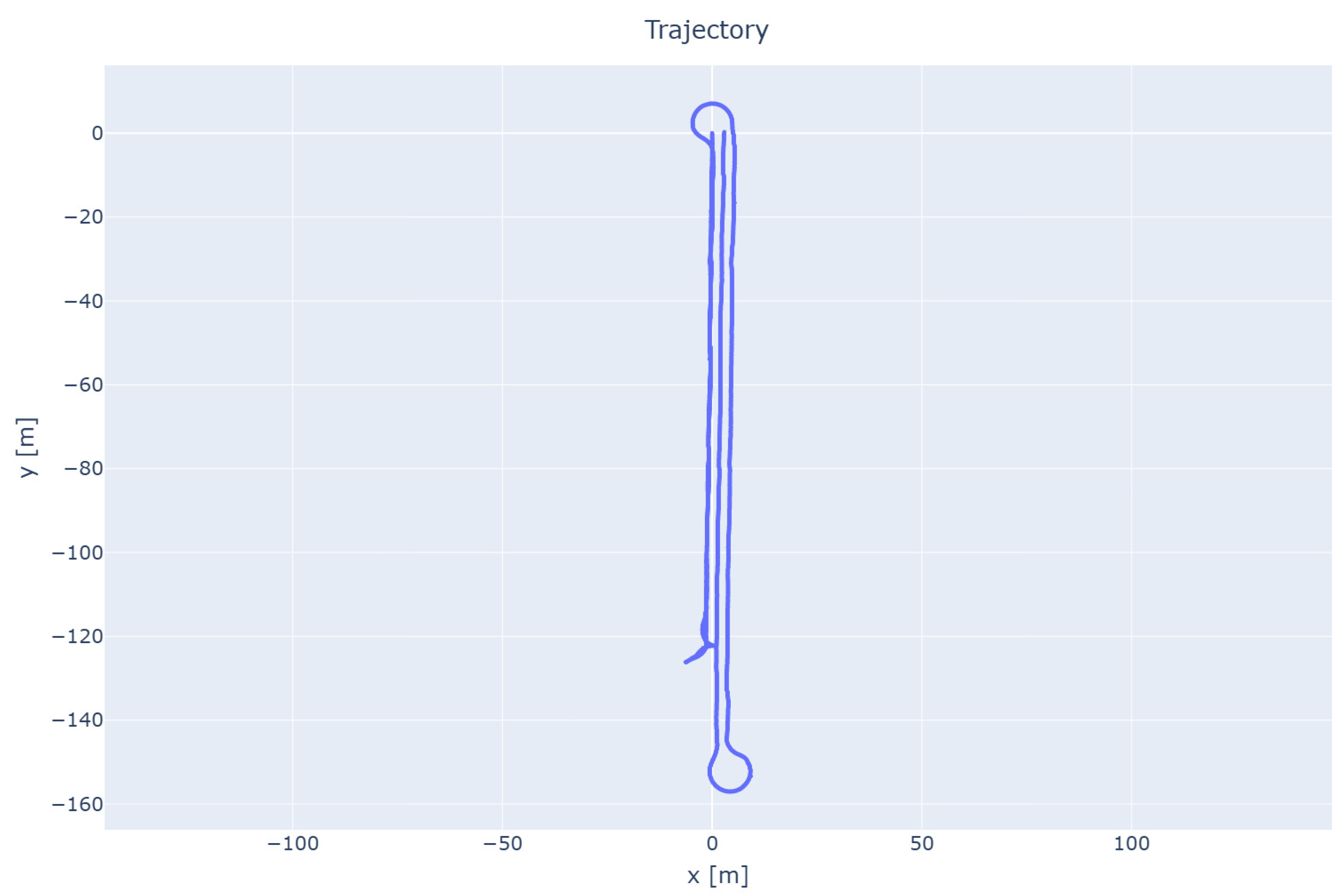
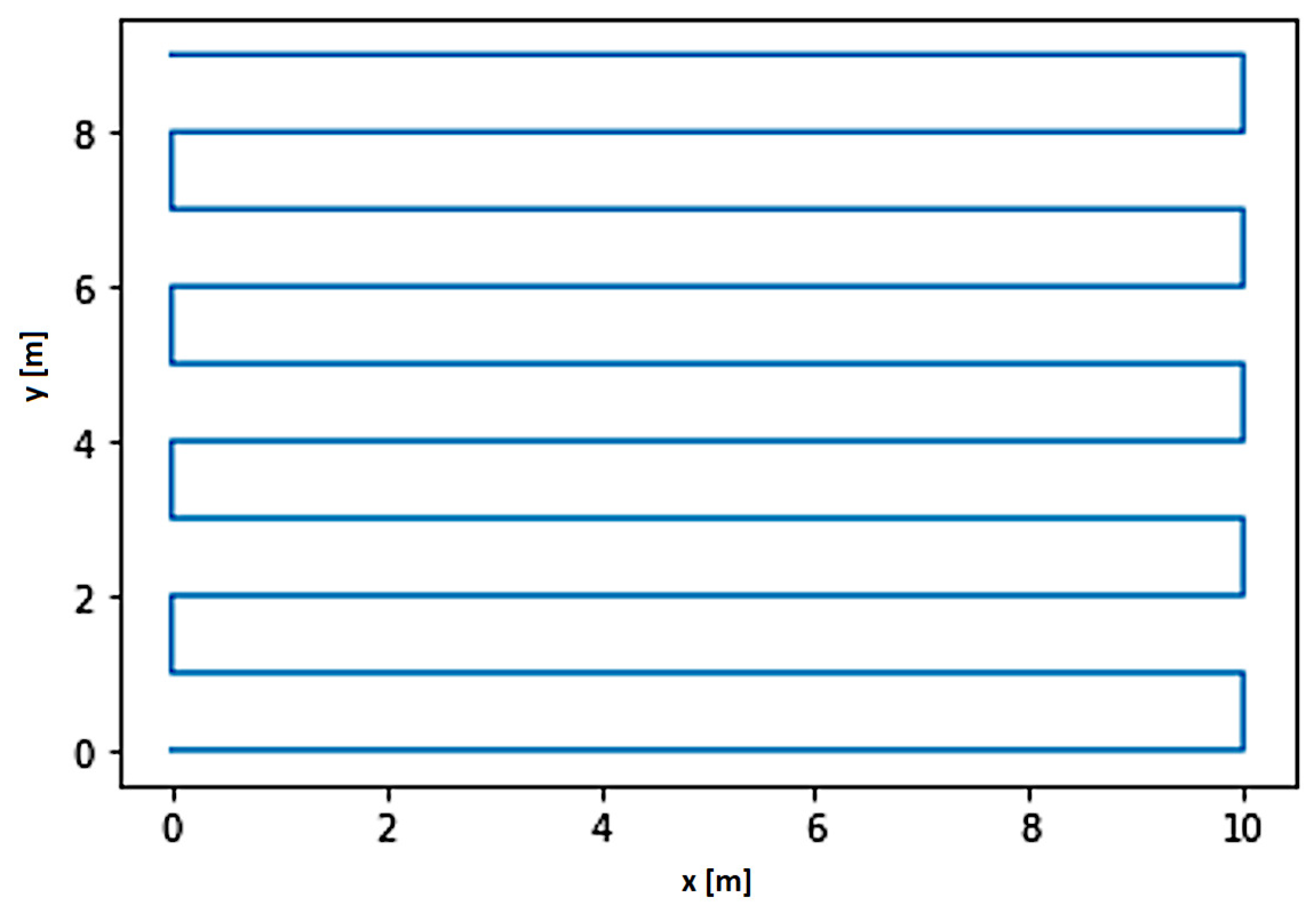
The reference route designated using the simulator is shown in Figure 8.

Slippages were simulated in the simulator, as shown in Figure 9.

The route determined only by formulas that take into account the positions of the encoder (to show that the slippages have been simulated) is shown in Figure 10.

6. Experiments on Rosario Data Set

The first stage of the work focused on understanding the basic problems related to determining the position of objects. For this purpose, several experiments were conducted on publicly available data (Rosario dataset). The conclusions and experience gained allowed us to prepare both a simulation environment and to construct a predictive model for determining the robot’s position based on data from the IMU module, also taking into account possible slippages while driving.

6.1. Gradient Boosting Experiments

For the experiments on the Rosario data, the following set of input independent variables was assumed:

• time stamp,
• latitude in degrees,
• longitude in degrees,
• linear in m/s based on odometry data,
• angular velocity in rad/s based on IMU data,
• linear acceleration in m/s² based on IMU data,
• position on the X-, Y-, and Z-axis based on odometry data,
• orientation in free space in the form of quaternions based on odometry data.

Based on the data from the odometry, dependent variables were prepared for ML models, defining the change in the robot’s position relative to the previous location (length of the displacement vector and angle). The length of the vector was determined as the difference in displacement from the previous location to the current position. The Euclidean distance formula was used to determine the length of the displacement vector:

$$d(A,B)=\sqrt{{(x_B-x_A)}^2+{(y_B-y_A)}^2}$$

(1)

To determine the value of the azimuth angle, the following formulas were used, which allowed for calculating the azimuth of two points (A and B):

$$\begin{array}{c}dx=x_B-x_A\\ dy=y_B-y_A\\ {\displaystyle \phi =\left({\displaystyle arctan\frac{dy}{dx}}\right)·\frac{180}{\pi }}\end{array}$$

(2)

Then, depending on the quadrant of the coordinate system in which the angle is located, one of the following formulas should be used to determine the exact azimuth value:

$$\begin{array}{c}{A}_{AB}={\phi }_I\hfill \\ A_{AB}={180}^{\circ }-{\phi }_{II}\hfill \\ A_{AB}={180}^{\circ }+{\phi }_{III}\hfill \\ A_{AB}={360}^{\circ }-{\phi }_{IV}\hfill \end{array}$$

(3)

The subscript in the angles denotes the quadrant of the coordinate system in which the angle is located. In the above formulas, the orientation of the axes is assumed to be consistent with the geodetic coordinate system (the X-axis is directed vertically upward, and the Y-axis is directed horizontally to the right). Similarly to the vectors and azimuth angles from the odometry data, the displacement length and the azimuth angle between the GPS coordinates were also determined based on the GPS sensor. Unfortunately, due to the previously described problems with determining the correct angles based on odometry data, a temporary solution was used that allowed for full implementation of the research. In the case where the calculated rotation angles had too large discrepancies with the data obtained from the GPS sensor (when the difference was at least 20 degrees), instead of the odometry angles, the GPS angles were determined for the set, which were subjected to distortions, to ensure the independence of the model from the location data. The finally prepared dataset consisted of the following variables:

• timestamp,
• latitude in degrees,
• longitude in degrees,
• linear velocity in m/s based on odometry data,
• angular velocity in rad/s based on IMU data,
• linear acceleration in m/s² based on IMU data,
• position on X-, Y-, Z-axis based on odometry data,
• orientation in free space in quaternions based on odometry data,
• length of displacement vector in XY plane, based on odometry data,
• azimuth angle based on odometry data,
• change of position on X axis, based on odometry data,
• change of position on Y axis, based on odometry data,
• length of displacement vector in XY plane, based on GPS data,
• azimuth angle, based on GPS.

The Gradient Boosting model was chosen to implement the prediction. Two models were used in the research; one predicts the length of the displacement vector and the other the angle of rotation between the historical location and the current position of the robot. The models created in this way were trained on a set of training data, with which models with accuracy were obtained, as presented in

Table 3. Basic statistics describing the regression error on the training and test sets.

Statistic	Training Set	Test Set
Min	0.0074 m	0.0577 m
Max	2.7291 m	4.0601 m
Mean	1.0229 m	2.2941 m
Std	0.7018 m	0.9198 m

. Despite the use of two models, they were evaluated together, as is presented in the table below. To evaluate the models, the predictions they obtained (length of displacement vector and angle of rotation) were converted to subsequent positions of the robot. On the newly determined positions, Euclidean distances were calculated between the robot’s location resulting from GPS data and the positions determined by the predictive models. The calculated locations were determined point by point, so errors in position prediction could accumulate.

In order to better illustrate the improvement in device positioning (based on current odometry and trained models), the next two figures show a comparison of the actual traces (first—Figure 11, and second—Figure 12) and the predictions obtained using Gradient Boosting.

The above figures clearly demonstrate that the use of Gradient Boosting-based prediction significantly improves position prediction compared to odometry-based data alone (Figure 5 and Figure 6).

6.2. Kalman Filter Application

The Kalman filter experiments were conducted on a slightly different set of input data than in the case of Gradient Boosting. The list of variables was as follows:

• time of position recording,
• height relative to the WGS 84 ellipsoid,
• latitude in degrees,
• longitude in degrees,
• position on the X-axis based on odometry measurements,
• position on the Y-axis based on odometry measurements,
• position on the Z-axis based on odometry measurements,
• change in position on the X-axis based on GPS location,
• change in position on the Y-axis based on GPS location,
• shift in the XY plane based on GPS location,
• shift direction based on GPS location,
• change in position on the X-axis based on odometry,
• change in position on the Y-axis based on odometry,
• shift in the XY plane based on odometry,
• shift direction based on odometry.

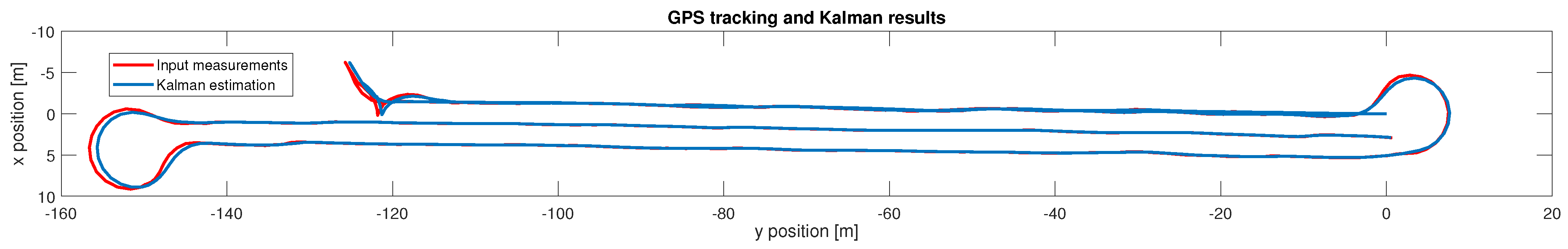
In the experiments, two independent one-dimensional filters were used for each of the X and Y directions separately. Figure 13 shows the actual course of the pass (red) with the Kalman filter response superimposed.

Since the displacement was determined based on two signals ($dx$ and $dy$), it is worth illustrating how the prediction errors of both signals are related independently of each other. The graph below (Figure 14) shows two series for each of these variables: the continuous line (red for $dx$ and blue for $dy$) shows the value of the difference between the change in position based on GPS and the change in position resulting from prediction (these differences can be both positive and negative), while the dashed line (the same colors are maintained) shows the absolute value of these differences.

The purpose of generating this graph was to illustrate whether errors are repeatable (the graph of differences tends to be on only one side of the X axis, below or above) or whether these differences are characterized by frequent sign changes. This is important in the context of a possible accumulation of errors. In the second case (differences often change sign), the cumulative error (difference in position in the longer observation horizon) will be smaller than if the sum of absolute values of differences from each measurement was determined.

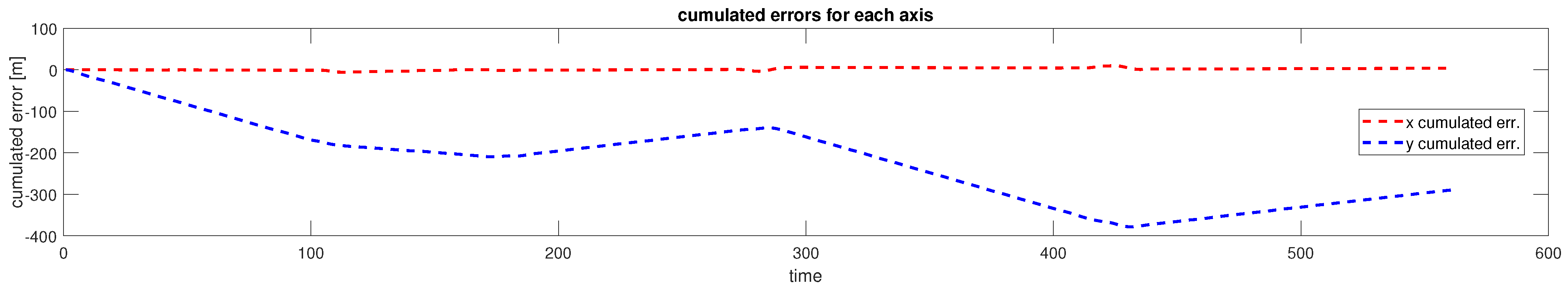
The last graph (Figure 15) shows the comparison of the cumulative position prediction error for each of the variables ($dx$ and $dy$).

However, it should be remembered that this cumulative error should also be related to the nature of the trip. As shown earlier (Figure 11), the first trip was vertical, which caused small changes in the X direction. Hence, the position forecasts had a chance to be more accurate than in the case of the forecasts for the Y direction. This is an important remark because for subsequent trips, their orientation is completely opposite: they generally take place along the X axis.

The preliminary results obtained based on the use of the Kalman filter allow us to assume that this method can be a valuable complement to ML models. In practice, for almost all trips (except the fourth), we observe a tendency to reduce the cumulative error in determining the position relative to the dominant axis. We expect that the use of a mixed model (Kalman filter used for odometry data with a time-corrected position based on GPS) would significantly increase the accuracy of determining the vehicle’s location.

6.3. Deep Learning Approach

The starting point for creating data for deep learning methods was the set defined for the Gradient Boosting method. Before directly creating models, these data were subjected to normalization, as it was expected that this could significantly improve the quality of the obtained results. In the next step, the dataset was divided into a training set (70%), validation set (15%), and test set (15%).

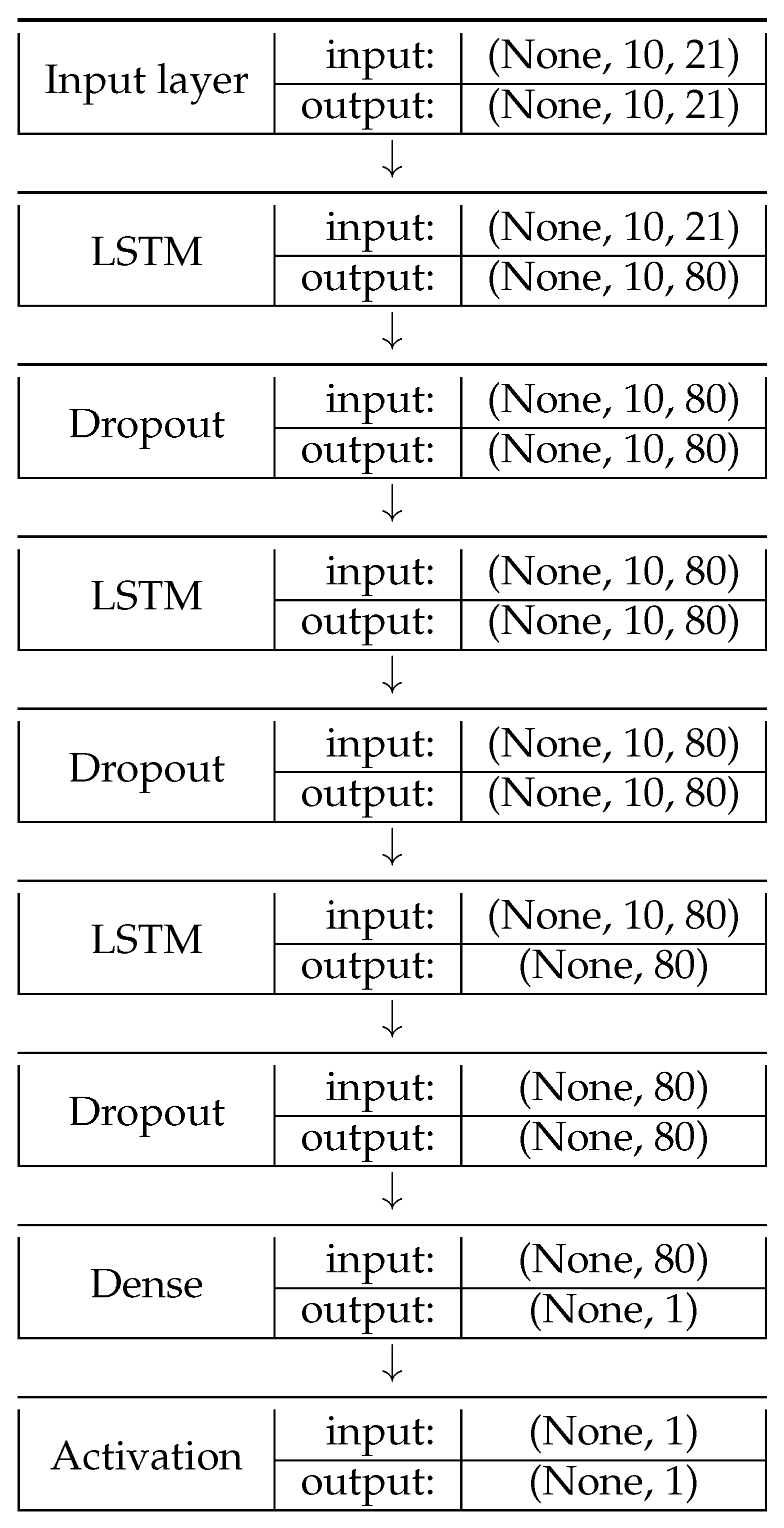
A neural network model prepared on the basis of the Telemanom architecture was used to predict the robot’s routes at this stage. The proposed neural network consists of 3 LSTM (Long Short-Term Memory) layers, 3 dropout layers, and an output layer with one neuron, which allows for the prediction of an expected value. LSTM layers are recurrent layers that use sequential information, which is why they are very good for time-series analyses. Dropout layers allow for the removal of neurons with a given probability, which allows for minimizing the overfitting phenomenon, i.e., excessive matching to the input data. Below (Figure 16) is a diagram of the neural network used to perform route forecasting analyzes.

Initially, one neural network was used to predict the robot’s position, but after conducting the tests (and due to the characteristics of the input data), two neural networks with an identical structure were used, but predicting two different variables: the length of the shift and the angle of rotation.

The deep learning model assumed four variants of position correction based on the GPS signal. This correction was performed every 60, 30, 15 s, or not at all. The results obtained for individual frequencies based on the Rosario set are presented below (

Table 4. Prediction accuracy (error statistics) for position correction every 60 s.

Model	Set	Min [m]	Max [m]	Mean [m]	Std [m]	Variance [m2]
shift prediction	training	0.0035	7.6107	2.5564	1.6572	2.7464
	validation	0.3448	8.1166	2.8856	2.0974	4.3989
	test	1.6974	9.9814	6.1868	2.0326	4.1314
rotation angle prediction	training	0.0016	5.7101	2.3974	1.0948	1.1985
	validation	0.2284	9.7487	2.9950	2.3211	5.3877
	test	1.1061	13.2860	5.3638	3.6709	13.4752
combined models	training	0.0175	7.0544	3.1136	1.7321	3.0001
	validation	0.0695	11.1422	2.775	2.8718	8.2473
	test	0.1693	15.5186	8.3503	3.3219	11.0349

,

Table 5. Prediction accuracy (error statistics) for position correction every 30 s.

Model	Set	Min [m]	Max [m]	Mean [m]	Std [m]	Variance [m2]
shift prediction	training	0.0105	10.6361	4.274	2.7175	7.3847
	validation	1.2245	7.1529	3.6722	1.561	2.4366
	test	1.7229	9.7092	5.6022	1.7251	2.9761
rotation angle prediction	training	0.0014	23.4485	7.9050	5.3895	29.0466
	validation	0.2247	15.3231	3.8786	3.9605	15.6853
	test	1.1578	23.9064	14.847	6.0897	37.085
combined models	training	0.0115	23.4357	8.3242	5.7318	32.8538
	validation	0.0179	14.3587	4.9845	3.2369	10.4773
	test	0.2142	25.0054	15.4801	6.4111	41.1016

,

Table 6. Prediction accuracy (error statistics) for position correction every 15 s.

Model	Set	Min [m]	Max [m]	Mean [m]	Std [m]	Variance [m2]
shift prediction	training	0.0105	7.8896	2.7234	1.8481	3.4153
	validation	0.6755	5.9189	2.8521	1.1914	1.4194
	test	1.6229	5.3765	3.1913	0.8747	0.7650
rotation angle prediction	training	0.0015	29.2632	10.0861	6.7744	45.8919
	validation	0.2284	21.7601	11.8091	7.3604	54.1752
	test	1.1036	22.0759	10.175	7.381	54.4799
combined models	training	0.0168	30.5053	10.6629	7.266	52.7952
	validation	0.1651	21.9581	11.87	7.4058	54.8463
	test	0.0407	22.2574	10.3826	7.3307	53.7387

and

Table 7. Prediction accuracy (error statistics) without any correction.

Model	Set	Min [m]	Max [m]	Mean [m]	Std [m]	Variance [m2]
shift prediction	training	0.0022	6.3867	2.2806	1.4253	2.0315
	validation	0.3080	8.6515	3.9437	2.8128	7.9121
	test	0.4223	6.7295	2.2725	1.1842	1.402
rotation angle prediction	training	0.0032	8.9287	3.9507	2.1348	4.5575
	validation	0.2219	7.6648	2.8990	1.4940	2.2320
	test	0.3452	6.6037	2.4043	1.8275	3.3399
combined models	training	0.0051	9.4925	4.5171	2.4439	5.9727
	validation	0.0238	8.6200	4.5962	2.3534	5.5383
	test	0.0858	8.0750	2.8266	2.7217	7.4075

).

The rows describing the models predicting the displacement length and rotation angle refer to individual models, while the last rows of the table define the total evaluation of the models. In order to enable the evaluation of the models, the predictions obtained by them (displacement vector length and rotation angle) were iteratively recalculated to subsequent robot positions. Based on subsequent robot positions, Euclidean distances were determined between the expected data and the positions determined using the neural network model. Positions were recalculated iteratively, so prediction errors may accumulate.

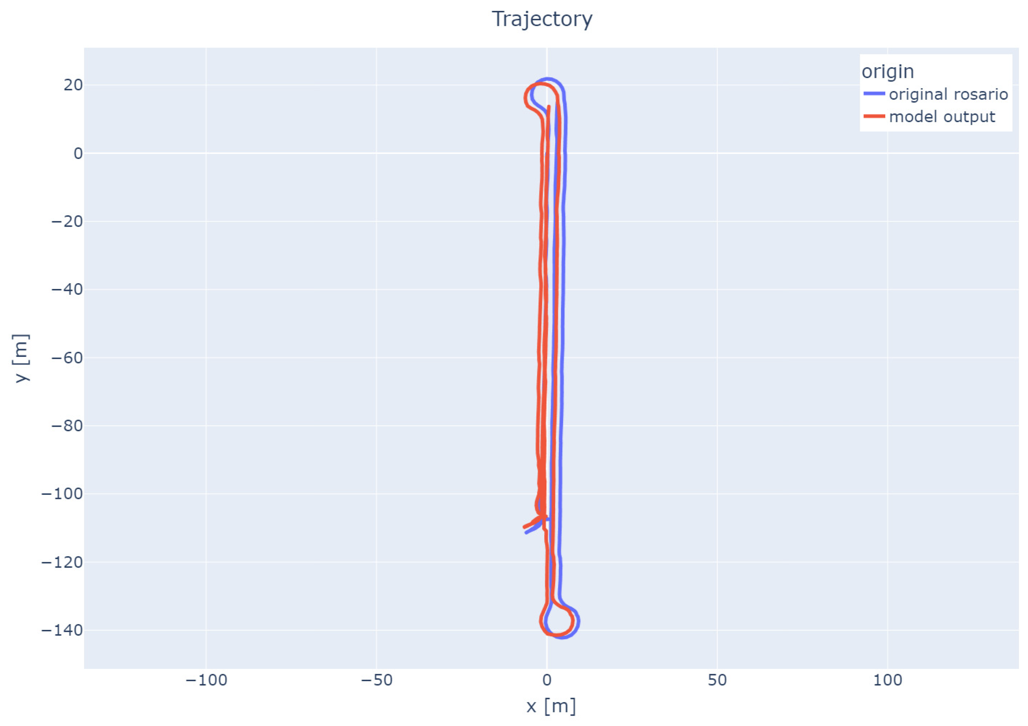
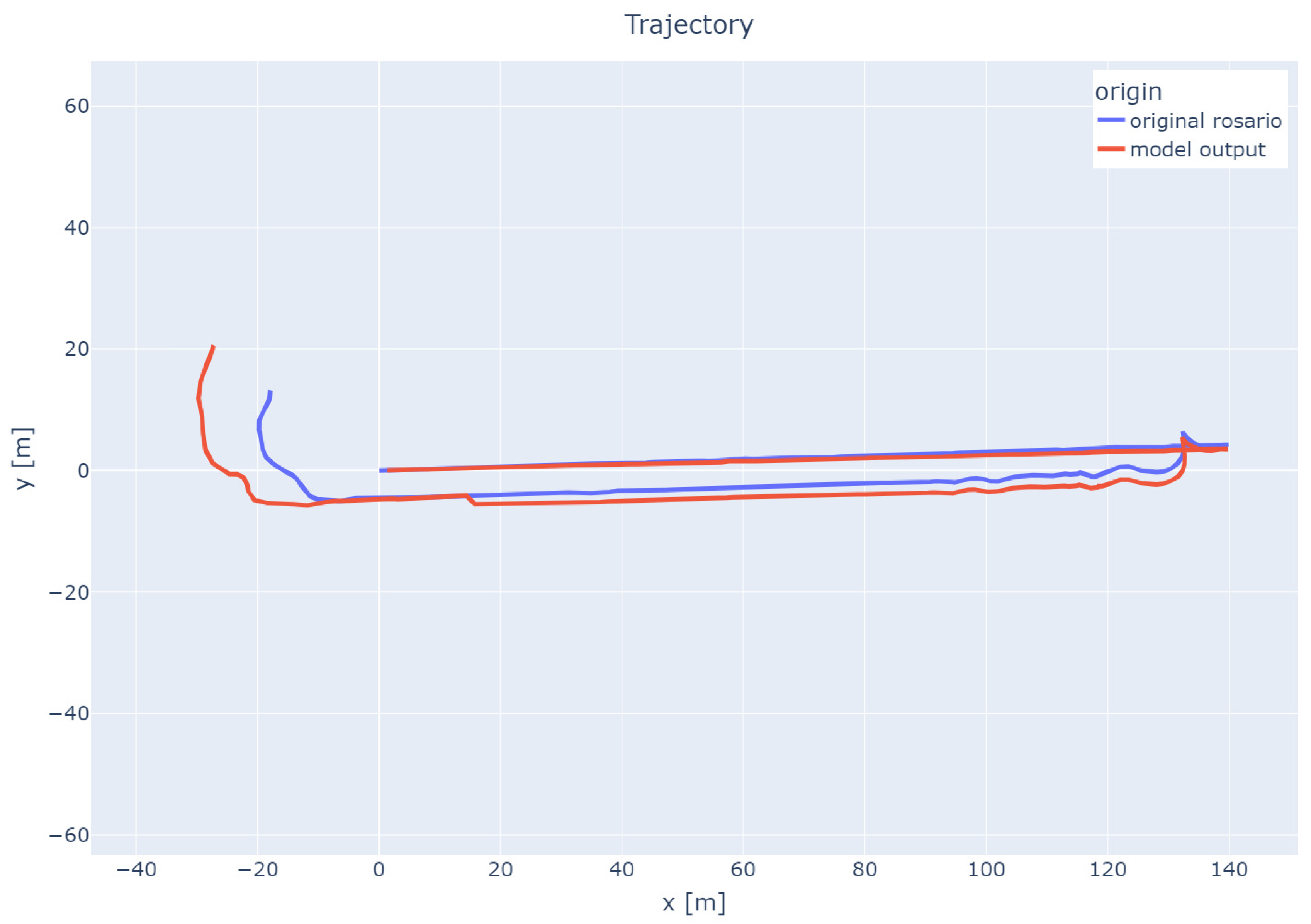
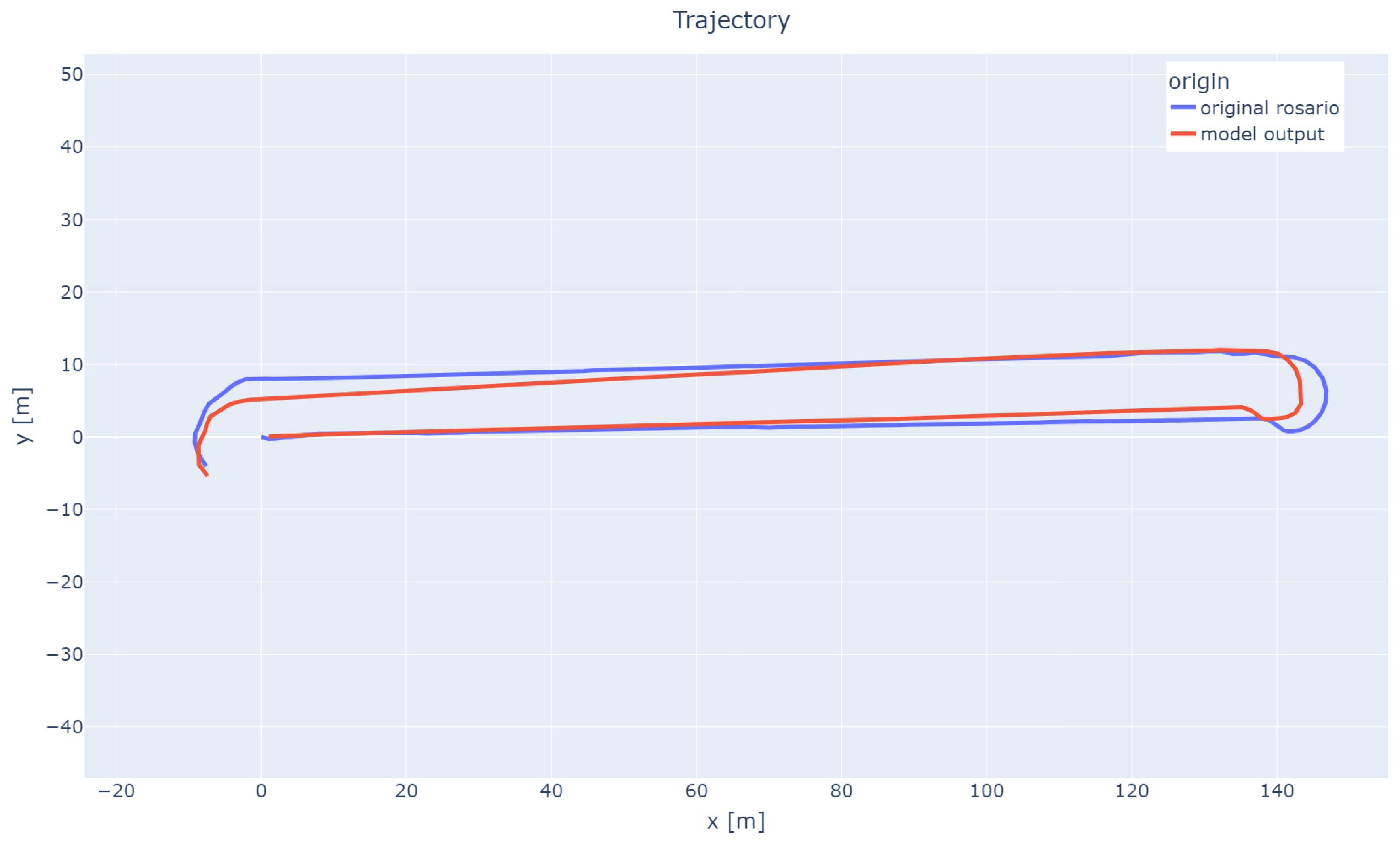
Based on the prepared neural network models, predictions of the robot’s travel routes were made on the basis of odometry data and data from IMU sensors. The following Figure 17, Figure 18 and Figure 19 show the selected predicted travel routes (without an additional navigation signal in the input data) together with the actual route determined based on GPS data. The route determined based on GPS data is marked in blue, while the predicted travel route is marked in red.

7. Experiments on Domain Data Sets

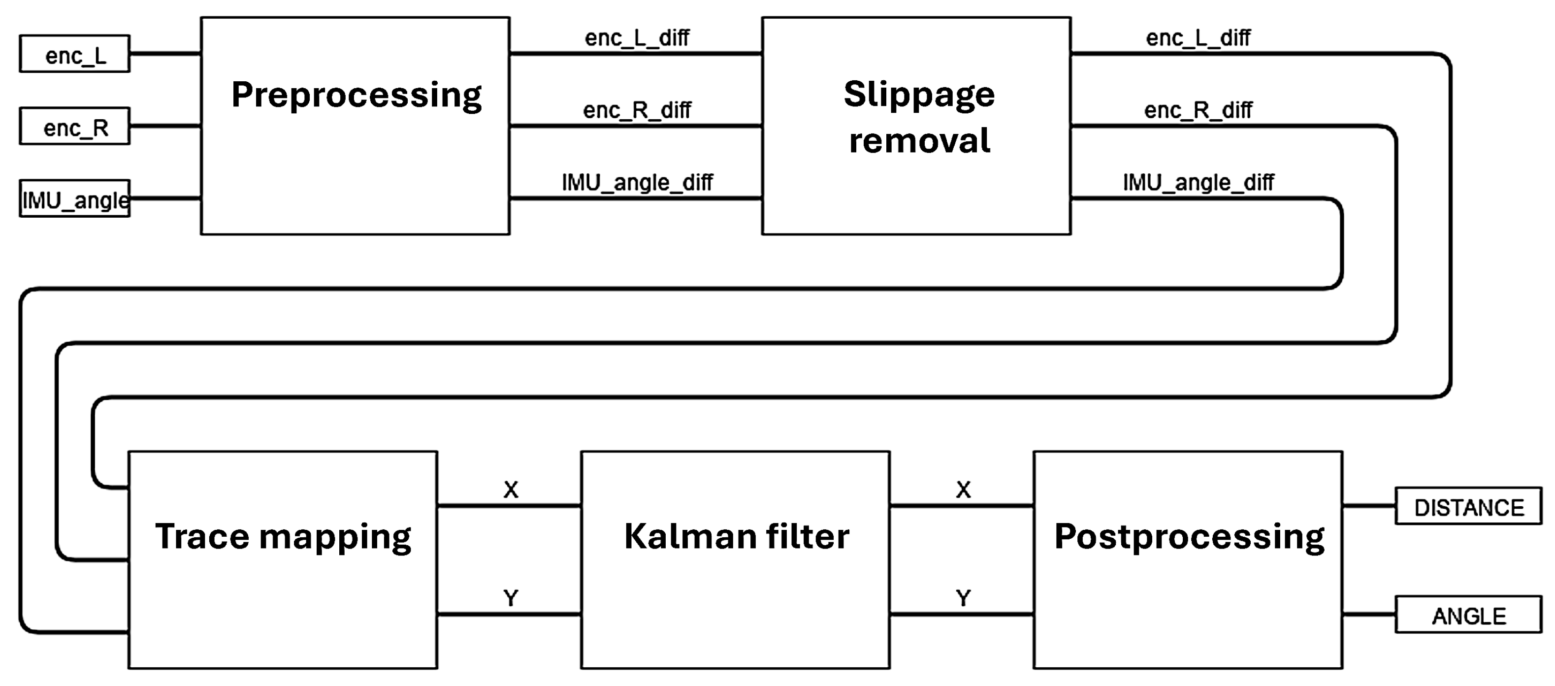
Ultimately, a robot positioning algorithm was created based on odometry data and IMU sensor data using the classical method, that is, using formulas defining robot displacements based on data from these sensors. Additionally, in addition to determining the robot position based on appropriate calculations, the algorithm was enriched with a module to preprocess measurement signal data to protect the solution against unusual situations and a module to remove slippages. The algorithm also uses a Kalman filter, which allows for estimating the robot position based on data that may be burdened with error. The algorithm scheme is shown in Figure 20.

The algorithm works in a follow-up manner, i.e., it receives signals from sensors in successive moments and returns information on the output about how much and in what direction the robot has moved since the last measurement. The algorithm consists of the following stages:

• preprocessing;
• slip removal;
• position determination.

The data pre-processing stage begins with the selection of the signals provided, which are used in the algorithm. Then, from the odometry signals, values are determined as to how much the position of individual encoders has changed since the last sample, and from the IMU sensor signal, the change in the robot’s position angle on the ship’s side is determined. These signals are then validated to detect unusual situations, such as excessive changes in IMU or encoder measurements, which may indicate robot problems.

The next stage is the wheel slip removal algorithm. Wheel slip is a situation in which slippage occurs between the wheel and the ground—the wheel rotates, but the robot does not move. The encoder of such a wheel indicates that the wheel has moved a certain distance when in fact the wheel has not moved or has moved a smaller distance. Slippage-related errors accumulate and have a significant impact on the route determined based on the encoder readings. This is a known problem for determining the position using odometry. It is therefore important to detect the moments in which slippage occurred and to correct the encoder readings. In the proposed slip removal module, it was possible to correlate the information from the change in the encoder position with the information about the change in the robot’s position angle in the time sample. Based on the change in the encoder position, it is possible to calculate the angle by which the robot has rotated. By comparing the calculated angle with the change in the robot’s position angle read from the IMU sensor, it is possible to detect a situation when the encoder readings are distorted. In such a situation, slippage has occurred and the difference in the encoder positions is corrected.

The last stage is to determine the robot’s position based on the encoders and IMU sensor readings. To determine the position, calculations are performed on the basis of the following formulas:

$$\begin{array}{ccc}\hfill \Delta x& =& \Delta scos\left(\theta +{\displaystyle \frac{\Delta \theta }{2}}\right)\hfill \\ \hfill \Delta y& =& \Delta ssin\left(\theta +{\displaystyle \frac{\Delta \theta }{2}}\right)\hfill \\ \hfill \Delta \theta & =& {\displaystyle \frac{\Delta s_R-\Delta s_L}{2L}}\hfill \\ \hfill \Delta s& =& {\displaystyle \frac{\Delta s_R+\Delta s_L}{2}}\hfill \\ \hfill X_t=f(x,y,\theta ,\Delta s_R,\Delta s_L)& =& \left[\begin{array}{c}x\\ y\\ \theta \end{array}\right]+\left[\begin{array}{c}{\displaystyle \frac{{\displaystyle \Delta s_R+\Delta s_L}}{2}}cos\left(\theta +{\displaystyle \frac{\Delta \theta }{2}}\right)\\ {\displaystyle \frac{{\displaystyle \Delta s_R+\Delta s_L}}{2}}sin\left(\theta +{\displaystyle \frac{\Delta \theta }{2}}\right)\\ {\displaystyle \frac{{\displaystyle \Delta s_R-\Delta s_L}}{2L}}\end{array}\right]\hfill \end{array}$$

(4)

where:

• $\Delta x$—change in robot position in X-axis;
• $\Delta y$—change in robot position in Y-axis;
• $\Delta s_R$—distance covered by the right wheel of the robot;
• $\Delta s_L$—distance covered by the left wheel of the robot;
• $\Delta s$—approximate distance covered by the robot;
• $\Delta \theta$—change in robot position angle;
• $2L$—distance between robot wheels.

In these formulas, the change in the angle of position of the robot $\Delta \theta$ is calculated on the basis of the distance covered by the wheels over a time interval. In the event of slippage, the distances covered by the wheels will be distorted, which will also distort the change in angle. Instead of determining $\Delta \theta$ based on the distance covered by the wheels, it was decided to determine $\Delta \theta$ based on the IMU sensor readings. In the event of slippage, the robot’s movement angle will be maintained, and only the distance will be distorted, which is acceptable in the case of small distances covered by the robot between successive samples. This is particularly important when the robot turns. This is an additional safeguard in the event that the slippage detection module does not detect slippage.

Figure 8, Figure 9 and Figure 10 provided information on how the course was generated, slippages were introduced, and how the run was reproduced without taking slippages into account. Based on the correction developed in the model, it was possible to significantly improve the reproduction of the slippage run, as shown in Figure 21.

Since the simulator, in addition to the simulated signals, the actual route that the simulated robot has ridden also returns, and it is possible to check how much the designated route deviates from the actual route of the robot.

Table 8. Comparison of the route determined by the algorithm with the reference route.

	X Axis [m]	Y Axis [m]
Minimal difference	0.00000	0.00000
Maximal difference	0.00556	0.00560
Average difference	0.00276	0.00000

shows the minimum, maximum, and average differences in the X and Y axes between the actual route and the route designated by the algorithm.

8. Conclusions

In this work, we presented an approach to improving the positioning accuracy of autonomous ship hull-cleaning robots operating in underwater environments. By combining classical kinematic models with modern sensor data processing techniques, we have demonstrated the potential to mitigate the cumulative errors inherent to odometry-based positioning, particularly those caused by wheel slippage.

Our experimental evaluations on the Rosario dataset and in simulation environments have shown that the Gradient Boosting models can correct the displacement and heading errors that arise from pure odometry estimates. Compared to the uncorrected odometry trajectory, both the Gradient Boosting and deep learning approaches yielded improved alignment with the GPS reference route. The deep learning model, using sequential LSTM layers, showed promising results in forecasting both displacement vectors and rotation angles over varying GPS-based correction intervals. Although prediction errors accumulate over time, the ability to periodically correct the trajectory with GPS data resulted in an overall reduction of the accumulated error. Our experiments also highlighted the importance of periodic position corrections, with different correction frequencies revealing trade-offs between computational complexity and positioning accuracy.

We also presented a slip detection and correction module that improved the robot’s ability to maintain accurate positioning despite wheel slippage. The final positioning algorithm, which incorporated preprocessing, slip removal, and sensor fusion, achieved high accuracy with minimal deviations from the reference trajectories in both simulated and real-world tests.

Future work will focus on further validation in real-world maritime environments and the exploration of additional sensor modalities to enhance positioning accuracy and reliability.