
Retinal Vessel Segmentation Using Math-Inspired Metaheuristic Algorithms


Abstract
1. Introduction
- The math-inspired metaheuristic algorithms of CSA, TSA, AOA, GNDO, GOBC-PA, and SCA are implemented for clustering and retinal vessel segmentation.
- The statistical analyses indicate that the considered math-inspired algorithms are able to produce effective results despite their simple algorithmic structures.
2. Materials and Methods
2.1. Circle Search Algorithm
| Randomly create an initial population by, |
| Determine the parameter |
| Cycle = 1 |
| WHILE |
| Calculate the values of the variables , and |
| Calculate the value of |
| Update by using, |
| If Updated solutions are out of the boundaries |
| Set the solutions equal to the boundaries |
| Calculate the fitness value of |
| End |
| Evaluate with the current best solution |
| Update and |
| Cycle = Cycle + 1 |
| END |
2.2. Tangent Search Algorithm
| Randomly create uniformly distributed initial population, |
| Cycle = 1 |
| WHILE |
| Apply Switch procedure for each according to Pswitch |
| If : Intensification phase |
| Produce a random local walk by, |
| Exchange some variables of the obtained solution with the related variables of the |
| current optimal solution by to produce new possible solutions |
| Check the boundaries of the recently produced solutions |
| Repair the overflowed solutions |
| Else : Exploration phase |
| Apply to each variable with a probability equal to 1/D |
| in order to expand the research capacity |
| End |
| Apply Escape Local Minima procedure according a given probability value called Pesc |
| If : Escape local minima phase |
| Randomly select one of the current solutions and apply selection procedures of |
| End |
| Replace with a randomly selected solution having lower fitness value |
| Cycle = Cycle + 1 |
| END |
2.3. Arithmetic Optimization Algorithm
| Randomly create an initial population consisting of positions of the solutions, |
| Cycle = 1 |
| WHILE |
| Calculate the fitness value of each solution in the population |
| Determine the best solution so far |
| Update the Math Optimizer Accelerated (MOA) value |
| Update Math Optimizer probability (MOP) value |
| For |
| For |
| Produce a random values between [0, 1] for the conditions of r1, r2 and r3 |
| If : Exploration phase |
| If |
| Apply Division math operator (D “”) and update the position of |
| solution i |
| Else |
| Apply Multiplication math operator (M “”) and update the position of |
| solution i |
| End if |
| Else |
| If : Exploitation phase |
| Apply Substraction math operator (S “”) and update the position of |
| solution i |
| Else |
| Apply Addition math operator (A “”) and update the position of |
| solution i |
| End if |
| End if |
| End |
| End |
| Cycle = Cycle + 1 |
| END |
2.4. Generalized Normal Distribution Optimization Algorithm
| Randomly create an initial population by, and |
| Calculate the fitness value of each solution and determine the best solution as |
| Cycle = 1 |
| WHILE |
| For |
| Produce a random number () in the interval of [0, 1] |
| If : Local exploitation strategy |
| Select the current optimal solution and calculate the mean position M |
| Compute the generalized mean position , generalized standard variances |
| and penalty factor |
| Apply the local exploitation strategy to calculate and |
| Else: Global exploration strategy |
| Apply the global exploration strategy |
| End if |
| End for |
| Cycle = Cycle + 1 |
| END |
2.5. Global Optimization Method Based on Clustering and Parabolic Approximation
| Randomly create an initial population |
| Set the number of cluster size as and maximum epoch size as |
| Calculate the fitness value produced by the objective function |
| For |
| Determine the cluster centers |
| Determine the membership matrix of via clustering |
| Sort the cluster centers with ascending order in accordance with the fitness values |
| Select the first ceil cluster centers as () |
| For |
| Determine the H set which represent the members of taken from depending |
| on |
| If |
| Determine the parabola coefficient matrix () |
| Find the coefficients of approximated parabola () |
| End if |
| End for |
| For |
| Determine the vertex of parabola |
| If , the parabola can be assumed as concave and keep |
| Else if , the parabola can be assumed as convex, and if is better |
| than then replace with |
| Else if is not a number or infinite then keep |
| End if |
| End for |
| Randomly create a new population around the |
| Randomly create new population around the current best two solutions |
| Randomly create a new population |
| Determine as |
| Calculate the fitness value of the objective function by using the new population |
| Determine as the best solution of |
| If , can be defined as the global minimum |
| End if |
| End for |
2.6. Sine Cosine Algorithm
| Randomly create an initial population consisting a set of search agents, |
| Cycle = 1 |
| WHILE |
| Calculate the fitness value of each search agent in the population |
| Determine the best search agent so far and store it in a variable as destination agent |
| Update the random parameters and |
| Update the position of each search agent in the current population |
| Store the current destination point as the best search agent obtained so far |
| Cycle = Cycle + 1 |
| END |
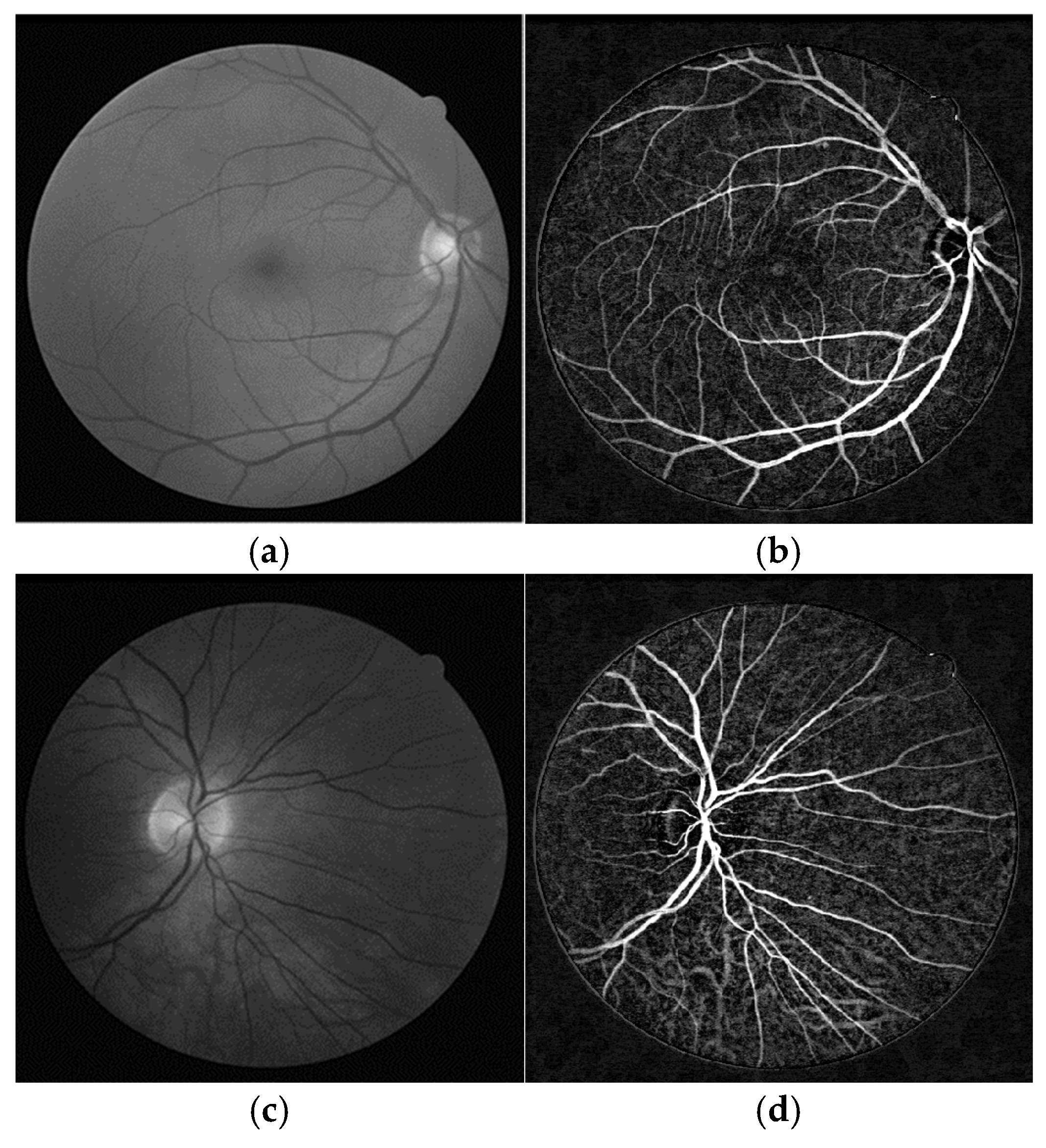
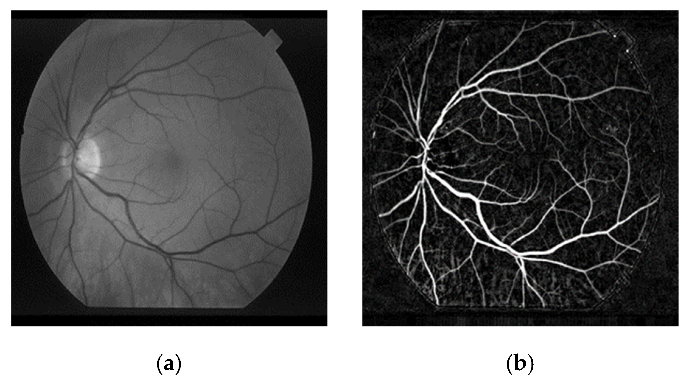
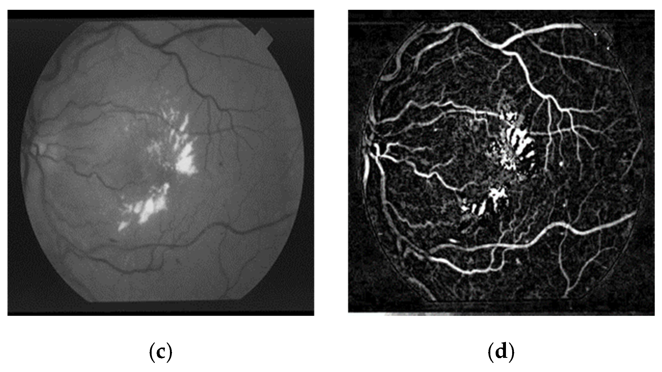
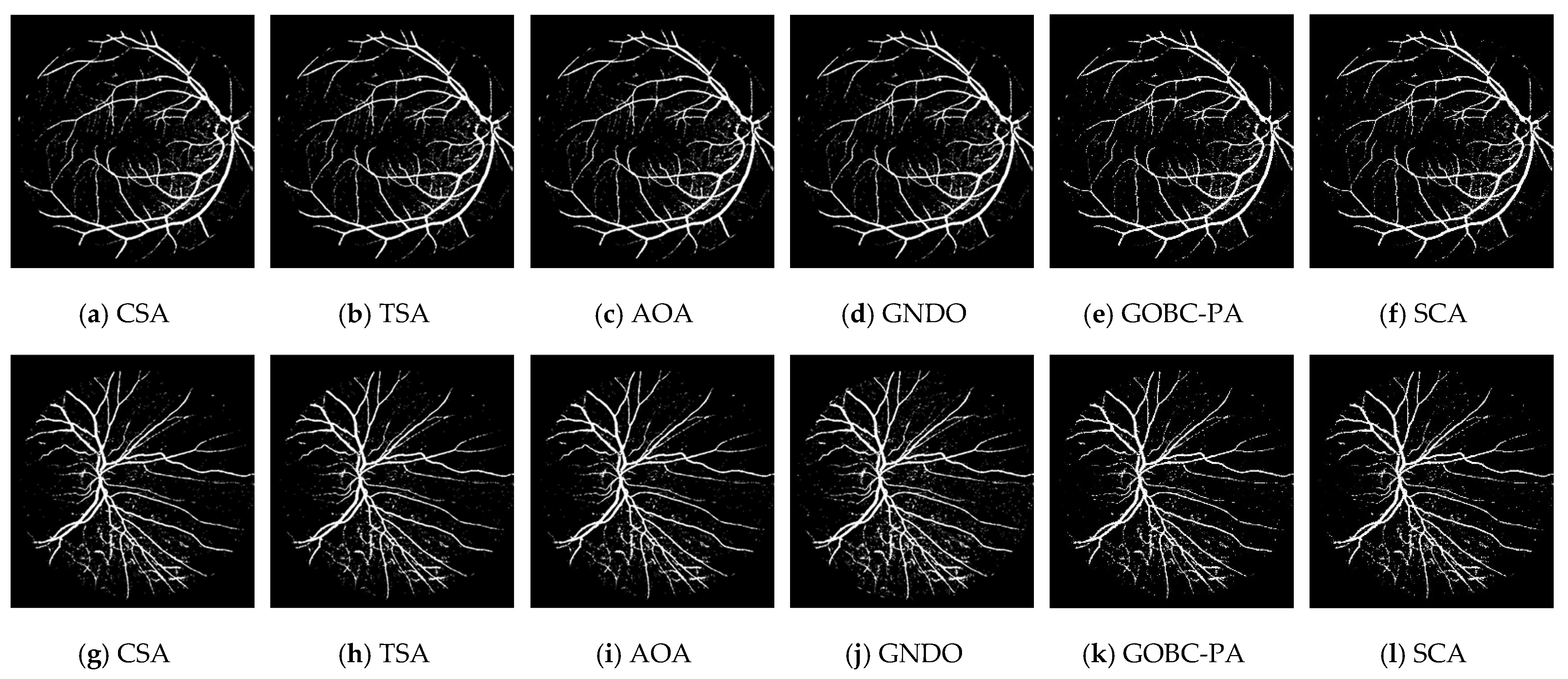
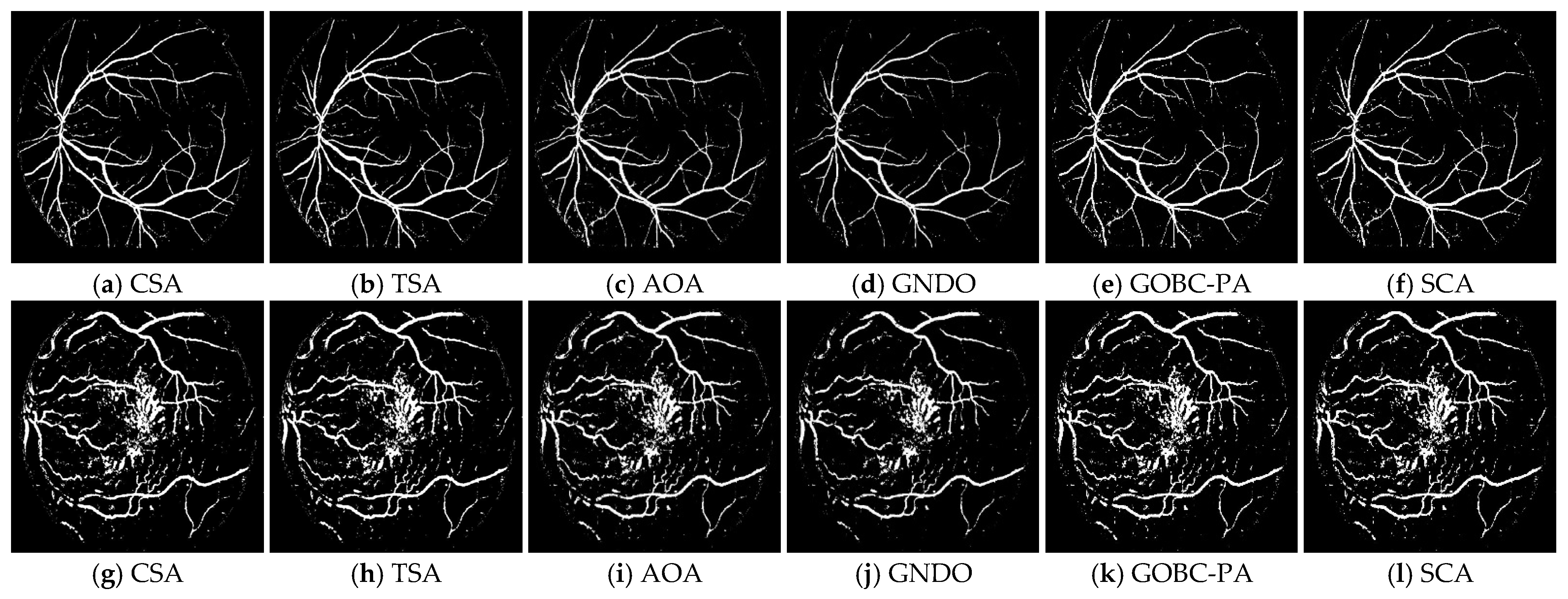
3. Results
3.1. Segmentation Performance
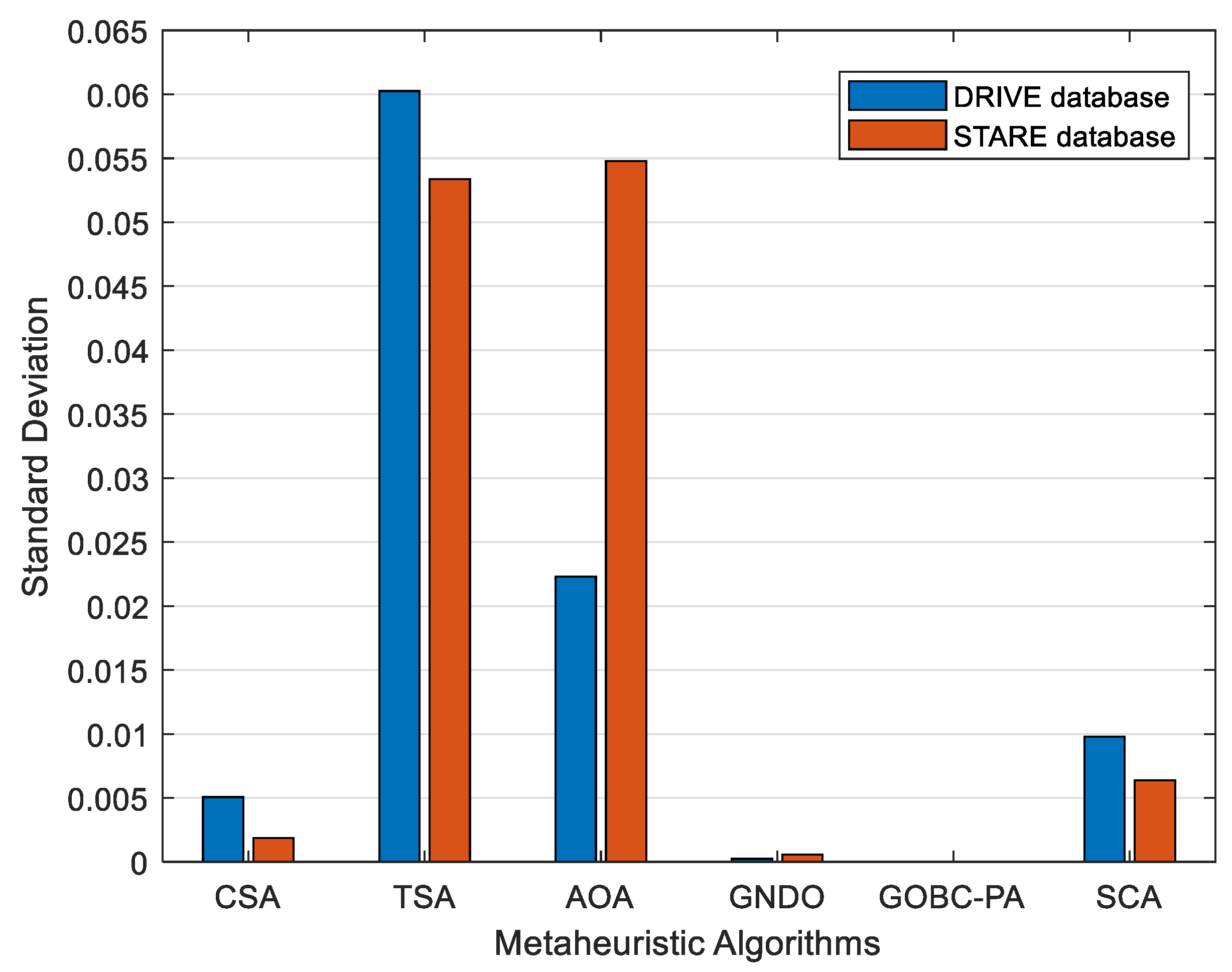
3.2. Statistical Analysis
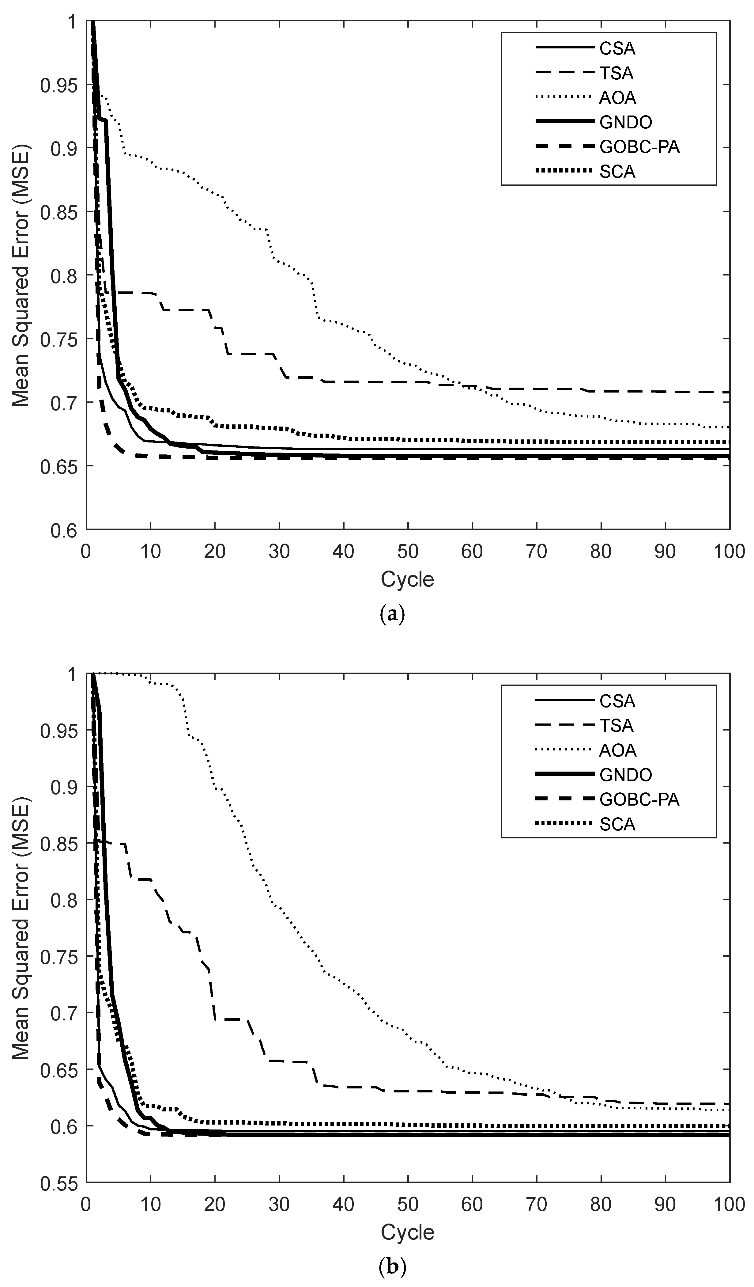
3.3. Convergence Analysis
4. Discussion
Author Contributions
Funding
Informed Consent Statement
Data Availability Statement
Conflicts of Interest
References
- Mirjalili, S. SCA: A sine cosine algorithm for solving optimization problems. Knowl.-Based Syst. 2016, 96, 120–133. [Google Scholar] [CrossRef]
- Layeb, A. Tangent search algorithm for solving optimization problems. Neural Comput. Appl. 2022, 34, 8853–8884. [Google Scholar] [CrossRef]
- Qais, M.H.; Hasanien, H.M.; Turky, R.A.; Alghuwainem, S.; Tostado-Véliz, M.; Jurado, F. Circle search algorithm: A geometry-based metaheuristic optimization algorithm. Mathematics 2022, 10, 1626. [Google Scholar] [CrossRef]
- Abualigah, L.; Diabat, A.; Mirjalili, S.; Abd Elaziz, M.; Gandomi, A.H. The arithmetic optimization algorithm. Comput. Methods Appl. Mech. Eng. 2021, 376, 113609. [Google Scholar] [CrossRef]
- Zhang, Y.; Jin, Z.; Mirjalili, S. Generalized normal distribution optimization and its applications in parameter extraction of photovoltaic models. Energy Convers. Manag. 2020, 224, 113301. [Google Scholar] [CrossRef]
- Pence, I.; Cesmeli, M.S.; Senel, F.A.; Cetisli, B. A new unconstrained global optimization method based on clustering and parabolic approximation. Expert Syst. Appl. 2016, 55, 493–507. [Google Scholar] [CrossRef]
- Gonidakis, D.; Vlachos, A. A new sine cosine algorithm for economic and emission dispatch problems with price penalty factors. J. Inf. Optim. Sci. 2019, 40, 679–697. [Google Scholar] [CrossRef]
- Abdelsalam, A.A. Optimal distributed energy resources allocation for enriching reliability and economic benefits using sine–cosine algorithm. Technol. Econ. Smart Grids Sustain. Energy 2020, 5, 8. [Google Scholar] [CrossRef]
- Babaei, F.; Safari, A. SCA based fractional-order PID controller considering delayed EV aggregators. J. Oper. Autom. Power Eng. 2020, 8, 75–85. [Google Scholar] [CrossRef]
- Mishra, S.; Gupta, S.; Yadav, A. Design and application of controller based on sine–cosine algorithm for load frequency control of power system. In Intelligent Systems Design and Applications; Springer: Cham, Switzerland, 2020; pp. 301–311. [Google Scholar] [CrossRef]
- Algabalawy, M.A.; Abdelaziz, A.Y.; Mekhamer, S.F.; Aleem, S.H.A. Considerations on optimal design of hybrid power generation systems using whale and sine cosine optimization algorithms. J. Electr. Syst. Inf. Technol. 2018, 5, 312–325. [Google Scholar] [CrossRef]
- Bhadoria, A.; Marwaha, S.; Kamboj, V.K. An optimum forceful generation scheduling and unit commitment of thermal power system using sine cosine algorithm. Neural Comput. Appl. 2019, 32, 2785–2814. [Google Scholar] [CrossRef]
- Mirjalili, S.M.; Mirjalili, S.Z.; Saremi, S.; Mirjalili, S. Sine Cosine Algorithm: Theory, Literature Review, and Application in Designing Bend Photonic Crystal Waveguides. In Nature-Inspired Optimizers; Springer: Cham, Switzerland, 2020; pp. 201–217. [Google Scholar]
- Das, S.; Bhattacharya, A.; Chakraborty, A.K. Solution of short-term hydrothermal scheduling using sine cosine algorithm. Soft Comput. 2018, 22, 6409–6427. [Google Scholar] [CrossRef]
- Bhookya, J.; Jatoth, R.K. Optimal FOPID/PID controller parameters tuning for the AVR system based on sine-cosine-algorithm. Evol. Intell. 2019, 12, 725–733. [Google Scholar] [CrossRef]
- Hekimoğlu, B. Sine–cosine algorithm-based optimization for automatic voltage regulator system. Trans. Inst. Meas. Control 2019, 41, 1761–1771. [Google Scholar] [CrossRef]
- Gorripotu, T.S.; Ramana, P.; Sahu, R.K.; Panda, S. Sine cosine optimization based proportional derivative-proportional integral derivative controller for frequency control of hybrid power system. In Computational Intelligence in Data Mining; Springer: Singapore, 2020; pp. 789–797. [Google Scholar] [CrossRef]
- Belazzoug, M.; Touahria, M.; Nouioua, F.; Brahimi, M. An improved sine cosine algorithm to select features for text categorization. J. King Saud Univ. Comput. Inf. Sci. 2020, 32, 454–464. [Google Scholar] [CrossRef]
- Kaur, G.; Dhillon, J.S. Economic power generation scheduling exploiting hill-climbed sine–cosine algorithm. Appl. Soft Comput. 2021, 111, 107690. [Google Scholar] [CrossRef]
- Fan, F.; Chu, S.C.; Pan, J.S.; Yang, Q.; Zhao, H. Parallel sine cosine algorithm for the dynamic deployment in wireless sensor networks. J. Internet Technol. 2021, 22, 499–512. [Google Scholar] [CrossRef]
- Mookiah, S.; Parasuraman, K.; Chandar, S.K. Color image segmentation based on improved sine cosine optimization algorithm. Soft Comput. 2022, 26, 13193–13203. [Google Scholar] [CrossRef]
- Karmouni, H.; Chouiekh, M.; Motahhir, S.; Qjidaa, H.; Jamil, M.O.; Sayyouri, M. Optimization and implementation of a photovoltaic pumping system using the sine–cosine algorithm. Eng. Appl. Artif. Intell. 2022, 114, 105104. [Google Scholar] [CrossRef]
- Jafari, M.; Chaleshtari, M.H.B.; Khoramishad, H.; Altenbach, H. Minimization of thermal stress in perforated composite plate using metaheuristic algorithms WOA, SCA and GA. Compos. Struct. 2023, 304, 116403. [Google Scholar] [CrossRef]
- Chen, D.; Fan, K.; Wang, J.; Lu, H.; Jin, J.; Liu, C. Two-dimensional power allocation scheme for NOMA-based underwater visible light communication systems. Appl. Opt. 2023, 62, 211–216. [Google Scholar] [CrossRef] [PubMed]
- Agushaka, J.O.; Ezugwu, A.E. Advanced arithmetic optimization algorithm for solving mechanical engineering design problems. PLoS ONE 2021, 16, e0255703. [Google Scholar] [CrossRef]
- Abualigah, L.; Diabat, A. Improved multi-core arithmetic optimization algorithm-based ensemble mutation for multidisciplinary applications. Intell. Manuf. 2022, 34, 1833–1874. [Google Scholar] [CrossRef]
- Kaveh, A.; Hamedani, K.B. Improved arithmetic optimization algorithm and its application to discrete structural optimization. Structures 2022, 35, 748–764. [Google Scholar] [CrossRef]
- Khodadadi, N.; Snasel, V.; Mirjalili, S. Dynamic arithmetic optimization algorithm for truss optimization under natural frequency constraints. IEEE Access 2022, 10, 16188–16208. [Google Scholar] [CrossRef]
- Gürses, D.; Bureerat, S.; Sait, S.M.; Yıldız, A.R. Comparison of the arithmetic optimization algorithm, the slime mold optimization algorithm, the marine predators algorithm, the salp swarm algorithm for real-world engineering applications. Mater. Test. 2021, 63, 448–452. [Google Scholar] [CrossRef]
- Hu, G.; Zhong, J.; Du, B.; Wei, G. An enhanced hybrid arithmetic optimization algorithm for engineering applications. Comput. Methods Appl. Mech. Eng. 2022, 394, 114901. [Google Scholar] [CrossRef]
- Issa, M. Enhanced arithmetic optimization algorithm for parameter estimation of PID controller. Arab. J. Sci. Eng. 2023, 48, 2191–2205. [Google Scholar] [CrossRef]
- Abualigah, L.; Almotairi, K.H.; Al-qaness, M.A.; Ewees, A.A.; Yousri, D.; Abd Elaziz, M.; Nadimi-Shahraki, M.H. Efficient text document clustering approach using multi-search Arithmetic Optimization Algorithm. Knowl.-Based Syst. 2022, 248, 108833. [Google Scholar] [CrossRef]
- Rajagopal, R.; Karthick, R.; Meenalochini, P.; Kalaichelvi, T. Deep Convolutional Spiking Neural Network optimized with Arithmetic optimization algorithm for lung disease detection using chest X-ray images. Biomed. Signal Process. Control 2023, 79, 104197. [Google Scholar] [CrossRef]
- Antarasee, P.; Premrudeepreechacharn, S.; Siritaratiwat, A.; Khunkitti, S. Optimal Design of Electric Vehicle Fast-Charging Station’s Structure Using Metaheuristic Algorithms. Sustainability 2022, 15, 771. [Google Scholar] [CrossRef]
- Liu, Z.; Jiang, P.; Wang, J.; Zhang, L. Ensemble system for short term carbon dioxide emissions forecasting based on multi-objective tangent search algorithm. J. Environ. Manag. 2022, 302, 113951. [Google Scholar] [CrossRef]
- Akyol, S. A new hybrid method based on Aquila optimizer and tangent search algorithm for global optimization. J. Ambient. Intell. Humaniz. Comput. 2023, 14, 8045–8065. [Google Scholar] [CrossRef] [PubMed]
- Pachung, P.; Bansal, J.C. An improved tangent search algorithm. MethodsX 2022, 9, 101839. [Google Scholar] [CrossRef] [PubMed]
- Abdel-Basset, M.; Mohamed, R.; El-Fergany, A.; Abouhawwash, M.; Askar, S.S. Parameters identification of PV triple-diode model using improved generalized normal distribution algorithm. Mathematics 2021, 9, 995. [Google Scholar] [CrossRef]
- Khodadadi, N.; Mirjalili, S. Truss optimization with natural frequency constraints using generalized normal distribution optimization. Appl. Intell. 2022, 52, 10384–10397. [Google Scholar] [CrossRef]
- Chankaya, M.; Hussain, I.; Ahmad, A.; Malik, H.; García Márquez, F.P. Generalized normal distribution algorithm-based control of 3-phase 4-wire grid-tied PV-hybrid energy storage system. Energies 2021, 14, 4355. [Google Scholar] [CrossRef]
- Pençe, İ.; Çeşmeli, M.Ş.; Kovacı, R. Determination of the Osmotic Dehydration Parameters of Mushrooms using Constrained Optimization. Sci. J. Mehmet Akif Ersoy Univ. 2019, 2, 77–83. [Google Scholar]
- Pençe, İ.; Çeşmeli, M.Ş.; Kovacı, R. A New Stochastic Search Method for Filled Function. El-Cezeri J. Sci. Eng. 2020, 7, 111–123. [Google Scholar] [CrossRef]
- Kishore, D.J.K.; Mohamed, M.R.; Sudhakar, K.; Peddakapu, K. Application of circle search algorithm for solar PV maximum power point tracking under complex partial shading conditions. Appl. Soft Comput. 2024, 165, 112030. [Google Scholar] [CrossRef]
- Ghazi, G.A.; Ammar Hasanien, H.M.; Ko, W.; Lee, S.M.; Turky, R.; Veliz, M.T.; Jurado, F. Circle search algorithm-based super twisting sliding mode control for MPPT of different commercial PV modules. IEEE Access 2024, 12, 33109–33128. [Google Scholar] [CrossRef]
- Saeed, A.; Soomro, T.A.; Jandan, N.A.; Ali, A.; Irfan, M.; Rahman, S.; Aldhabaan, W.A.; Khairallah, A.S.; Abuallut, I. Impact of retinal vessel image coherence on retinal blood vessel segmentation. Electronics 2023, 12, 396. [Google Scholar] [CrossRef]
- Xian, Y.; Zhao, G.; Wang, C.; Chen, X.; Dai, Y. A novel hybrid retinal blood vessel segmentation algorithm for enlarging the measuring range of dual-wavelength retinal oximetry. Photonics 2023, 10, 722. [Google Scholar] [CrossRef]
- Wang, Y.; Li, H. A novel single-sample retinal vessel segmentation method based on grey relational analysis. Sensors 2024, 24, 4326. [Google Scholar] [CrossRef]
- Jiang, L.; Li, W.; Xiong, Z.; Yuan, G.; Huang, C.; Xu, W.; Zhou, L.; Qu, C.; Wang, Z.; Tong, Y. Retinal vessel segmentation based on self-attention feature selection. Electronics 2024, 13, 3514. [Google Scholar] [CrossRef]
- Wang, Y.; Wu, S.; Jia, J. PAM-UNet: Enhanced retinal vessel segmentation using a novel plenary attention mechanism. Appl. Sci. 2024, 14, 5382. [Google Scholar] [CrossRef]
- Ramesh, R.; Sathiamoorthy, S. Diabetic retinopathy classification using improved metaheuristics with deep residual network on fundus imaging. Multimed. Tools Appl. 2024, 1–27. [Google Scholar] [CrossRef]
- Sau, P.C.; Gupta, M.; Bansal, A. Optimized ResUNet++-enabled blood vessel segmentation for retinal fundus image based on hybrid meta-heuristic improvement. Int. J. Image Graph. 2024, 24, 2450033. [Google Scholar] [CrossRef]
- Çetinkaya, M.B.; Duran, H. Performance comparison of most recently proposed evolutionary, swarm intelligence, and physics-based metaheuristic algorithms for retinal vessel segmentation. Math. Probl. Eng. 2022, 2022, 4639208. [Google Scholar] [CrossRef]
- Çetinkaya, M.B.; Duran, H. A detailed and comparative work for retinal vessel segmentation based on the most effective heuristic approaches. Biomed. Eng. Biomed. Tech. 2021, 66, 181–200. [Google Scholar] [CrossRef]
- Alonso-Montes, C.; Vilariño, D.L.; Dudek, P.; Penedo, M.G. Fast retinal vessel tree extraction: A pixel parallel approach. Int. J. Circuit Theory Appl. 2008, 36, 641–651. [Google Scholar] [CrossRef]
- Hoover, A.D.; Kouznetsova, V.; Goldbaum, M. Locating blood vessels in retinal images by piecewise threshold probing of a matched filter response. IEEE Trans. Med. Imaging 2000, 19, 203–210. [Google Scholar] [CrossRef] [PubMed]
- Arcuri, A.; Briand, L. A hitchhiker’s guide to statistical tests for assessing randomized algorithms in software engineering. Softw. Test. Verif. Reliab. 2014, 24, 219–250. [Google Scholar] [CrossRef]

| Algorithm | Control Parameters |
|---|---|
| CSA |
|
| TSA |
|
| AOA |
|
| GOBC-PA |
|
| SCA |
|
| GNDO |
|
| Sensitivity | Specificity | Accuracy | ||||||||||||||||
|---|---|---|---|---|---|---|---|---|---|---|---|---|---|---|---|---|---|---|
| Image | CSA | TSA | AOA | GNDO | GOBC-PA | SCA | CSA | TSA | AOA | GNDO | GOBC-PA | SCA | CSA | TSA | AOA | GNDO | GOBC-PA | SCA |
| 1 | 0.8375 | 0.8745 | 0.8375 | 0.8375 | 0.8375 | 0.8375 | 0.9749 | 0.9706 | 0.9749 | 0.9749 | 0.9749 | 0.9749 | 0.9644 | 0.9640 | 0.9644 | 0.9644 | 0.9644 | 0.9644 |
| 2 | 0.9102 | 0.9102 | 0.9387 | 0.9387 | 0.9387 | 0.9387 | 0.9698 | 0.9698 | 0.9655 | 0.9655 | 0.9655 | 0.9655 | 0.9650 | 0.9650 | 0.9635 | 0.9635 | 0.9635 | 0.9635 |
| 3 | 0.9092 | 0.9092 | 0.7436 | 0.6715 | 0.6715 | 0.6715 | 0.9487 | 0.9487 | 0.9694 | 0.9756 | 0.9756 | 0.9756 | 0.9470 | 0.9470 | 0.9509 | 0.9452 | 0.9452 | 0.9452 |
| 4 | 0.9464 | 0.9278 | 0.9464 | 0.9464 | 0.9464 | 0.9464 | 0.9615 | 0.9648 | 0.9615 | 0.9615 | 0.9615 | 0.9615 | 0.9606 | 0.9626 | 0.9606 | 0.9606 | 0.9606 | 0.9606 |
| 5 | 0.7867 | 0.8842 | 0.8842 | 0.7867 | 0.7867 | 0.7867 | 0.9777 | 0.9730 | 0.9730 | 0.9777 | 0.9777 | 0.9777 | 0.9629 | 0.9674 | 0.9674 | 0.9629 | 0.9629 | 0.9629 |
| 6 | 0.7931 | 0.8631 | 0.6963 | 0.7931 | 0.6963 | 0.6963 | 0.9661 | 0.9761 | 0.9718 | 0.9661 | 0.9718 | 0.9718 | 0.9526 | 0.9726 | 0.9450 | 0.9526 | 0.9450 | 0.9450 |
| 7 | 0.7380 | 0.7911 | 0.7380 | 0.7911 | 0.6690 | 0.7380 | 0.9774 | 0.9740 | 0.9774 | 0.9740 | 0.9808 | 0.9774 | 0.9610 | 0.9631 | 0.9610 | 0.9631 | 0.9557 | 0.9610 |
| 8 | 0.4576 | 0.6690 | 0.5586 | 0.5586 | 0.4576 | 0.4576 | 0.9869 | 0.9792 | 0.9833 | 0.9833 | 0.9869 | 0.9869 | 0.9232 | 0.9573 | 0.9442 | 0.9442 | 0.9232 | 0.9232 |
| 9 | 0.6973 | 0.6973 | 0.6973 | 0.5889 | 0.5889 | 0.6973 | 0.9723 | 0.9723 | 0.9723 | 0.9773 | 0.9773 | 0.9723 | 0.9505 | 0.9505 | 0.9505 | 0.9375 | 0.9375 | 0.9505 |
| 10 | 0.8994 | 0.8627 | 0.8627 | 0.8089 | 0.8089 | 0.8089 | 0.9705 | 0.9742 | 0.9742 | 0.9780 | 0.9780 | 0.9780 | 0.9671 | 0.9681 | 0.9681 | 0.9673 | 0.9673 | 0.9673 |
| 11 | 0.9591 | 0.9264 | 0.8795 | 0.8795 | 0.8795 | 0.8795 | 0.9558 | 0.9619 | 0.9682 | 0.9682 | 0.9682 | 0.9682 | 0.9559 | 0.9601 | 0.9629 | 0.9629 | 0.9629 | 0.9629 |
| 12 | 0.6664 | 0.6664 | 0.7663 | 0.5488 | 0.5488 | 0.6664 | 0.9800 | 0.9800 | 0.9755 | 0.9842 | 0.9842 | 0.9800 | 0.9507 | 0.9507 | 0.9598 | 0.9315 | 0.9315 | 0.9507 |
| 13 | 0.8956 | 0.9273 | 0.8956 | 0.8461 | 0.8461 | 0.8956 | 0.9547 | 0.9498 | 0.9547 | 0.9599 | 0.9599 | 0.9547 | 0.9508 | 0.9485 | 0.9508 | 0.9513 | 0.9513 | 0.9508 |
| 14 | 0.7149 | 0.9309 | 0.7149 | 0.6156 | 0.6156 | 0.7149 | 0.9823 | 0.9632 | 0.9823 | 0.9857 | 0.9857 | 0.9823 | 0.9604 | 0.9618 | 0.9604 | 0.9485 | 0.9485 | 0.9604 |
| 15 | 0.7816 | 0.7816 | 0.7816 | 0.7257 | 0.7257 | 0.7257 | 0.9714 | 0.9714 | 0.9714 | 0.9746 | 0.9746 | 0.9746 | 0.9598 | 0.9598 | 0.9571 | 0.9571 | 0.9571 | 0.9571 |
| 16 | 0.8776 | 0.9493 | 0.8776 | 0.8776 | 0.8776 | 0.9252 | 0.9734 | 0.9655 | 0.9734 | 0.9734 | 0.9734 | 0.9693 | 0.9668 | 0.9646 | 0.9668 | 0.9668 | 0.9668 | 0.9667 |
| 17 | 0.6654 | 0.7488 | 0.7488 | 0.6654 | 0.5718 | 0.6654 | 0.9807 | 0.9770 | 0.9770 | 0.9807 | 0.9845 | 0.9807 | 0.9540 | 0.9610 | 0.9610 | 0.9540 | 0.9412 | 0.9540 |
| 18 | 0.8025 | 0.8727 | 0.8025 | 0.8025 | 0.8025 | 0.8025 | 0.9710 | 0.9662 | 0.9710 | 0.9710 | 0.9710 | 0.9710 | 0.9573 | 0.9597 | 0.9573 | 0.9573 | 0.9573 | 0.9573 |
| 19 | 0.8810 | 0.9299 | 0.9299 | 0.8810 | 0.8810 | 0.8810 | 0.9659 | 0.9607 | 0.9607 | 0.9659 | 0.9659 | 0.9659 | 0.9593 | 0.9586 | 0.9586 | 0.9593 | 0.9593 | 0.9593 |
| 20 | 0.6961 | 0.8870 | 0.8030 | 0.6961 | 0.5882 | 0.6961 | 0.9714 | 0.9591 | 0.9650 | 0.9714 | 0.9770 | 0.9714 | 0.9450 | 0.9547 | 0.9450 | 0.9450 | 0.9291 | 0.9450 |
| Mean | 0.7958 | 0.8505 | 0.8051 | 0.7630 | 0.7369 | 0.7716 | 0.9706 | 0.9679 | 0.9711 | 0.9734 | 0.9747 | 0.9730 | 0.9557 | 0.9599 | 0.9578 | 0.9547 | 0.9515 | 0.9554 |
| Sensitivity | Specificity | Accuracy | ||||||||||||||||
|---|---|---|---|---|---|---|---|---|---|---|---|---|---|---|---|---|---|---|
| Image | CSA | TSA | AOA | GNDO | GOBC-PA | SCA | CSA | TSA | AOA | GNDO | GOBC-PA | SCA | CSA | TSA | AOA | GNDO | GOBC-PA | SCA |
| 1 | 0.5165 | 0.5668 | 0.5165 | 0.5165 | 0.5165 | 0.5165 | 0.9747 | 0.9700 | 0.9747 | 0.9747 | 0.9747 | 0.9747 | 0.9298 | 0.9374 | 0.9298 | 0.9298 | 0.9298 | 0.9298 |
| 2 | 0.5319 | 0.6246 | 0.4807 | 0.4807 | 0.4807 | 0.4807 | 0.9729 | 0.9656 | 0.9767 | 0.9767 | 0.9767 | 0.9767 | 0.9411 | 0.9488 | 0.9331 | 0.9331 | 0.9331 | 0.9331 |
| 3 | 0.7501 | 0.6057 | 0.4885 | 0.4885 | 0.4885 | 0.4885 | 0.9605 | 0.9696 | 0.9755 | 0.9755 | 0.9755 | 0.9755 | 0.9500 | 0.9414 | 0.9225 | 0.9225 | 0.9225 | 0.9225 |
| 4 | 0.4191 | 0.5752 | 0.5752 | 0.4191 | 0.4191 | 0.2740 | 0.9625 | 0.9523 | 0.9523 | 0.9625 | 0.9625 | 0.9735 | 0.8924 | 0.9244 | 0.9244 | 0.8924 | 0.8924 | 0.8033 |
| 5 | 0.7685 | 0.7261 | 0.7487 | 0.7261 | 0.7261 | 0.7038 | 0.9561 | 0.9617 | 0.9588 | 0.9617 | 0.9617 | 0.9649 | 0.9453 | 0.9454 | 0.9456 | 0.9454 | 0.9454 | 0.9451 |
| 6 | 0.7269 | 0.7741 | 0.7528 | 0.7269 | 0.7269 | 0.7269 | 0.9664 | 0.9602 | 0.9633 | 0.9664 | 0.9664 | 0.9664 | 0.9497 | 0.9495 | 0.9500 | 0.9497 | 0.9497 | 0.9497 |
| 7 | 0.8059 | 0.7076 | 0.7300 | 0.7076 | 0.7076 | 0.7300 | 0.9624 | 0.9740 | 0.9718 | 0.9740 | 0.9740 | 0.9718 | 0.9536 | 0.9526 | 0.9537 | 0.9526 | 0.9526 | 0.9537 |
| 8 | 0.7304 | 0.7546 | 0.6654 | 0.6654 | 0.6654 | 0.7012 | 0.9723 | 0.9686 | 0.9790 | 0.9790 | 0.9790 | 0.9757 | 0.9560 | 0.9557 | 0.9527 | 0.9527 | 0.9527 | 0.9551 |
| 9 | 0.7328 | 0.7604 | 0.7328 | 0.7604 | 0.7604 | 0.7843 | 0.9762 | 0.9738 | 0.9762 | 0.9738 | 0.9738 | 0.9712 | 0.9565 | 0.9578 | 0.9565 | 0.9578 | 0.9578 | 0.9583 |
| 10 | 0.5982 | 0.6457 | 0.5982 | 0.5982 | 0.5982 | 0.5982 | 0.9718 | 0.9673 | 0.9718 | 0.9718 | 0.9718 | 0.9718 | 0.9355 | 0.9406 | 0.9355 | 0.9355 | 0.9355 | 0.9355 |
| 11 | 0.7971 | 0.7005 | 0.7701 | 0.7396 | 0.7396 | 0.7396 | 0.9705 | 0.9796 | 0.9734 | 0.9765 | 0.9765 | 0.9765 | 0.9612 | 0.9589 | 0.9613 | 0.9609 | 0.9609 | 0.9609 |
| 12 | 0.8294 | 0.8080 | 0.7899 | 0.7899 | 0.7899 | 0.7899 | 0.9504 | 0.9578 | 0.9630 | 0.9630 | 0.9630 | 0.9630 | 0.9443 | 0.9487 | 0.9511 | 0.9511 | 0.9511 | 0.9511 |
| 13 | 0.6632 | 0.6261 | 0.6465 | 0.6632 | 0.6632 | 0.6465 | 0.9630 | 0.9691 | 0.9659 | 0.9630 | 0.9630 | 0.9659 | 0.9421 | 0.9404 | 0.9416 | 0.9421 | 0.9421 | 0.9416 |
| 14 | 0.6804 | 0.7087 | 0.6504 | 0.6804 | 0.6504 | 0.6804 | 0.9756 | 0.9728 | 0.9783 | 0.9756 | 0.9783 | 0.9756 | 0.9535 | 0.9549 | 0.9513 | 0.9535 | 0.9513 | 0.9535 |
| 15 | 0.7380 | 0.6943 | 0.5867 | 0.5867 | 0.5867 | 0.5867 | 0.9667 | 0.9705 | 0.9777 | 0.9777 | 0.9777 | 0.9777 | 0.9527 | 0.9511 | 0.9403 | 0.9403 | 0.9403 | 0.9403 |
| 16 | 0.7128 | 0.7128 | 0.7128 | 0.6490 | 0.6490 | 0.6490 | 0.9686 | 0.9686 | 0.9686 | 0.9745 | 0.9745 | 0.9745 | 0.9499 | 0.9499 | 0.9499 | 0.9454 | 0.9454 | 0.9454 |
| 17 | 0.7600 | 0.7280 | 0.7600 | 0.7280 | 0.7280 | 0.6944 | 0.9727 | 0.9755 | 0.9727 | 0.9755 | 0.9755 | 0.9782 | 0.9596 | 0.9586 | 0.9596 | 0.9586 | 0.9586 | 0.9568 |
| 18 | 0.8184 | 0.6601 | 0.5614 | 0.6601 | 0.6601 | 0.6601 | 0.9452 | 0.9563 | 0.9619 | 0.9563 | 0.9563 | 0.9563 | 0.9418 | 0.9411 | 0.9334 | 0.9411 | 0.9411 | 0.9411 |
| 19 | 0.5350 | 0.5350 | 0.5350 | 0.5350 | 0.4334 | 0.4334 | 0.9399 | 0.9399 | 0.9399 | 0.9399 | 0.9456 | 0.9456 | 0.9131 | 0.9131 | 0.9131 | 0.9131 | 0.8954 | 0.8954 |
| 20 | 0.5916 | 0.6589 | 0.5916 | 0.5916 | 0.5916 | 0.5916 | 0.9595 | 0.9521 | 0.9595 | 0.9595 | 0.9595 | 0.9595 | 0.9265 | 0.9319 | 0.9265 | 0.9265 | 0.9265 | 0.9265 |
| Mean | 0.6853 | 0.6787 | 0.6447 | 0.6356 | 0.6291 | 0.6238 | 0.9644 | 0.9653 | 0.9681 | 0.9689 | 0.9693 | 0.9697 | 0.9427 | 0.9451 | 0.9416 | 0.9402 | 0.9392 | 0.9349 |
| Algorithms | Better Than | |
|---|---|---|
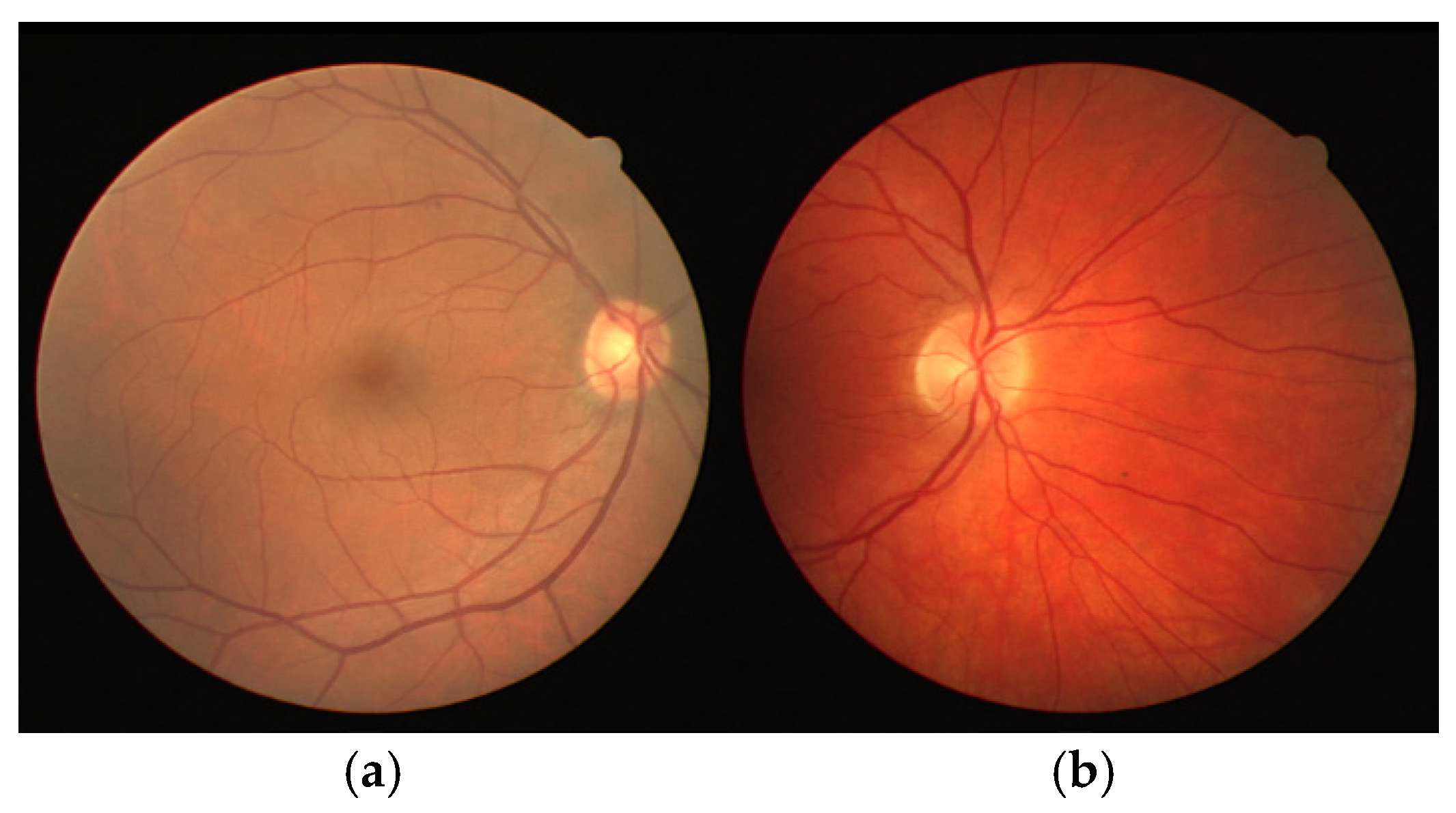
| DRIVE (Figure 1b) | TSA | - |
| AOA | TSA (3.50 × 10⁻³) | |
| SCA | TSA (2.4621 × 10⁻⁴) | |
| CSA | TSA (2.2337 × 10⁻⁵) AOA (4.1790 × 10⁻⁴) SCA (2.2337 × 10⁻⁵) | |
| GNDO | TSA (1.8307 × 10⁻⁵) AOA (3.6315 × 10⁻⁴) SCA (1.8307 × 10⁻⁵) | |
| GOBC-PA | TSA (1.0269 × 10⁻⁵) AOA (2.4155 × 10⁻⁴) SCA (1.0269 × 10⁻⁵) | |
| STARE (Figure 2a) | TSA | - |
| AOA | - | |
| SCA | TSA (1.2335 × 10⁻⁴) AOA (1.70 × 10⁻³) | |
| CSA | TSA (2.2337 × 10⁻⁵) AOA (4.1790 × 10⁻⁴) SCA (2.2337 × 10⁻⁵) | |
| GNDO | TSA (1.4191 × 10⁻⁵) AOA (3.0345 × 10⁻⁴) SCA (1.4191 × 10⁻⁵) | |
| GOBC-PA | TSA (1.0269 × 10⁻⁵) AOA (2.4155 × 10⁻⁴) SCA (1.0269 × 10⁻⁵) |
| DRIVE (Figure 1b) | STARE (Figure 2a) | ||
|---|---|---|---|
| CSA | Minimum MSE | 0.6631 | 0.5953 |
| CPU Time (seconds) | 2.8103 | 3.4689 | |
| TSA | Minimum MSE | 0.7077 | 0.6189 |
| CPU Time (seconds) | 0.4152 | 0.4869 | |
| AOA | Minimum MSE | 0.6803 | 0.6138 |
| CPU Time (seconds) | 2.6651 | 3.4248 | |
| GNDO | Minimum MSE | 0.6576 | 0.5918 |
| CPU Time (seconds) | 5.2565 | 6.6776 | |
| GOBC-PA | Minimum MSE | 0.6562 | 0.5920 |
| CPU Time (seconds) | 6.4216 | 8.3765 | |
| SCA | Minimum MSE | 0.6687 | 0.5996 |
| CPU Time (seconds) | 2.6980 | 3.4260 |
| Elapsed Time for NFEs (seconds) | |||
|---|---|---|---|
| Algorithms | Total NFEs | DRIVE (Figure 1b) | STARE (Figure 2a) |
| CSA | 1010 | 2.1720 s (77.28% of the total CPU time) | 2.6960 s (77.72% of the total CPU time) |
| TSA | 110 | 0.2820 s (67.92% of the total CPU time) | 0.3440 s (70.64% of the total CPU time) |
| AOA | 1010 | 2.0740 s (77.82% of the total CPU time) | 2.6720 s (78.02% of the total CPU time) |
| GNDO | 2000 | 3.9220 s (74.61% of the total CPU time) | 5.1320 s (76.85% of the total CPU time) |
| GOBC-PA | 2710 | 5.0150 s (78.09% of the total CPU time) | 6.5470 s (78.16% of the total CPU time) |
| SCA | 1010 | 2.0750 s (76.91% of the total CPU time) | 2.6120 s (77.20% of the total CPU time) |
Disclaimer/Publisher’s Note: The statements, opinions and data contained in all publications are solely those of the individual author(s) and contributor(s) and not of MDPI and/or the editor(s). MDPI and/or the editor(s) disclaim responsibility for any injury to people or property resulting from any ideas, methods, instructions or products referred to in the content. |
© 2025 by the authors. Licensee MDPI, Basel, Switzerland. This article is an open access article distributed under the terms and conditions of the Creative Commons Attribution (CC BY) license (https://creativecommons.org/licenses/by/4.0/).
Share and Cite
Çetinkaya, M.B.; Adige, S. Retinal Vessel Segmentation Using Math-Inspired Metaheuristic Algorithms. Appl. Sci. 2025, 15, 5693. https://doi.org/10.3390/app15105693
Çetinkaya MB, Adige S. Retinal Vessel Segmentation Using Math-Inspired Metaheuristic Algorithms. Applied Sciences. 2025; 15(10):5693. https://doi.org/10.3390/app15105693
Chicago/Turabian StyleÇetinkaya, Mehmet Bahadır, and Sevim Adige. 2025. "Retinal Vessel Segmentation Using Math-Inspired Metaheuristic Algorithms" Applied Sciences 15, no. 10: 5693. https://doi.org/10.3390/app15105693
APA StyleÇetinkaya, M. B., & Adige, S. (2025). Retinal Vessel Segmentation Using Math-Inspired Metaheuristic Algorithms. Applied Sciences, 15(10), 5693. https://doi.org/10.3390/app15105693