Stability-Preserving Model Reduction and Interpolation for Vibration Optimization in Beam-like Structures

Abstract

High-fidelity finite element models offer precise vibration analysis. However, their use in iterative optimization is computationally demanding. To overcome this, a stability-preserving framework for parametric model reduction and interpolation is developed. The interpolation approach is based on geometrically interpolating the poles of a system. As the scalar parameter varies, the poles follow specific trajectories, but their samples are only known at discrete points. Since the exact paths between these samples are unknown, a set of artificial trajectories is proposed. It is demonstrated that this set of trajectories guarantees stability and a bounded deviation in the H-infinite sense for multi-input multi-output linear time-invariant systems. Furthermore, all the trajectories that satisfy this bound are identified and presented. This approach introduces a new sampling criterion that assesses the parameter space sampling given on second-order models. In order to apply this criterion, a practical model order reduction strategy tailored to Bernoulli beam dynamics is presented. A numerical case study on a cantilever beam demonstrates the model order reduction method.

1. Introduction

In vibration analysis, ordinary differential equations are a powerful tool for modeling dynamic systems. However, accurate models often involve a large number of equations, which primarily aid in understanding complex physical phenomena. When used for simulation, control design, or vibration optimization, these models can be computationally inefficient and demand significant execution time and memory. To overcome this challenge, model order reduction techniques have been developed, creating reduced-order models that approximate the input-output behavior of large-scale systems with far fewer equations. Additionally, in engineering applications, system dynamics often depend on parameters such as material properties, geometry, or configuration. In such cases, parametric model order reduction (pMOR) [1] is necessary to account for these variations efficiently.

Generating and reducing large-scale models can be highly resource-intensive. For instance, a complex computational fluid dynamics (CFD) simulation [2,3] may take days to evaluate at a single value of the parameter. Similarly, optimizing a mechanical structure for vibration using the finite element method (FEM) often requires model evaluations at every step, even for systems with thousands of states. The primary objective of pMOR is to generate a reduced model that remains accurate for any parameter value, thus eliminating the need to repeat the modeling and reduction process.

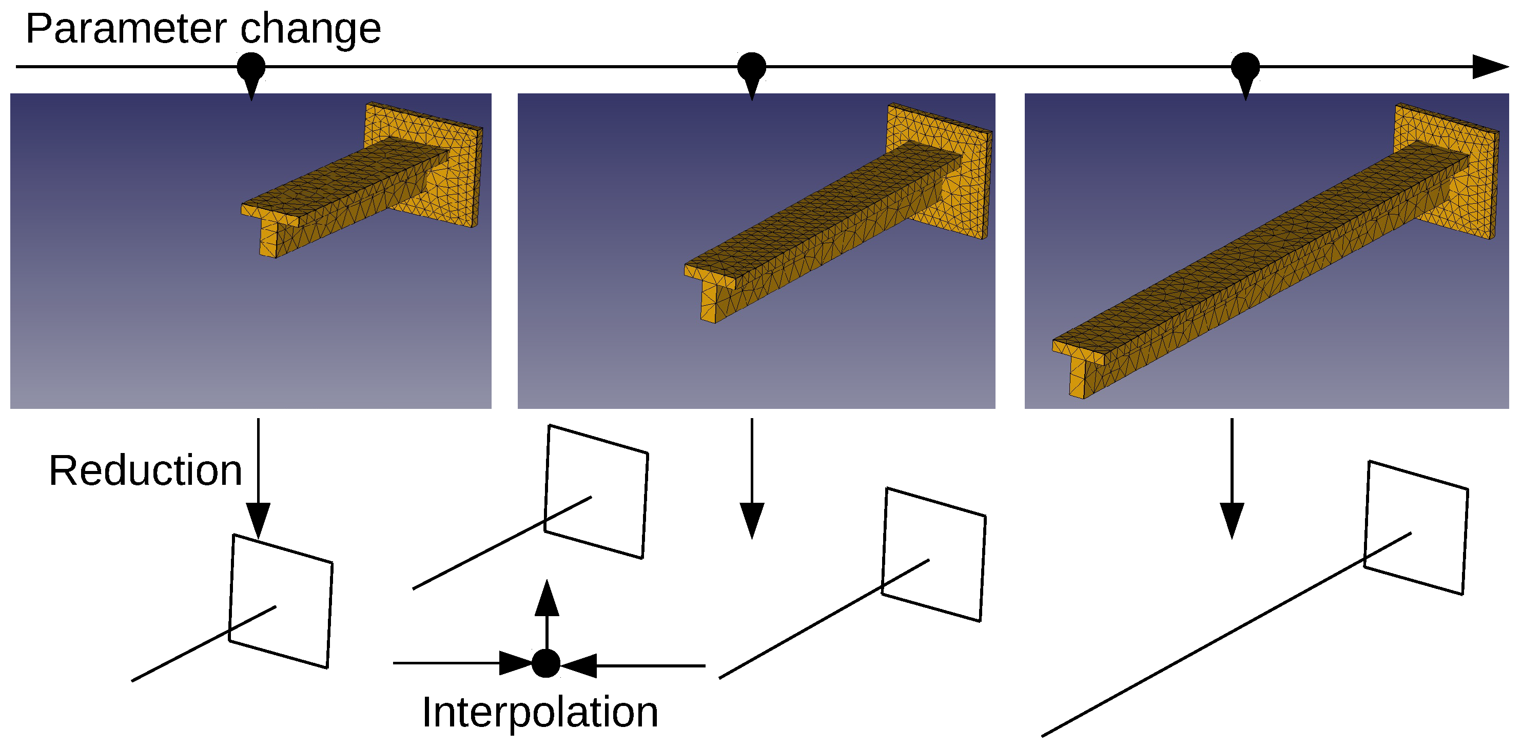
Typically, high-dimensional models that depend on parameters are only available at specific parameter values. As a result, most pMOR techniques leverage interpolation. The general approach of interpolation-based methods follows a two-step process: first, the high-dimensional models at selected parameter values are reduced independently. Then, reduced models for other parameter values are generated through interpolation using the existing reduced models ([4,5]); see Figure 1.

The figure represents a cantilever beam with varying lengths, which is treated as a parametric system. In this setup, reduced-order models are generated for different beam lengths. Once these reduced models are obtained, interpolation is performed between them to efficiently approximate the system’s behavior for new, unseen lengths, without needing to run a full simulation each time.

Because the behavior of the complex system at the desired parameter value is not directly known, additional prior information must be integrated into the interpolation algorithm. This ensures that the interpolated models closely capture the original behavior of the system beyond the initially available models. For instance, if the original system is known to be stable across the entire valid parameter domain, the interpolated system should also maintain stability.

Various pMOR techniques have been developed and applied to different classes of systems. Balanced truncation for parameter-dependent systems was explored in [6], which extends classical balanced truncation to parameter-dependent systems (including differential–algebraic equations) by computing reduced models on a set of parameter samples and constructing a single projection subspace valid for all parameters. This approach has a computationally expensive offline part and a much more efficient online part. Matrix interpolation techniques for local reduced order model (ROM) interpolation appeared in [7]. The study introduces a framework for parametric MOR via matrix interpolation. High-fidelity models are first reduced at various fixed parameter values, producing stable local ROMs. Then, the system matrices of these ROMs are interpolated across the parameter domain. This method ensures the interpolated ROM remains stable (using a matrix-measure criterion). Stability-preserving interpolation was comprehensively tackled in [1,8]. The papers propose an enhanced matrix-interpolation method that guarantees asymptotic stability of the parametric ROM. Here, each local ROM is post-processed via semidefinite programming to enforce strict dissipativity (passivity) so that it is stable. By interpolating these modified (dissipative) reduced models, the resulting parametric ROM remains stable for any intermediate parameter value. A data-driven Loewner framework for aeroelastic systems is introduced in [9]. The authors explore data-driven identification for parametric ROMs of aeroelastic systems. It uses a technique for modeling unsteady aerodynamic forces with parameter dependence. The approach employs the Loewner framework to fit parametric state-space models to frequency-domain data at multiple parameter settings, effectively interpolating transfer-function data into a reduced-order model. Optimization-based ${\mathcal{H}}_2\otimes {\mathcal{L}}_2$ reduction was advanced in [10]. The paper demonstrated that the ${\mathcal{H}}_2\otimes {\mathcal{L}}_2$ reduction framework extends to parametric LTI systems: first-order optimality conditions for structured ROMs were derived, and a stability-preserving optimization routine was devised, which yields locally optimal, stable reduced models with markedly lower errors at modest computational cost. Port-Hamiltonian structure preservation for pMOR was addressed by [11]. The study contributes a method aimed at preserving the inherent structure (e.g., port-Hamiltonian) of the original system in the reduced models. The approach integrates structure-preserving constraints into the MOR process so that the parametric ROM inherits properties like stability and passivity from the full-order model. Passivity-preserving reduction across parameter ranges was discussed in [12]. The authors focus on preserving physical system structure during parametric reduction. It introduces a pMOR technique that ensures the ROM remains passive (energy non-generating and stable) for all parameter values.

Another crucial aspect is ensuring that the interpolated model behaves similarly to the original high-order system. Since interpolation relies on information from a given set of reduced models, the parameter domain must be sampled densely enough to capture the system’s behavior accurately. More specifically, the combination of known models and a priori knowledge of the original system provides sufficient information to construct an interpolated model that closely resembles the original system from an application-specific perspective.

In most parametric LTI model interpolation, system evaluations are performed at selected parameter values, which serve as anchor points for interpolation. However, selecting these values is a non-trivial task. Poor choices can lead to significant errors, especially in regions with rapid system variation.

To improve accuracy, the samples should capture key changes in system behavior. Rather than distributing the points uniformly, methods like adaptive sampling and sensitivity analysis are used to place the samples where they are most informative [13,14]. These techniques propose an automated adaptive sampling strategy for parametric model order reduction (pMOR) using matrix interpolation, where the sampling points are chosen based on subspace distances in order to efficiently generate reduced models. The downside of these methods is that it is not evident how subspace distances translate to system behavior. In this regard, the paper presents a novel sampling criterion that links the criteria to the pole locations that can be interpreted easily by a trained user as system behavior.

An effective application of such algorithms is in optimizing drone structures. Enhancing unmanned aerial vehicle (UAV) design to minimize vibration improves flight stability, sensor accuracy, and component lifespan. In fixed-wing UAVs, it also helps mitigate flutter [15]. Drones are widely used in aerial surveying [16] and agriculture [17], but structural advancements can further enhance efficiency and durability. For multirotors, reducing frame resonance and motor-induced vibrations is as important as minimizing weight. Topology optimization [18,19] refines arm and hub structures to achieve an optimal stiffness-to-weight ratio. Fixed-wing UAVs prioritize reducing aeroelastic effects and engine-induced vibrations by optimizing wing and fuselage structure. Finite element analysis (FEA) and CFD provide accurate vibration predictions but require significant computational resources.

This paper builds upon the work presented in [20,21], which introduced a stability-preserving interpolation method for single-input single-output (SISO) linear time-invariant (LTI) systems with a scalar parameter.

In the case of a scalar parameter, the poles of the parametric LTI system move along a root locus or trajectory. However, for sampled systems, only discrete points along these loci are known. The key idea was to replace the unknown continuous trajectories with artificial ones between the sampled points, enabling interpolation along these constructed paths. It was shown that using hyperbolic lines as interpolating paths is particularly advantageous, as they preserve stability when the system is stable for all parameter values. Moreover, the interpolated system remains close to the original samples in the $H_{\infty }$ norm and, in certain cases, retains the minimum-phase property.

The problem with this approach is that one must connect the corresponding poles across different samples. However, in one sample, we have a distribution of poles, and in another sample, we have a different set of poles, with no apparent correspondence between them. To address this issue, the previous work solved an optimal matching problem based on the hyperbolic distance between the poles.

Other limitations of the previous work include that it only guarantees deviation bounds for SISO systems and restricts the pole trajectories to hyperbolic lines.

1.1. Contribution

A sampling criterion is developed to ensure proper pole matching for a certain class of second-order LTI systems. To meet this criterion, a practical model order reduction method is introduced, which is capable of handling structures that can be modeled using Bernoulli beam theory and which produces the required type of system. Examples of such beam-like structures include multicopter rotor arms and fixed-wing aircraft wings.

The method is extended to multiple-input multiple-output (MIMO) systems, and a corresponding deviation bound is also established.

The geometrical interpolation is generalized beyond hyperbolic lines, allowing for greater flexibility in the future. The set of all trajectories that satisfy the boundedness property is identified and presented.

1.2. Structure of the Paper

The remainder of this paper is organized as follows. Section 2 provides an in-depth discussion of the problem formulation, highlighting the key constraints. Section 3 introduces the proposed algorithm. Section 4 contains the proof for every bounded interpolating trajectory. Section 5 presents the proof for the MIMO extension. A short example is presented about the proposed model reduction method in Section 6.

2. Problem Formulation

In this paper, MIMO discrete time linear time-invariant systems are considered. Usually, the underlying phenomena that are examined are inherently continuous systems, but they can be sufficiently approximated with discrete time systems, and all the discussion is carried out with the assumption that the real system is modeled with a discrete system using appropriate sampling. Formally, let an element of the transfer function matrix be a generic transfer function [22]:

$$H(z,\zeta )={\displaystyle \frac{{\displaystyle \sum _{k=0}^m}{b}_k\left(\zeta \right)z^{-k}}{1+{\displaystyle \sum _{k=1}^n}{a}_k\left(\zeta \right)z^{-k}}}$$

(1)

where

• $\zeta \in \mathbb{R}$ is the parameter;
• $H(z,\zeta )$ is the transfer function at a certain $\zeta$ value;
• z is the complex variable of the function;
• $\left\{b_k\left(\zeta \right)\right\}$ are the numerator coefficients, where $b_k\left(\zeta \right)\in \mathbb{R}$;
• $\left\{a_k\left(\zeta \right)\right\}$ are the denominator coefficients, where $a_k\left(\zeta \right)\in \mathbb{R}$;
• m is the order of the numerator;
• n is the order of the denominator.

The following assumptions are made on $H(z,\zeta )$:

• The transfer function remains stable for all $\zeta$;
• It does not have any repeated poles;
• $m<n$, ensuring a proper transfer function;
• $\left\{b_k\left(\zeta \right)\right\}$ and $\left\{a_k\left(\zeta \right)\right\}$ are continuous function of $\zeta$;
• The sampling frequency is chosen to be high enough to ensure that all poles are mapped to the right-hand side of the complex plane while still remaining within the unit circle.

It is further assumed that for an element of the transfer function matrix that is $H(z,\zeta )$, there is a partial fractional expansion,

$$\begin{array}{c}\hfill H(z,\zeta )={\displaystyle \frac{r_1\left(\zeta \right)}{z-p_1\left(\zeta \right)}}+{\displaystyle \frac{r_2\left(\zeta \right)}{z-p_2\left(\zeta \right)}}+\dots +{\displaystyle \frac{r_n\left(\zeta \right)}{z-p_n\left(\zeta \right)}}\end{array}$$

(2)

where $p_i\left(\zeta \right)$ and $r_i\left(\zeta \right)$, for $i=1,\dots ,n$, represent the poles and residues.

The model $H(z,\zeta )$ is assumed to be difficult or impractical to evaluate for arbitrary values of $\zeta$. Instead, it is only available at k specific points, given by $G_i=H(z,{\zeta }_i)$ for $i=1,\dots ,k$. Consequently, the behavior of $H(z,\zeta )$ remains unknown for any $\zeta$ other than these given points.

Given that $\zeta$ is a scalar parameter, it is important to note that the models have a natural ordering. For instance, one can identify adjacent known models of $H(z,\zeta )$${\zeta }_i\le \zeta \le {\zeta }_{i+1}$ as $G_i$ and $G_{i+1}$. This ordering will be utilized in the following discussion.

This paper presents an interpolation algorithm that preserves stability and ensures that the deviation of the interpolated model from the known adjacent models remains within a guaranteed upper bound in terms of the $H_{\infty }$ norm. Formally, there exists a function f associated with the proposed interpolation method such that the following holds:

$$\begin{array}{cc}\hfill & {∥G\left(\zeta \right)-G_i∥}_{\infty }\le f(G_{i+1},G_i)\hfill \\ \hfill & {∥G\left(\zeta \right)-G_{i+1}∥}_{\infty }\le f(G_{i+1},G_i),{\zeta }_i\le \zeta \le {\zeta }_{i+1}\hfill \end{array}$$

(3)

where $G\left(\zeta \right)$ is the interpolated model. The derivation of f is presented in Section 4.

The proposed method is beneficial when it is known a priori that the given system remains stable for all parameter values and that the unknown function $H(z,\zeta )$, within the range ${\zeta }_i\le \zeta \le {\zeta }_{i+1}$, exhibits a behavior “similar” to $G_i$ and $G_{i+1}$. Such conditions frequently arise in practical applications. For instance, while the dynamics of an airplane vary with airspeed, it is known that the system remains stable within a certain speed range, and these dynamics change gradually. Similarly, geometrical modifications in a mechanical component often (though not always) result in predictable changes in its dynamic behavior. If the dynamics of the system are known for specific configurations, physical considerations suggest that other configurations will not exhibit arbitrary deviations. This problem formulation is conceptually similar to the one discussed in [20], but applied to individual elements of a transfer function matrix in a MIMO system. Since the interpolation is performed element-wise, this remains a valid approach.

2.1. Discussion on Assumptions

The requirement that $H(z,\zeta )$ remains stable for all $\zeta$ is very reasonable. In practical engineering, most systems are designed to operate stably across a range of parameter values. Many physical systems—such as electrical circuits, mechanical structures, and control systems—can be modeled this way, and stability under parametric variation is often a core design goal.

The assumption that $H(z,\zeta )$ has no repeated poles is moderately restrictive but still often realistic. In practice, repeated poles are uncommon in physical systems due to inherent damping and parameter variability. While idealized or overly simplified models may include repeated poles, most real-world systems do not. If this assumption is not met, the system may exhibit more complex transient behavior and be more sensitive to small changes in parameters, which complicates both analysis and implementation.

The condition $m<n$, ensuring a proper transfer function, is very standard and reflects the fact that real systems are causal and physically realizable. Nearly all real-world dynamic systems—across domains such as electronics, mechanics, and thermal processes—satisfy this assumption.

Lastly, the assumption that each element of $H(z,\zeta )$ admits a partial fraction expansion is common and reasonable. Most linear time-invariant systems with rational transfer functions can be expressed this way. If this assumption does not hold, it may indicate that the system is not described by a rational function, which limits the use of standard analytical and numerical tools in engineering practice.

Overall, these assumptions are not overly restrictive and align well with the characteristics of many real-world systems. They ensure that the model remains both mathematically tractable and physically meaningful.

2.2. Physical Meaning of the ${\mathcal{H}}_{\infty }$ Norm

The ${\mathcal{H}}_{\infty }$ norm of a stable LTI system quantifies the maximum gain from input to output across all frequencies. For a system with transfer function $G\left(s\right)$, physically, this means the system amplifies signals by at most ${\parallel G\parallel }_{\infty }$. This norm is especially important in robust control and filter design, as it reflects worst-case signal amplification. An application of this can be seen in [23].

2.3. Notations

Section 3 provides a detailed description of the algorithm. As demonstrated, $G\left(\zeta \right)$ for ${\zeta }_i\le \zeta \le {\zeta }_{i+1}$ is determined solely by $G_{i+1}$, $G_i$, and $\zeta$, meaning that only the adjacent models and the parameter $\zeta$ are utilized.

For convenience, the known models $G_{i+1}$ and $G_i$ are relabeled as $G_2$ and $G_1$, respectively. Accordingly, the jth pole of the $G_{i+1}$ model is denoted as $p_{j2}$, while the jth residual of $G_i$ is represented as $r_{j1}$.

Additionally, the parameter $\zeta$ is transformed into $\rho$ such that as $\zeta$ varies from ${\zeta }_i$ to ${\zeta }_{i+1}$, $\rho$ transitions from zero to one. The relationship between $\zeta$ and $\rho$ is given by the following:

$$\zeta =(1-\rho ){\zeta }_i+\rho {\zeta }_{i+1},\rho \in \{0,1\},i\in \{1,2,3,\dots \}.$$

(4)

Thus, the interpolated model is represented as $G\left(\rho \right)$ over the parameter range ${\zeta }_i\le \zeta \le {\zeta }_{i+1}$. The jth pole and residual of $G\left(\rho \right)$ are denoted as $p_j\left(\rho \right)$ and $r_j\left(\rho \right)$, respectively.

3. Interpolation Algorithm

The proposed algorithm is designed to interpolate between two adjacent models, $G_1$ and $G_2$. This section provides an overview of the algorithm, while its properties are analyzed in subsequent sections. The method incorporates certain aspects of hyperbolic geometry. In [24], Section 2 provides a concise overview of hyperbolic geometry fundamentals, also centered on the Poincaré disk model. This is expanded in Section 3, which uses a practical example to highlight how hyperbolic distance provides a proxy metric for comparing system dynamics. These foundations set the stage for exploring connections between hyperbolic metrics, system norms, and stability analysis. For further details, refer to [25,26].

In On the Correspondence of Hyperbolic Geometry and System Analysis [24], Section 2 provides a concise overview of hyperbolic geometry fundamentals, also centered on the Poincaré disk model. This is expanded in Section 3, which uses a practical example to highlight how hyperbolic distance provides a more accurate metric for comparing system dynamics than Euclidean distance. These foundations set the stage for exploring connections between hyperbolic metrics, system norms, and stability analysis.

The fundamental idea is that as the parameter varies, the poles of the model follow specific trajectories in the complex plane. However, since the model is only known at certain discrete points, only sampled positions of these pole trajectories are available. An interpolation approach can therefore involve replacing the original trajectories with artificial ones that connect the known points. A crucial aspect of this strategy is ensuring that the selected artificial trajectories adhere to the system’s known a priori properties (see Section 2).

In the previous study [20], hyperbolic lines were proposed as artificial trajectories connecting known samples. This choice was made because it preserves stability and provides a guaranteed upper bound on the deviation from the known models. In this paper, all of the possible trajectories that satisfy this condition are presented, paving the way for incorporating prior knowledge into the root loci if a particular problem is given. For further discussion, the hyperbolic line remains as a particular example because in a later section, Section 4, it serves as a reference for generalization.

The input data of the algorithm consist of static finite element method (FEM) data related to the structure at the two extreme ends of the parameter range. This means that the FEM model provides information about displacements regarding a certain load that is discussed later, at the minimum and maximum values of a given parameter.

3.1. Overview of the Algorithm

• Model reduction

  (a)

  From the FEM data a Bernoulli beam models are generated.

  (b)

  The beam models are discretized and second-order differential equations are generated.

• The natural frequency sensitivity is evaluated to assess the quality of the system’s sampling.
• The transfer function is generated in partial fractional form.
• The interpolated transfer function is constructed.

The first step is not a standard approach to reduce a high fidelity FEM model. The usual approach is to make a modal analysis in FEM and then using model reduction methods the reduced model is generated. As it will be discussed later, the standard model reduction methods are not suitable tools for the presented interpolation method, because the reduced model has to be in a certain form (details below), and most of the techniques cannot guarantee that. In the following, a detailed algorithm is introduced. The rationale for each step and the reasoning behind the chosen method are provided after the relevant information has been presented. The high level flowchart is in Figure 2. The steps of the algorithm are detailed in the following sections:

3.2. Model Reduction

Creating Bernoulli Beam Model

Create a high-fidelity finite element model of the structure under investigation. Subject the structure to a pure bending and evaluate the resulting distortion using finite element analysis (FEA) software. Subsequently, calculate the flexural stiffness based on the observed distortion. This process mirrors the approach taken when analyzing a real beam-like structure to determine its structural properties, as described in [27], but here, the physical scenario is replicated within an FEA environment.

The following are assumed:

• The structure can be modeled by a Bernoulli beam.
• Regarding the Bernoulli beam, the following is assumed:

  –

  Cross sections of the beam do not deform in a significant manner under the application of transverse or axial loads and can be assumed as rigid.

  –

  During deformation, the cross-section of the beam is assumed to remain planar and normal to the deformed axis of the beam.

• There is no bending–torsion coupling.
• The structure can be modeled as a beam in which all the principal axes of the cross-sections of the beam are parallel.
• The load is transferred to the structure using a rigid endplate, see Figure 3.
• For flexural stiffness determination, pure bending acts on the structure, which is created by equal and opposing forces, and the deflections (i.e., node displacements) are readily available from FEA software.

3.3. Discussion on the Physical Meaning and Scope of Applicability of the Assumptions

The structure is modeled as a Bernoulli beam. This theory assumes that transverse shear deformations are negligible, which is appropriate for slender beams where the length is significantly greater than the cross-sectional dimensions. It is particularly suitable when bending dominates the response, and shear effects do not contribute appreciably to the overall deformation.

Within this modeling framework, further assumptions are made regarding the behavior of the beam’s cross-sections. First, it is assumed that the cross-sections do not undergo significant deformation under applied loads and can be considered rigid. This means the shape and size of the cross-section remain essentially unchanged during loading, which is a valid assumption for beams made of stiff materials or with geometrically compact sections. Additionally, the cross-sections are assumed to remain planar and orthogonal to the deformed axis of the beam. This condition, central to Euler-Bernoulli theory, implies that no warping or shear distortion occurs and that the beam exhibits mostly pure bending deformation.

Another simplifying assumption is the absence of bending–torsion coupling. Physically, this means that the effects of torsion and bending can be treated independently, and one does not influence the other. This assumption holds when the cross-section is symmetric and loading is applied through the shear center, such that torsional and flexural responses are decoupled.

The model also assumes that all principal axes of the cross-sections remain parallel along the length of the beam. This implies a geometrically uniform or symmetrically varying beam without twist or out-of-plane curvature, ensuring that bending occurs consistently in the defined principal directions.

Finally, the last two assumptions are introduced to suit the subsequent calculations.

Here the used FEA software is Calculix Version 2.17 http://www.calculix.de/ (accessed on 9 January 2025) in combination with FreeCad CAD system version 1.0 https://www.freecadweb.org/ (accessed on 11 December 2024). All this software is free.

3.3.1. Calculating Flexural Stiffness

The theory behind this calculation is summarized as follows. Assume that the principal axes of the cross-sections of the beam under investigation are parallel. Choose a coordinate system regarding a beam in a way that the x-axis is parallel with the longitudinal axis of the beam, while one of the y or z-axis is parallel with one of the principal axes of the cross-section. For a Bernoulli beam, the following equation can be applied [28]:

$$v^{″}\left(x\right)=-{\displaystyle \frac{M_z\left(x\right)}{D\left(x\right)}}$$

(5)

where $D\left(x\right)$ is the flexural stiffness at the location x, $M_z\left(x\right)$ is the bending moment at location x and v is the displacement of the beam. The function $D\left(x\right)$ is often referred as $E\left(x\right)I\left(x\right)$, where $E\left(x\right)$ denotes the Young’s modulus at position x, and $I\left(x\right)$ is the second moment of area at that same point.

We know the displacement of the nodes of the FEM model and we know the bending moment at each cross-section, the aim is to calculate the $D\left(x\right)$ flexural stiffness function along the beam.

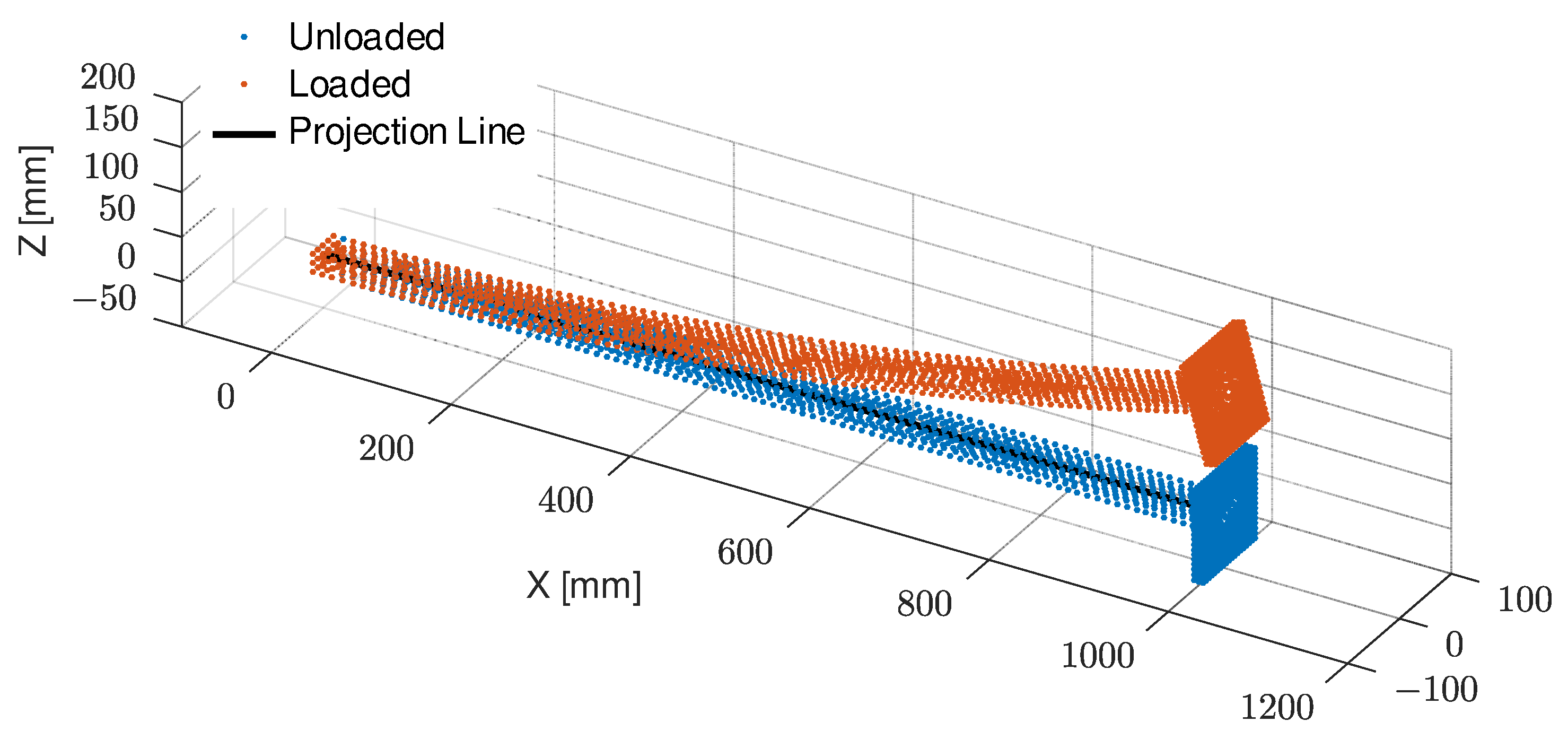
Next, the process of calculating flexural stiffness is presented. The basic approach is that we choose a line segment inside the point cloud of the nodes, and every node is projected onto that line segment. The line segment represents the neutral line, so it has to be chosen accordingly. The starting point of this line segment should be at the clamped end of the structure, while the other end should be at the other end of the structure. Now we define a coordinate system that has an x-axis that is collinear with the defined line segment, and the origin is at the clamped end of the structure, and it is directed to the other end of the projection line. The y axis of this coordinate system is perpendicular to the x axis. In this $x-y$ system, we can plot the projected node position versus node displacements, and a polynomial can be fitted to this set of data. To determine $D\left(x\right)$, the second derivative of the resultant polynomial is computed. It is worth noting that the precise selection of the projection line—ideally aligned with the neutral line—is beyond the current scope and is reserved for future work.

Step-by-step procedure:

• Translate the origin to the beginning of the projection line. The starting point of the projection line is $\underline{p_1}$ the endpoint is $\underline{p_2}$. Let the ith vector of a node be $\underline{n_i}=[n_{xi},n_{yi},n_{zi}]$. Then the ith translated node vector is $\underline{n_{ti}}=\underline{n_i}-\underline{p_1}$.
• Compute the unit vector of the projection line. Let the unit vector of the projection line be $\underline{p_u}$. So,

  $$\underline{p_u}={\displaystyle \frac{\underline{p_2}-\underline{p_1}}{{∥\underline{p_2}-\underline{p_1}∥}_2}}$$

  (6)
• Project the nodes to the projection line. Let the projected nodes be $\underline{n_p}$. Then,

  $$\underline{n_p}=\underline{\underline{n}}\underline{p_u}$$

  (7)

  where the $\underline{\underline{n}}$ matrix contains the coordinates of the nodes.
• Delete all the nodes that are outside the line segment. Every element of $\underline{n_p}$ is omitted if the element value is less than zero or greater than ${∥\underline{p_2}-\underline{p_1}∥}_2$.
• Compute the scalar displacements. There is a displacement vector associated with each node. In a bending load case, there is only one direction where the displacement is significant, so in order to avoid the introduction of a new coordinate frame, the length of the displacement vector is used. Let $\underline{\underline{d}}$ be the matrix of the coordinates of the displacements. The ith scalar displacement is $d_{si}={∥\underline{d_i}∥}_2$.
• Fit a polynomial to the $\underline{n_p}\to \underline{d_s}$ dataset. Since one end of the beam is clamped, the displacement and the first derivative of the displacement function at the clamping are zero because it is the boundary condition for the clamped constraint. Therefore, the zero-order and first-order terms in the fitted polynomial have to be zero. So the fitting is carried out as follows [29]:

  $$\underset{\underline{\underline{M}}}{\underbrace{\left[\begin{array}{cccc}{n}_{p1}^k& n_{p1}^{k-1}& \dots & n_{p1}^2\\ n_{p2}^k& n_{p2}^{k-1}& \dots & n_{p2}^2\\ ⋮& ⋮& \ddots & ⋮\\ n_{pN}^k& n_{pN}^{k-1}& \dots & n_{pN}^2\end{array}\right]}}\underset{\underline{\Theta }}{\underbrace{\left[\begin{array}{c}{a}_n\\ a_{n-1}\\ ⋮\\ a_2\end{array}\right]}}=\left[\begin{array}{c}{d}_{s1}\\ d_{s2}\\ ⋮\\ d_{sN}\end{array}\right]$$

  (8)

  where the $n_{pj}^k$ refer to the kth power of the x-coordinate of the jth projected point and $a_n\dots a_2$ are the coefficients of the polynomials.
  So the least-squares approximation of the polynomial parameters $\underline{\Theta }$ is as follows:

  $$\underline{\Theta }={\underline{\underline{M}}}^{+}\underline{d_s}$$

  (9)

  where “+” means pseudo-inverse that gives the least squares regression of the data [29].
• Differentiate the polynomial twice in order to obtain $v^{″}$.

3.3.2. Note on More Realistic Modeling

The main limitation of the above-described method is that it cannot handle bending–torsion coupling. One way to deal with this is that, in the bending case and the torsion case, ruled surface fitting is carried out. Since the approximating ruled surface is distorted and bent, a general method of ruled surface fitting should be applied, as in [30]. Bending–torsion coupling is significant in beam-like structures that are non-symmetric, composite, or curved. For example, slender curved beams or structures with off-axis material properties.

In such cases, bending in one direction causes twisting (torsion) and vice versa, due to geometry or material anisotropy.

Ruled surface fitting involves approximating a complex, often distorted or bent surface using a surface generated by sweeping a straight line along a spatial curve. This is useful for modeling deformations in beams, especially when they twist and bend, as it provides a geometrically intuitive way to approximate the shape changes.

3.4. Transfer Function Approximation of Bernoulli Beam

At this point, we have a differential equation that represents the Bernoulli beam model of the structure. A finite element model is generated from that model in the following form [28]:

$$\mathbf{M}\ddot{y}\left(t\right)+\mathbf{C}\dot{y}\left(t\right)+\mathbf{K}y\left(t\right)=0$$

(10)

• $\mathbf{M},\mathbf{C},\mathbf{K}\in {\mathbb{R}}^{N\times N}$ are the mass, damping, and stiffness matrices, respectively;
• $y\left(t\right)\in {\mathbb{R}}^N$ is the vector of generalized coordinates;
• $t\in {\mathbb{R}}^{+}$ denotes time.

It is important to note that this finite element model is a reduced version. Creating a finite element model from the Bernoulli beam model is a standard textbook exercise [31,32,33], so it is not detailed here. Note that for damping, we will use Rayleigh damping, but any diagonalizable damping is sufficient.

The important factor here is that the new model can contain the interpolation parameter $\rho$, which is not possible using ordinary FEM model. These parameters can be used to calculate the sensitivity of the natural frequency and, by extension, the sensitivity of the poles of the system. This is very important because if we can calculate the sensitivity of the poles regarding the parameters, then the sampling density of the interpolation parameter can be checked. For now, the process of sensitivity analysis is presented, and its importance will be discussed in the next steps of the algorithm.

The sensitivity analysis is based on [34]. The details can be found there. As is shown in [34],

$${\lambda }_{i,\zeta }={\lambda }_i{\displaystyle \frac{{\mathbf{u}}_i^T\left({\mathbf{K}}_{\zeta }-{\lambda }_i^2{\mathbf{M}}_{\zeta }+i{\lambda }_i{\mathbf{C}}_{\zeta }\right){\mathbf{u}}_i}{{\mathbf{u}}_i^T\left({\zeta }_i^2\mathbf{M}+\mathbf{K}\right){\mathbf{u}}_i}}$$

(11)

where

• ${\lambda }_{i,\zeta }={\displaystyle \frac{\partial {\lambda }_i}{\partial \zeta }}$ is the derivative of the ith eigenvalue with respect to $\zeta$;
• ${\lambda }_i$ is the ith natural frequency;
• ${\mathbf{M}}_{\zeta },{\mathbf{C}}_{\zeta },{\mathbf{K}}_{\zeta }$ are the derivative of the $\mathbf{M},\mathbf{C},\mathbf{K}$ with respect to $\zeta$;
• ${\mathbf{u}}_i$ are the mode shapes at specific parameter value.

At this point, it is obvious why it is important to have a model that contains the interpolation parameter. The matrices ${\mathbf{M}}_{\zeta },{\mathbf{C}}_{\zeta },{\mathbf{K}}_{\zeta }$ cannot be calculated otherwise.

Next, using this result, we show that a criterion can be given to the sampling of the interpolating parameter. If the criterion is met, then the sampling is good enough; if it is not, then finer sampling is required.

If $G_1=G_i$ corresponds to ${\zeta }_i$ and $G_2=G_{i+1}$ corresponds to ${\zeta }_{i+1}$, the jth pole $p_{j1}$ of the system $G_1$ is taken at ${\zeta }_i$, and the same pole $p_{j2}$ of the system $G_1$ is taken at ${\zeta }_{i+1}$, then it is easy to see that the position of the interpolated pole $p_{j\zeta }$ is in a circle:

$$p_{j\zeta }\in \{p_{j1}+t\left|(\zeta -{\zeta }_i){\lambda }_{j,\zeta }\right|e^{i\theta }:\forall t\in [0,1]and\forall \theta \in [0,2\pi )and{\zeta }_i\le \zeta \le {\zeta }_{i+1}\}$$

(12)

and similarly, if we take the estimation from the other end of the interpolating parameter:

$$p_{j\zeta }\in \{p_{j2}+t\left|({\zeta }_{i+1}-\zeta ){\lambda }_{j,\zeta }\right|e^{i\theta }:\forall t\in [0,1]and\forall \theta \in [0,2\pi )and{\zeta }_i\le \zeta \le {\zeta }_{i+1}\}$$

(13)

Let the circle around $p_{j1}$ when $\zeta ={\zeta }_{i+1}$ be $C_{j1}$ and the circle around $p_{j2}$ when $\zeta ={\zeta }_i$ be $C_{j2}$. So,

$$\begin{array}{cc}\hfill & C_{j1}=\{p_{j1}+t\left|({\zeta }_{i+1}-{\zeta }_i){\lambda }_{j,{\zeta }_i}\right|e^{i\theta }:\forall t\in [0,1]and\forall \theta \in [0,2\pi )\}\hfill \\ \hfill & C_{j2}=\{p_{j2}+t\left|({\zeta }_{i+1}-{\zeta }_i){\lambda }_{j,{\zeta }_{i+1}}\right|e^{i\theta }:\forall t\in [0,1]and\forall \theta \in [0,2\pi )\}\hfill \end{array}$$

Let

$$\mathcal{D}=\{D_j=C_{j1}\cup C_{j2}:j=1,2,3\dots n\},$$

(14)

where n is the number of poles. Each $D_j$ can either be connected or disjoint, depending solely on the properties of $C_{j1}$ and $C_{j2}$. From now on, we say $D_j$ is connected, meaning that $C_{j1}$ and $C_{j2}$ are overlapping.

Let

$$\mathcal{S}=\bigcup _{j=1}^n{D}_j$$

(15)

Notice that if all $D_j$ are connected, then $\mathcal{S}$ can contain at most n disconnected regions. These regions are the $D_j$, and they are formed by overlapping circles.

Now, we describe the sampling criteria of the system. As it is stated before, the interpolated poles must lie on an artificial trajectory between the end positions that are the samples of the system under examination. But it has to be known which pole corresponds to which pole. In [20], pole matching was used based on their hyperbolic distance, but it has no guarantee that the poles matched correctly. This is primarily due to the absence of an estimation for the fineness of sampling across the parameter range. Assuming that every $D_j$ is connected for any sampling, we can define the criterion:

Criterion 1.

If the set $\mathcal{S}$ on the complex plane contains exactly n disjoint subsets, then the pole matching problem is perfectly solved and the interpolating parameter sampling is sufficient, where n is the number of poles.

In other words, if every $D_j$ is connected and the sets satisfy $D_j\cap D_i=\varnothing$ for all $i\ne j$ (i.e., each compound set $D_j$, formed by a pair of circles, is disjoint from all others), then the sampling is fine enough.

In the following, we prove that if the circles $C_{j1}$ and $C_{j2}$ overlap for every sampling (i.e., all the $D_j$ are connected), then there exists a sampling that generates exactly n disjoint regions on $\mathcal{S}$.

Proof. 

Let $p_{j1}$ and $p_{j2}$ denote the jth pole at ${\zeta }_i$ and ${\zeta }_{i+1}$, respectively. Let ${\lambda }_{j,1}$ and ${\lambda }_{j,2}$ be the sensitivities of the jth pole at ${\zeta }_i$ and ${\zeta }_{i+1}$.

Given that

• the roots of a polynomial change continuously as its coefficients vary continuously;
• the sensitivity of the poles (see Equation (11)) is a continuous function of $\zeta$;
• the diameters of the circles $C_{j1}$ and $C_{j2}$ are continuous functions of $\zeta$, based on Equations (12) and (13)

the following limits hold:

$$\underset{\zeta \to {\zeta }_i}{\lim }{p}_{j\zeta }=p_{j1},\underset{\zeta \to {\zeta }_i}{\lim }{\lambda }_{j\zeta }={\lambda }_{j1}.$$

Here, $\zeta$ approaches ${\zeta }_i$ from the direction of ${\zeta }_{i+1}$.

The limit represents finer sampling, as increasingly finer discretization causes the poles and their sensitivities to become progressively closer.

Based on the limits above and Equation (12), the diameter of the circles $C_{j1}$ and $C_{j2}$ tends to zero as $\zeta$ approaches ${\zeta }_i$. Since no two poles can occupy the same location, there must exist a sampling such that all connected D regions are disjoined from each other. □

It follows that the regions $D_j,j=1,2,3\dots n$, formed by the union of overlapping circles corresponding to the same pole across sampled values of $\zeta$, vary continuously as well. Therefore, under sufficiently fine sampling, each $D_j$ remains connected, and disjointness between different D regions can be maintained, ensuring reliable pole matching.

Note that it does not matter whether we use hyperbolic or Euclidean geometry, since they have the same topology [25].

The intuition behind this is that the sensitivity of the poles determines their possible locations as the parameter varies from its initial to final value. Each pole must remain within a certain region—specifically, within a defined circle $C_{j1}$ at the starting value and within another circle $C_{j2}$ at the ending value of the parameter. This overlap indicates that the two different estimates are consistent. We assume the model does not vary so drastically that the region $D_j$ becomes disconnected. If all the overlapping pairs of circles are disjoint, then we have identified the correct pole matching. If this criterion is met, then the sampling of the system is sufficient; otherwise, the sampling needs to be finer.

3.5. Compute the Poles and the Residuals of $G_1$, $G_2$

This step is straightforward, given the assumption in Section 2 that the system admits a partial fraction decomposition.

3.6. Construct the Interpolated Transfer Function

As stated in [20], the formula for the interpolated transfer function, assuming a hyperbolic line between each corresponding pole and linear interpolation between residuals, is as follows:

$$H_{\rho }\left(z\right)=\sum _{i=1}^n{\displaystyle \frac{r_i\left(\rho \right)}{z-p_i\left(\rho \right)}}$$

(16)

where

$$p_i\left(\rho \right)={\displaystyle \frac{p_{i1}-\rho w_i}{1-\rho w_i\overline{p_{i1}}}}$$

(17)

$$r_i\left(\rho \right)=(1-\rho )r_{i1}+\rho r_{i2}$$

(18)

and

$$w_i={\displaystyle \frac{p_{i1}-p_{i2}}{1-p_{i2}\overline{p_{i1}}}}.$$

(19)

In (17), the parameter $\rho$ varies from 0 to 1. The formula used represents a parametrization of a hyperbolic line, for which we need to compute $w_i$ (see [26]). We can interpret it in a way that $\rho w_i$ is a straight line, not just in the hyperbolic sense, but also in the Euclidean sense, and that it is transformed using a congruent transformation to become the pole trajectory. This kind of transformation is always a Möbius transformation on the hyperbolic plane [26].

If we assume a general trajectory $t\left(\rho \right)$, then we can also use the same transformation, so we can write the following:

$$p_i\left(\rho \right)={\displaystyle \frac{p_{i1}-t\left(\rho \right)w_i}{1-t\left(\rho \right)w_i\overline{p_{i1}}}}.$$

(20)

The relevance of this type of construction is shown in the next section.

4. Boundedness and Stability

In earlier work, hyperbolic lines were proposed as artificial trajectories between known samples, owing to their stability-preserving nature and the existence of a guaranteed upper bound on the deviation from the known models. Since hyperbolic lines lie entirely within the unit circle, the poles of the interpolated system also remain inside the unit circle, ensuring system stability. In [20], these stability properties and deviation bounds are derived specifically for hyperbolic lines. Here, we extend the proof to cover all trajectories that satisfy the same bound.

The hyperbolic line, as an artificial pole trajectory, has favorable properties like stability preservation and uniform boundedness, but it never represents the behavior of the model and cannot be adapted to different situations. It is reasonable to assume that the locations of the poles follow some pattern as the parameter changes, and that is not a hyperbolic line. The interpolation method should be able to handle this additional information. In this section, the goal is to find a set of trajectories that have the same properties as the hyperbolic line. Using a larger set of trajectories enables techniques that adapt to specific pole trajectories.

Set of Bounded Trajectories

The hyperbolic line is stability preserving and satisfies the following deviation bound:

$$\begin{array}{cc}\hfill & {∥G\left(\rho \right)-G_1∥}_{\infty }\le f(G_1,G_2)=\max \{g_1(G_1,G_2),g_2(G_1,G_2)\}\hfill \\ \hfill & {∥G\left(\rho \right)-G_2∥}_{\infty }\le f(G_1,G_2)=\max \{g_1(G_1,G_2),g_2(G_1,G_2)\}\hfill \end{array}$$

(21)

where

$$\begin{array}{cc}\hfill & g_1(G_1,G_2)=\sum _{i=1}^n\left(\max \{\left|r_{i1}\right|,\left|r_{i2}\right|\}\max \left\{\left|{\displaystyle \frac{1}{1-\left|p_{i1}\right|}}\right|,\left|{\displaystyle \frac{1}{1-\left|p_{i2}\right|}}\right|\right\}+\left|{\displaystyle \frac{r_{i1}}{\frac{p_{i1}}{\left|p_{i1}\right|}-p_{i1}}}\right|\right)\hfill \\ \hfill & g_2(G_1,G_2)=\sum _{i=1}^n\left(\max \{\left|r_{i1}\right|,\left|r_{i2}\right|\}\max \left\{\left|{\displaystyle \frac{1}{1-\left|p_{i1}\right|}}\right|,\left|{\displaystyle \frac{1}{1-\left|p_{i2}\right|}}\right|\right\}+\left|{\displaystyle \frac{r_{i2}}{\frac{p_{i2}}{\left|p_{i2}\right|}-p_{i2}}}\right|\right).\hfill \end{array}$$

(22)

The detailed derivation can be found in [20]. In order to create a self-contained derivation, the first steps of the original derivation in [20] are repeated.

The rest of the section is devoted to the construction of a set that contains all the trajectories that satisfy Equation (21).

As assumed the systems $G\left(\rho \right)$ and $G_1$ have a partial fraction decomposition:

$${∥G\left(\rho \right)-G_1∥}_{\infty }={∥\sum _{i=1}^n\left(P_i\left(\rho \right)-P_{i1}\right)∥}_{\infty }$$

(23)

where

$$P_i\left(\rho \right)={\displaystyle \frac{r_i\left(\rho \right)}{z-p_i\left(\rho \right)}},P_{i1}={\displaystyle \frac{r_{i1}}{z-p_{i1}}}.$$

Exploiting the subadditivity of the $H_{\infty }$ norm from (23):

$${∥G\left(\rho \right)-G_1∥}_{\infty }\le \sum _{i=1}^n{∥P_i\left(\rho \right)-P_{i1}∥}_{\infty }$$

(24)

In the following, an upper bound is given on ${∥P_i\left(\rho \right)-P_{i1}∥}_{\infty }$.

$$\begin{array}{cc}\hfill & {∥P_i\left(\rho \right)-P_{i1}∥}_{\infty }={∥{\displaystyle \frac{r_i\left(\rho \right)}{z-p_i\left(\rho \right)}}-{\displaystyle \frac{r_{i1}}{z-p_{i1}}}∥}_{\infty }\le \hfill \\ \hfill & \left|r_i\left(\rho \right)\right|{∥{\displaystyle \frac{1}{z-p_i\left(\rho \right)}}∥}_{\infty }+{∥{\displaystyle \frac{r_{i1}}{z-p_{i1}}}∥}_{\infty }.\hfill \end{array}$$

(25)

Compute an upper bound term-by-term in (25). The last term can be calculated exactly since it is a first-order system:

$${∥{\displaystyle \frac{r_{i1}}{z-p_{i1}}}∥}_{\infty }=\underset{z=e^{i\omega }}{\max }\left|{\displaystyle \frac{r_{i1}}{z-p_{i1}}}\right|=\left|{\displaystyle \frac{r_{i1}}{\frac{p_{i1}}{\left|p_{i1}\right|}-p_{i1}}}\right|$$

(26)

The residual $r_i\left(\rho \right)$ in the first term is interpolated linearly:

$$\left|r_i\left(\rho \right)\right|=\left|(1-\rho )r_{i1}+\rho r_{i2}\right|\le \max \{\left|r_{i1}\right|,\left|r_{i2}\right|\}$$

(27)

The second term in (25) is also a first-order system like the last term, but it depends on $\rho$. As the first step, one can write:

$$\begin{array}{cc}\hfill & {∥{\displaystyle \frac{1}{z-p_i\left(\rho \right)}}∥}_{\infty }=\left|{\displaystyle \frac{1}{\frac{p_i\left(\rho \right)}{\left|p_i\left(\rho \right)\right|}-p_i\left(\rho \right)}}\right|=\left|{\displaystyle \frac{\left|p_i\left(\rho \right)\right|}{p_i\left(\rho \right)(1-\left|p_i\left(\rho \right)\right|)}}\right|={\displaystyle \frac{\left|p_i\left(\rho \right)\right|}{\left|p_i\left(\rho \right)\right|\left|(1-\left|p_i\left(\rho \right)\right|)\right|}}=\hfill \\ \hfill & {\displaystyle \frac{\left|p_i\left(\rho \right)\right|}{\left|p_i\left(\rho \right)\right|}}\left|{\displaystyle \frac{1}{1-\left|p_i\left(\rho \right)\right|}}\right|=\left|{\displaystyle \frac{1}{1-\left|p_i\left(\rho \right)\right|}}\right|=\left|{\displaystyle \frac{1}{1-\left|\frac{p_{i1}-\rho w_i}{1-\rho w_i\overline{p_{i1}}}\right|}}\right|.\hfill \end{array}$$

(28)

The expression

$$\left|{\displaystyle \frac{p_{i1}-\rho w_i}{1-\rho w_i\overline{p_{i1}}}}\right|\le 1$$

(29)

is less than or equal to one because it represents the pseudo-hyperbolic distance between the complex numbers $p_{i1}$ and $\rho w_i$ in the unit disk $\mathbb{D}$. Pseudo-hyperbolic distance is always less than or equal to one [25]. It is equal to one when one of the points is on the unit circle, which cannot happen since we assumed stable systems.

In order to construct an upper bound, the maximum of the expression

$$\underset{\rho }{\max }\left|{\displaystyle \frac{1}{1-\left|\frac{p_{i1}-\rho w_i}{1-\rho w_i\overline{p_{i1}}}\right|}}\right|$$

(30)

is needed. Since we discussed that the inner part $\left|{\displaystyle \frac{p_{i1}-\rho w_i}{1-\rho w_i\overline{p_{i1}}}}\right|$ is less than one, we can move the maximum operation inside the expression:

$$\underset{\rho }{\max }\left|{\displaystyle \frac{1}{1-\left|\frac{p_{i1}-\rho w_i}{1-\rho w_i\overline{p_{i1}}}\right|}}\right|=\left|{\displaystyle \frac{1}{{\displaystyle 1-\underset{\rho }{\max }\left|\frac{p_{i1}-\rho w_i}{1-\rho w_i\overline{p_{i1}}}\right|}}}\right|$$

(31)

A geometric approach is used to find the maximum of $\left|{\displaystyle \frac{p_{i1}-\rho w_i}{1-\rho w_i\overline{p_{i1}}}}\right|$ (see Figure 4). The term $\rho w_i$ traces a line segment from zero to $w_i$ (blue line), while $p_{i1}$ is a fixed point in the complex plane. The expression $\left|{\displaystyle \frac{p_{i1}-\rho w_i}{1-\rho w_i\overline{p_{i1}}}}\right|$ represents the pseudo-hyperbolic distance between $p_{i1}$ and any point along the segment defined by $\rho w_i$. A key geometric property states that the maximum distance between a fixed point and a point on a line segment occurs at one of the endpoints of the segment (these are depicted as a red line segment). Therefore, the maximum in (31) is reached when $\rho$ takes either of its extreme values, $\rho =0$ or $\rho =1$. As discussed in Section 3, the values of ${\displaystyle \frac{p_{i1}-\rho w_i}{1-\rho w_i\overline{p_{i1}}}}$ at $\rho =0$ and $\rho =1$ are $p_{i1}$ and $p_{i2}$ respectively:

$$\begin{array}{c}\hfill {∥{\displaystyle \frac{1}{z-p_i\left(\rho \right)}}∥}_{\infty }\le \max \left\{\left|{\displaystyle \frac{1}{1-\left|p_{i1}\right|}}\right|,\left|{\displaystyle \frac{1}{1-\left|p_{i2}\right|}}\right|\right\}\end{array}$$

(32)

It is worth noting that the result in (32) is connected to the choice of $w_i={\displaystyle \frac{p_{i1}-p_{i2}}{1-p_{i2}\overline{p_{i1}}}}$. $w_i$ is a point with the property that the hyperbolic distance of $w_i$ from the origin equals the hyperbolic distance between $p_{i1}$ and $p_{i2}$ and the hyperbolic distance of $w_i$ from $p_{i1}$ is equal to the hyperbolic distance between $p_{i2}$ and the origin. The distance of $w_i$ from the origin is a direct consequence of the definition of $w_i$.

After this, we can notice that the boundedness of the hyperbolic pole trajectory follows from the fact that the distance from a point to a line segment is maximal at one of the endpoints of the line segment see Figure 4.

In general, there is a set of curves that satisfy the condition that one of the endpoints is the furthest point from a given point in the plane. For example, see Figure 5. The furthest point on the line segment $\overline{w_{i}O}$ from $p_{i1}$ is $w_i$ in this example. The bound is determined by the furthest point, so every curve that starts from the origin O and ends at $w_i$ with no point on that curve having a distance from $p_{i1}$ which is greater than $d_h(p_{i1},w_i)$ gives the same bound. The geometric constraint is that any candidate curve must lie in the hyperbolic circle around $p_{i1}$ with radius $d_h(p_{i1},w_i)$ and must start from the origin and end at $w_i$.

It is obvious that the actual pole trajectory is obtained after the chosen $w_{i}O$ trajectory inside the boundary circle is transformed by Equation (20).

5. MIMO Extension

Let $H_{\rho }\left(z\right)$ be a transfer matrix. Each element of the matrix can be interpolated as an SISO system. For each element, there is an $H_{\infty }$ upper bound estimate; thus, using the Gerschgorin theorem, one can show that an upper bound estimate exists for the original system.

5.1. Maximal Singular Value Estimation Using Gerschgorin Theorem

Estimate the greatest singular value $\overline{\sigma }\left(A\right)$ of the matrix $A\in {\mathbb{C}}^{n\times m}$ using the Gerschgorin theorem. According to the Gershgorin Circle Theorem [35], every eigenvalue $\lambda$ of a matrix $A=\left[a_{ij}\right]\in {\mathbb{C}}^{n\times n}$ lies within at least one disk $D(a_{ii},R_i)$, where $R_i={\sum }_{j\ne i}\left|a_{ij}\right|$. Consider the matrix $A^{*}A$, where $A^{*}$ is the complex conjugate transpose of A since this matrix is positive semi-definite, all its eigenvalues are real. Thus, by definition $\overline{\sigma }\left(A\right)=\sqrt{{\lambda }_{\max }\left(A^{*}A\right)}$, where ${\lambda }_{\max }$ is the largest eigenvalue of $A^{*}A$.

Gerschgorin’s theorem provides an estimate on the location of the eigenvalues, so one can apply it to $A^{*}A$. Let $a_{ij}$ be an element of $A^{*}A$ and let the quantity $R_i$ be $R_i={\sum }_{j\ne i}\left|a_{ij}\right|$ sum of all non-diagonal elements in a row. A circle with center $a_{ii}$ and radius $R_i$ is called a Gerschgorin circle $D_i$. According to Gerschgorin’s theorem, the eigenvalues of $A^{*}A$ lie in one of the Gerschgorin circles. Since all the eigenvalues of $A^{*}A$ are real, the estimate of $\overline{\sigma }\left(A\right)$ is the largest point where a Gerschgorin circle intersects the real line.

Let $A\in {\mathbb{C}}^{n\times m}$ be a matrix. For the largest singular value $\overline{\sigma }$ of A the following holds:

$$\overline{\sigma }\left(A\right)\le \sqrt{\max \{D_i\cap \mathbb{R},i=1\dots rank\left(A^{*}A\right)\}}=\sqrt{\max \{R_i+a_{ii},i=1\dots rank\left(A^{*}A\right)\}}$$

(33)

where $D_i$ is the ith Gerschgorin circle of $A^{*}A$, $R_i$ is the radius of the ith Gerschgorin circle and $a_{ii}$ is the ith diagonal element of $A^{*}A$.

The inequality in (33) follows directly from the Gerschgorin theorem. The equality is true because the diagonal elements of $A^{*}A$ are positive reals, so the center points of the Gerschgorin circles lie on the real line, and the greatest value where one of the Gerschgorin circles intersects the real line is $\max \{R_i+a_{ii},i=1\dots rank\left(A^{*}A\right)\}$ It also means that

$$\overline{\sigma }\left(A\right)\le \sqrt{\max \left\{\sum _{j=1}^m\left|a_{ij}\right|,i=1\dots m\right\}}$$

(34)

where $a_{ij}$ is an element of $A^{*}A$.

5.2. Construction of Upper Bound for MIMO System

In this section, it is shown that the function f in (3) exists for a MIMO model if each element of the transfer matrix is interpolated piecewise as a SISO system. Thus, it is shown that a uniform bound can be given on the deviation of MIMO models $G\left(\rho \right)$ from $G_1$ in the following form:

$${∥G\left(\rho \right)-G_1∥}_{\infty }\le g_1(G_1,G_2).$$

(35)

The deviation of $G\left(\rho \right)$ from $G_2$ can be calculated analogously.

Let the transfer matrix of the system $G\left(\rho \right)-G_1$ be $M_{\rho }\left(z\right)$. The problem is to find an upper bound estimate on the $H_{\infty }$ norm of $M_{\rho }\left(z\right)$ that depends only on $G_1$ and $G_2$.

The $H_{\infty }$ norm of $M_{\rho }\left(z\right)$ at a given parameter $\rho$ is given by [36]:

$${∥G\left(\rho \right)-G_1∥}_{\infty }={∥M_{\rho }\left(z\right)∥}_{\infty }=\mathrm{ess}\underset{\omega \in \mathbb{R}}{\sup }\overline{\sigma }\left(M_{\rho }\left(e^{i\omega }\right)\right)$$

(36)

where $\overline{\sigma }\left(M_{\rho }\left(e^{i\omega }\right)\right)$ is the maximal singular value of the matrix $M_{\rho }\left(e^{i\omega }\right)$ at a given $\omega$. Every member of the studied class of systems (see Section 2) reaches its maximum on the unit circle. Therefore, there is no need for the essential supremum; a maximum can simply be used.

$${∥G\left(\rho \right)-G_1∥}_{\infty }={∥M_{\rho }\left(z\right)∥}_{\infty }=\underset{\omega \in \mathbb{R}}{\max }\overline{\sigma }\left(M_{\rho }\left(e^{i\omega }\right)\right)$$

(37)

The upper bound of the $H_{\infty }$ norm of $M_{\rho }\left(z\right)$ is

$${∥M_{\rho }\left(z\right)∥}_{\infty }\le \underset{\rho }{\max }{∥M_{\rho }\left(z\right)∥}_{\infty }=\underset{\rho }{\max }\underset{\omega \in \mathbb{R}}{\max }\overline{\sigma }\left(M_{\rho }\left(e^{i\omega }\right)\right)$$

(38)

Let ${\omega }_0$ and ${\rho }_0$ be the discrete frequency and parameter value where the maximal singular value of the matrix $M_{\rho }\left(e^{i\omega }\right)$ reaches its maximum. Let $m_{ij}\in \mathbb{C}$ be an element of the matrix $M_{{\rho }_0}\left(e^{i{\omega }_0}\right)$. Compute the Gerschgorin estimate ${\overline{\sigma }}^{\prime }$ of the maximal singular value $\overline{\sigma }$ of $M_{{\rho }_0}\left(e^{i{\omega }_0}\right)$. As the first step, the elements of $M_{{\rho }_0}^{*}\left(e^{i{\omega }_0}\right)M_{{\rho }_0}\left(e^{i{\omega }_0}\right)$ need to be expressed. Let $m_{ij}^{\prime }$ be an element of $M_{{\rho }_0}^{*}\left(e^{i{\omega }_0}\right)M_{{\rho }_0}\left(e^{i{\omega }_0}\right)\in {\mathbb{C}}^{n\times n}$ then:

$$m_{ij}^{\prime }=\sum _{k=1}^n\overline{m_{ki}}{m}_{kj}$$

(39)

where bar means complex conjugate. So the Gerschgorin estimate ${\overline{\sigma }}^{\prime }$ according to (34) is the following:

$${\overline{\sigma }}^{\prime }=\sqrt{\max \left\{\sum _{j=1}^n\left|m_{ij}^{\prime }\right|,i=1\dots n\right\}}=\sqrt{\max \left\{\sum _{j=1}^n\left|\sum _{k=1}^n\overline{m_{ki}}{m}_{kj}\right|,i=1\dots n\right\}}$$

(40)

we can move the absolute value operation inside the sum and apply it to each factor

$${\overline{\sigma }}^{\prime }=\sqrt{\max \left\{\sum _{j=1}^n\sum _{k=1}^n\left|\overline{m_{ki}}\right|\left|m_{kj}\right|,i=1\dots n\right\}}.$$

(41)

The value of ${\overline{\sigma }}^{\prime }$ is the Gersgorin estimate for ${\max }_{\rho }{\max }_{\omega \in \mathbb{R}}\overline{\sigma }\left(M_{\rho }\left(e^{i\omega }\right)\right)$. According to Equation (34), this estimate is greater than the upper bound of the $H_{\infty }$ norm of $M_{\rho }\left(z\right)$. That is,

$$\underset{\rho }{\max }\underset{\omega \in \mathbb{R}}{\max }\overline{\sigma }\left(M_{\rho }\left(e^{i\omega }\right)\right)\le {\overline{\sigma }}^{\prime }.$$

(42)

Notice that $\left|m_{ij}\right|$ is a value on the magnitude curve of a SISO transfer function at ${\omega }_0$ and ${\rho }_0$ on the unit circle. The transfer function is $G{\left({\rho }_0\right)}_{ij}-G_{1ij}$, following the definition of $M_{\rho }\left(z\right)$. The maximum of the magnitude curve of a SISO transfer function is equal to its $H_{\infty }$ norm. Therefore, $\left|m_{ij}\right|$ cannot exceed ${∥G{\left({\rho }_0\right)}_{ij}-G_{1ij}∥}_{\infty }$

$$\left|m_{ij}\right|\le {∥G{\left({\rho }_0\right)}_{ij}-G_{1ij}∥}_{\infty }\le f_{1ij}(G_{1ij},G_{2ij})$$

(43)

where the function $f_1$ is the upper bound estimate for a SISO system according to Section 4. The second inequality follows from the existence of the upper bound for SISO systems (see Section 4). Thus, from (41) and (43) the following is true:

$${\overline{\sigma }}^{\prime }=\sqrt{\max \left\{\sum _{j=1}^n\sum _{k=1}^n\left|\overline{m_{ki}}\right|\left|m_{kj}\right|,i=1\dots n\right\}}\le \sqrt{\max \left\{\sum _{j=1}^n\sum _{k=1}^n{f}_{1ki}{f}_{1kj},i=1\dots n\right\}}={\overline{\sigma }}^{″}$$

(44)

Thus, the upper bound for a MIMO system exists, and an estimate of it is ${\overline{\sigma }}^{″}$ since

$${∥G\left(\rho \right)-G_1∥}_{\infty }={∥M_{\rho }\left(z\right)∥}_{\infty }\le \underset{\rho }{\max }\underset{\omega \in \mathbb{R}}{\max }\overline{\sigma }\left(M_{\rho }\left(e^{i\omega }\right)\right)\le {\overline{\sigma }}^{\prime }\le {\overline{\sigma }}^{″}$$

(45)

6. Example

The interpolation and the usefulness in the optimization of this method are well documented in [20,21]. The example focuses on the construction of the Bernoulli beam model from FEM data.

We choose the simplest example in order to be able to verify the result using analytic calculations. Consider the massless cantilever beam that has a mass at the end (see Figure 6). This example is actually the building block of the lumped-mass FEM model of a Bernoulli beam therefore it can be easily extended to more complex cases.

The beam is an aluminum rod with a rectangular cross-section of 20 mm × 40 mm, with the following parameters:

• $L=$ 1 m
• $I=$ 26,666 ${\mathrm{mm}}^4$
• $E=$ 70 GPa
• $m=$ 1 kg

The applied load is a 0.1 Nm pure bending moment along the entire span. The unloaded nodes are projected onto the projection line (see Figure 7), then the corresponding displacement is carried to the next step.

In the next step, a polynomial is fitted to the projected data. Since the cross-section of the beam and the Young’s modulus of the material remain constant throughout, the solution to the Bernoulli equation is a quadratic polynomial [32]; therefore, a quadratic function is selected for the fitting process. However, in more general cases, the order of the polynomial must be selected carefully to obtain an acceptable result while avoiding overfitting. A higher-order polynomial may provide a closer fit to the data points, but it could also introduce artificial oscillations that do not reflect the true behavior of the system. Conversely, a lower-order polynomial might fail to capture important features.

In Figure 8, the node data and the fitted polynomial are nearly indistinguishable due to the accuracy of the polynomial fit. To provide insight into the deviation between the fitted polynomial and the original data, an additional plot displaying the error between these two datasets is included.

Since the fitted polynomial is a quadratic polynomial, its second derivative is a constant value given by $v^{″}=-5.3327\times {10}^{-5}$. Using Equation (5), the stiffness can be calculated as $I{E}_{FEM}=1875.2\mathrm{N}/\mathrm{m}$. The theoretical calculation gives $IE=\mathrm{26,666}\times {10}^{-12}\times 70\times {10}^9=1866.6\mathrm{N}/\mathrm{m}$, resulting in an error of less than one percent.

We now derive the transfer function of the beam, where the input is a force applied perpendicular to the tip, and the output is the resulting deflection of the beam.

The cantilever beam is modeled as a spring-mass-damper system with Rayleigh damping. The stiffness of a massless cantilever beam with modulus E, moment of inertia I, and length L is [28]:

$$k={\displaystyle \frac{3EI}{L^3}}.$$

(46)

Rayleigh damping is defined as follows [37]:

$$c=\alpha m+\beta k$$

(47)

where $\alpha$ is the mass-proportional damping coefficient, and $\beta$ is the stiffness-proportional damping coefficient.

The equation of motion for the mass m at the tip is the following:

$$m\ddot{x}\left(t\right)+c\dot{x}\left(t\right)+kx\left(t\right)=F\left(t\right).$$

(48)

Substituting $c=\alpha m+\beta k$,

$$m\ddot{x}\left(t\right)+(\alpha m+\beta k)\dot{x}\left(t\right)+kx\left(t\right)=F\left(t\right).$$

(49)

Taking the Laplace transform (assuming zero initial conditions),

$$m{s}^{2}X\left(s\right)+(\alpha m+\beta k)sX\left(s\right)+kX\left(s\right)=F\left(s\right).$$

(50)

Factoring $X\left(s\right)$,

$$X\left(s\right)\left[m{s}^2+(\alpha m+\beta k)s+k\right]=F\left(s\right).$$

(51)

The transfer function is

$$G\left(s\right)={\displaystyle \frac{X\left(s\right)}{F\left(s\right)}}={\displaystyle \frac{1}{m{s}^2+(\alpha m+\beta k)s+k}}.$$

(52)

After this point, the result expressed in [20,21] applies.

7. Conclusions and Future Work

In this paper, we presented a stability-preserving model reduction and interpolation method for optimizing the vibration characteristics of beam-like structures. The proposed approach integrates parametric model order reduction with an interpolation framework, which ensures stability and provides an upper bound on the deviation of interpolated models in the $H_{inf}$ norm. The method was extended to multiple-input multiple-output systems. Using geometric interpolation techniques within the hyperbolic plane, we constructed all possible interpolation trajectories that preserve the stability characteristics of the original system within this framework. Additionally, we introduced a criterion for assessing the adequacy of parameter sampling in the interpolation process, ensuring accurate pole matching.

The numerical example demonstrated the feasibility of deriving a reduced-order Bernoulli beam model from finite element method (FEM) data. The model’s accuracy was validated against theoretical calculations.

Several directions will be pursued to enhance the accuracy, robustness, and applicability of the proposed reduced-order modeling framework. A key focus will be on refining the interpolation strategy for residuals. In particular, the rationale behind the current use of linear interpolation will be critically examined, and alternative interpolation functions will be explored to more effectively capture the underlying system dynamics.

Further developments will also consider the extension of the methodology to accommodate vector-valued parameters, thus enabling the modeling of more complex structural variations. Additionally, incorporating higher-order sensitivity terms into the pole-matching process represents another promising direction to increase model fidelity.

Attention will also be directed toward the selection of the projection line, with a specific emphasis on its alignment with the neutral axis. Optimizing this aspect could yield improvements in the consistency and accuracy of the reduced models.

Another important area for future research involves the reduction of conservatism in the estimation of the maximum singular value for MIMO systems. While the Gerschgorin theorem provides a computationally efficient bound, it can result in overly conservative estimates. To address this, more precise techniques and specific estimation methods will be explored.

Moreover, the framework will be extended to rigorously analyze the propagation of approximation errors stemming from the polynomial fitting of deflection data.

Finally, the integration of previously established models, such as the Timoshenko beam model from [20,21], will be further explored. Given that this model adheres to the same second-order formulation as Equation (10), it can be seamlessly incorporated into the current framework. However, refinement of the reduction process remains necessary to fully leverage its potential.