
A Hybrid Deep Learning-Based Load Forecasting Model for Logical Range


Abstract
1. Introduction
- (1)
- We propose a domain-specific hybrid forecasting model tailored to the Logical Range context. Combining spatial and temporal representation learning through a GAF–CNN-SENet–GRU architecture, our approach effectively addresses the unique challenges of dynamic load behavior and distributed task execution observed in modern test and training infrastructures.
- (2)
- We design an innovative spatiotemporal attention fusion module that adaptively learns the significance of both spatial and temporal components in the data. This fusion mechanism enhances the model’s ability to generalize across diverse scenarios and operational conditions typically observed in Logical Range settings.
- (3)
- We conduct comprehensive experiments on real-world Logical Range datasets. The results demonstrate that our model outperforms state-of-the-art baselines in terms of accuracy, generalization, and robustness. Specifically, GCSG achieves an of 0.86, a mean absolute error (MAE) of 4.5, and a mean squared error (MSE) of 34, underscoring its practical utility in supporting more efficient and responsive resource scheduling across complex range systems.
2. Materials and Methods
2.1. Architecture for Logical Range
2.2. Proposed Load Forecasting Methodology
2.2.1. Spatial Feature Extraction
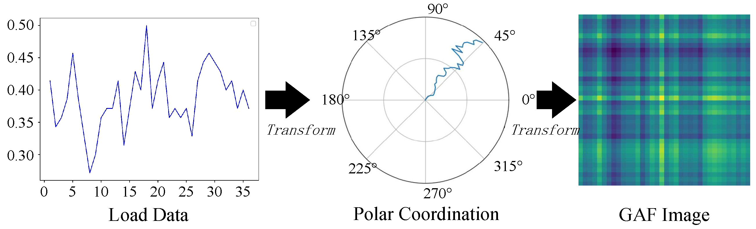
- Image conversion.
- (1)
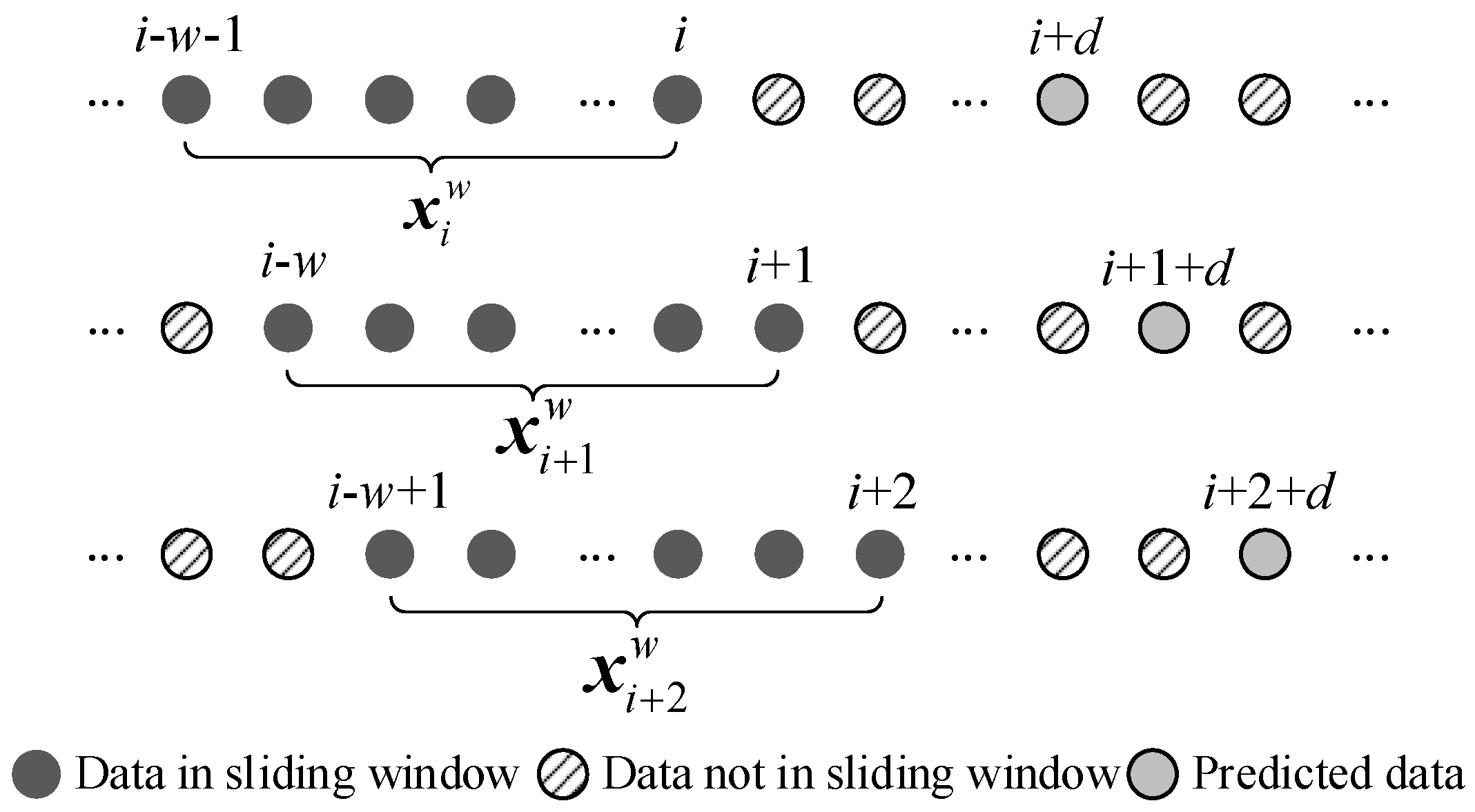
- Extract the input data from the dataset , where w is the length of and ;
- (2)
- Convert to polar coordinates using Equation (5):where is the polar radius, is the timestamp of , T is the total timestamp length, and is the polar angle. Here, preserves the temporal characteristics of the time-series data, while retains the numerical variations.
- (3)
- Construct the GAF matrix using the cosine function (Equation (6)), with dimensions :
- 2.
- Feature extraction.
- (1)
- Conduct successive convolution, activation, and pooling operations on to obtain feature maps , where the size of is and c is the number of channels, with each channel containing a two-dimensional feature.
- (2)
- Compute the global statistics for each channel feature in , where , using Equation (7):The global pooling operation aggregates the values of across its spatial dimensions to derive .
- (3)
- Compute the weight for each channel feature in to obtain the weight vector , where , using Equation (8):where denotes the sigmoid function, represents the ReLU function, and and are full layer matrices.
- (4)
- Compute the weighted feature map using Equation (9):
- (5)
- Apply convolutional and transformation operations on to obtain the spatial feature output vector for .
2.2.2. Temporal Feature Extraction
- (1)
- Input vector from dataset (where ) with initialized zero hidden state into the first GRU layer.
- (2)
- Compute reset gate, update gate, candidate hidden state, and hidden state updates using to obtain the hidden state vector .
- (3)
- Process and through the second GRU layer to generate the hidden state vector .
- (4)
- Transform via a fully connected layer to derive the temporal features output vector .
2.3. Feature Fusion
3. Results
3.1. Experimental Setup
3.2. Performance Evaluation Metrics
- The coefficient of determination () measures the proportion of variance in the predicted Logical Range load data explained by the model. Higher values indicate better performance:
- The mean absolute error (MAE) is computed as the average absolute difference between predicted and actual load forecasting values:
- The mean squared error (MSE) quantifies average squared prediction errors, penalizing larger deviations:
3.3. Performance Analysis
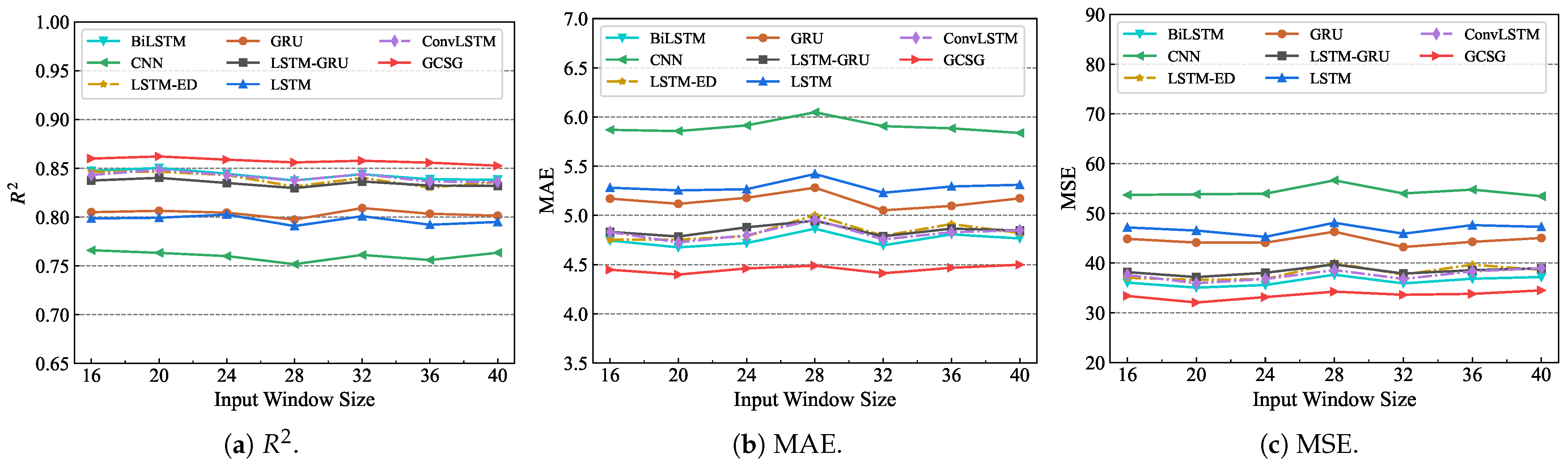
- (1)
- Input window size analysis.
- (2)
- Prediction step analysis.
3.3.1. Ablation Experiment
- GCSG: Full model (GAF+CNN+SENet+GRU).
- GCG: Ablated SENet (GAF+CNN+GRU).
- CSG: Ablated GAF (CNN+SENet+GRU).
- CG: Baseline (CNN+GRU).
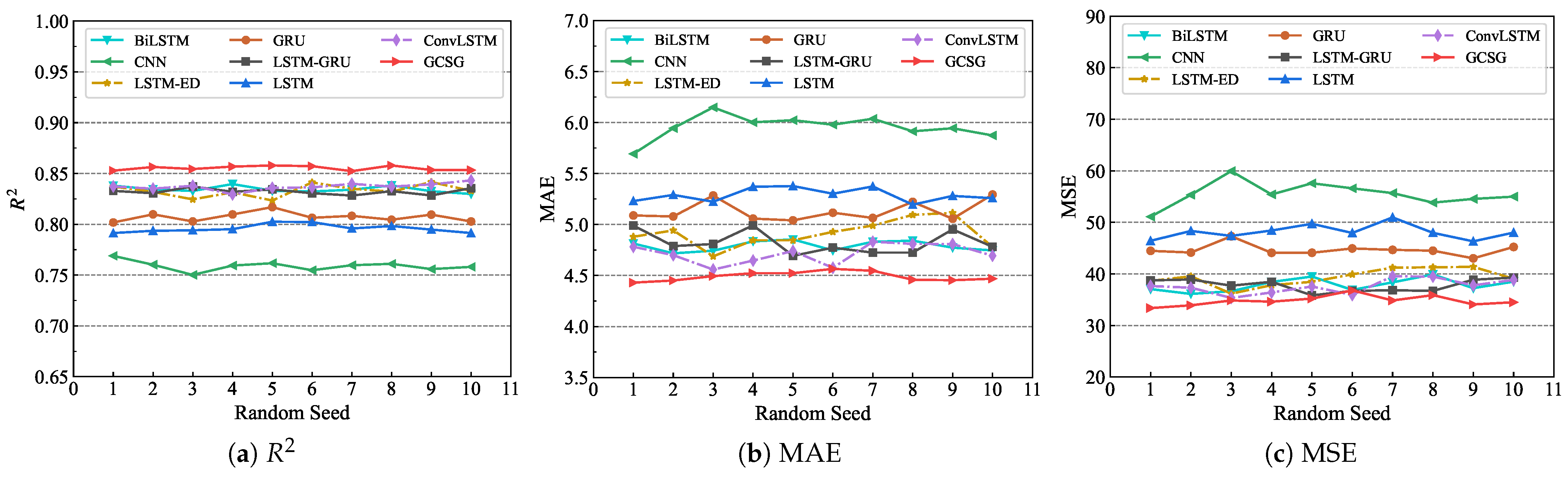
3.3.2. Generalization Performance
4. Discussion
5. Conclusions
Author Contributions
Funding
Data Availability Statement
Conflicts of Interest
References
- Chen, H.; Dang, Z.; Hei, X.; Wang, K. Design and application of logical range framework based on digital twin. Appl. Sci. 2023, 13, 6589. [Google Scholar] [CrossRef]
- Huan, M. Development of Logical Range Planning Furthermore, Verification Tool for Joint Test Platform. Master’s Thesis, Harbin Institute of Technology, Harbin, China, 2018. [Google Scholar]
- Li, D.; Li, L.; Jin, L.; Huang, G.; Wu, Q. Research of load forecasting and elastic resources scheduling of openstack platform based on time series. J. Chongqing Univ. Posts Telecommun. Nat. Sci. Ed. 2016, 28, 560–566. [Google Scholar]
- Khan, A.; Yan, X.; Tao, S.; Anerousis, N. Workload characterization and prediction in the cloud: A multiple time series approach. In Proceedings of the 2012 IEEE Network Operations and Management Symposium, Maui, HI, USA, 16–20 April 2012; pp. 1287–1294. [Google Scholar]
- He, J.; Hong, S.; Zhang, C.; Liu, Y.; Deng, F.; Yu, J. A method to cloud computing resources requirement prediction on saas application. In Proceedings of the 2021 International Conference on Machine Learning and Intelligent Systems Engineering (MLISE), Chongqing, China, 9–11 July 2021; pp. 107–116. [Google Scholar]
- Shyam, G.K.; Manvi, S.S. Virtual resource prediction in cloud environment: A bayesian approach. J. Netw. Comput. Appl. 2016, 65, 144–154. [Google Scholar] [CrossRef]
- Sun, W.; Zhang, H.; Palazoglu, A.; Singh, A.; Zhang, W.; Liu, S. Prediction of 24-hour-average PM2.5 concentrations using a hidden markov model with different emission distributions in northern california. Sci. Total Environ. 2013, 443, 93–103. [Google Scholar] [CrossRef] [PubMed]
- Dinda, P.A.; O’Hallaron, D.R. Host load prediction using linear models. Clust. Comput. 2000, 3, 265–280. [Google Scholar] [CrossRef]
- Liu, X.; Xie, X.; Guo, Q. Research on cloud computing load forecasting based on lstm-arima combined model. In Proceedings of the 2022 Tenth International Conference on Advanced Cloud and Big Data (CBD), Guilin, China, 4–5 November 2022; pp. 19–23. [Google Scholar]
- Mehdi, H.; Pooranian, Z.; Vinueza Naranjo, P.G. Cloud traffic prediction based on fuzzy arima model with low dependence on historical data. Trans. Emerg. Telecommun. Technol. 2022, 33, e3731. [Google Scholar] [CrossRef]
- Xie, Y.; Jin, M.; Zou, Z.; Xu, G.; Feng, D.; Liu, W.; Long, D. Real-time prediction of docker container resource load based on a hybrid model of arima and triple exponential smoothing. IEEE Trans. Cloud Comput. 2020, 10, 1386–1401. [Google Scholar] [CrossRef]
- Sharma, A.K.; Punj, P.; Kumar, N.; Das, A.K.; Kumar, A. Lifetime prediction of a hydraulic pump using arima model. Arab. J. Sci. Eng. 2024, 49, 1713–1725. [Google Scholar] [CrossRef]
- Prevost, J.J.; Nagothu, K.; Kelley, B.; Jamshidi, M. Prediction of cloud data center networks loads using stochastic and neural models. In Proceedings of the 2011 6th International Conference on System of Systems Engineering, Albuquerque, NM, USA, 27–30 June 2011; pp. 276–281. [Google Scholar]
- Karim, M.E.; Maswood, M.M.S.; Das, S.; Alharbi, A.G. Bhyprec: A novel bi-lstm based hybrid recurrent neural network model to predict the cpu workload of cloud virtual machine. IEEE Access 2021, 9, 131476–131495. [Google Scholar] [CrossRef]
- Shu, W.; Zeng, F.; Ling, Z.; Liu, J.; Lu, T.; Chen, G. Resource demand prediction of cloud workloads using an attention-based gru model. In Proceedings of the 2021 17th International Conference on Mobility, Sensing and Networking (MSN), Exeter, UK, 13–15 December 2021; pp. 428–437. [Google Scholar]
- Bi, J.; Ma, H.; Yuan, H.; Zhang, J. Accurate prediction of workloads and resources with multi-head attention and hybrid lstm for cloud data centers. IEEE Trans. Sustain. Comput. 2023, 8, 375–384. [Google Scholar] [CrossRef]
- Patel, E.; Kushwaha, D.S. A hybrid cnn-lstm model for predicting server load in cloud computing. J. Supercomput. 2022, 78, 1–30. [Google Scholar] [CrossRef]
- Kumar, J.; Goomer, R.; Singh, A.K. Long short term memory recurrent neural network (lstm-rnn) based workload forecasting model for cloud datacenters. Procedia Comput. Sci. 2018, 125, 676–682. [Google Scholar] [CrossRef]
- Rajagukguk, R.A.; Ramadhan, R.A.; Lee, H.-J. A review on deep learning models for forecasting time series data of solar irradiance and photovoltaic power. Energies 2020, 13, 6623. [Google Scholar] [CrossRef]
- Hu, J.; Shen, L.; Sun, G. Squeeze-and-excitation networks. In Proceedings of the IEEE Conference on Computer Vision and Pattern Recognition, Salt Lake City, UT, USA, 18–22 June 2018; pp. 7132–7141. [Google Scholar]
- Ilesanmi, A.E.; Ilesanmi, T.O. Methods for image denoising using convolutional neural network: A review. Complex Intell. Syst. 2021, 7, 2179–2198. [Google Scholar] [CrossRef]
- Woo, S.; Park, J.; Lee, J.-Y.; Kweon, I.S. Cbam: Convolutional block attention module. In Proceedings of the European Conference on Computer Vision (ECCV), Munich, Germany, 8–14 September 2018; pp. 3–19. [Google Scholar]
- Huang, J.; Ren, L.; Zhou, X.; Yan, K. An improved neural network based on senet for sleep stage classification. IEEE J. Biomed. Health Inform. 2022, 26, 4948–4956. [Google Scholar] [CrossRef] [PubMed]
- Cho, K.; Van Merriënboer, B.; Gulcehre, C.; Bahdanau, D.; Bougares, F.; Schwenk, H.; Bengio, Y. Learning phrase representations using rnn encoder-decoder for statistical machine translation. arXiv 2014, arXiv:1406.1078. [Google Scholar]
- Nguyen, H.M.; Kalra, G.; Kim, D. Host load prediction in cloud computing using long short-term memory encoder–decoder. J. Supercomput. 2019, 75, 7592–7605. [Google Scholar] [CrossRef]
- Zhang, M.; Wu, D.; Xue, R. Hourly prediction of PM2.5 concentration in beijing based on bi-lstm neural network. Multimed. Tools Appl. 2021, 80, 24455–24468. [Google Scholar] [CrossRef]
- Cho, M.; Kim, C.; Jung, K.; Jung, H. Water level prediction model applying a long short-term memory (lstm)–gated recurrent unit (gru) method for flood prediction. Water 2022, 14, 2221. [Google Scholar] [CrossRef]
- Shi, X.; Chen, Z.; Wang, H.; Yeung, D.-Y. Convolutional lstm network: A machine learning approach for precipitation nowcasting. Adv. Neural Inf. Process. Syst. 2015, 28, 1–9. [Google Scholar]


| Category | Specification |
|---|---|
| Operating system | Windows 10 (64-bit) |
| Programming language | Python 3.9 |
| Deep learning framework | PyTorch 2.0.0+ cu118 |
| Processor | 12th Gen Intel(R) Core(TM) i9-12900K 3.20 GHz |
| GPU | NVIDIA GeForce RTX 3090 |
| Memory | 64 (GB) |
| Model | Hidden Size | LR | Epochs | Batch Size | Dropout | Layers | Optimizer |
|---|---|---|---|---|---|---|---|
| CNN | 100 | 0.001 | 100 | 50 | 0.3 | 1 | Adam |
| LSTM | 10 | 0.1 | 50 | 50 | 0.3 | 1 | Adam |
| GRU | 64 | 0.001 | 50 | 50 | 0.3 | 1 | Adam |
| LSTM-ED | 64 | 0.0001 | 50 | 50 | 0.2 | 1 | Adam |
| BiLSTM | 10 | 0.01 | 50 | 50 | 0.01 | 1 | Adam |
| LSTM-GRU | 64 | 0.0001 | 50 | 50 | 0.4 | 1 | Adam |
| ConvLSTM | 64 | 0.001 | 50 | 50 | 0.01 | 1 | Adam |
| GCSG | 32 | 0.0001 | 100 | 100 | 0.01 | 2 | Adam |
| Parameter Category | Value/Range |
|---|---|
| Input window size (w) | (optimal ) |
| Prediction steps (d) | |
| Batch size | 100 |
| Training epochs | 2000 |
| Learning rate | 0.0001 |
| Optimizer | Adam |
| w | MAE | MSE | ||||||||||
|---|---|---|---|---|---|---|---|---|---|---|---|---|
| CG | GCG | CSG | GCSG | CG | GCG | CSG | GCSG | CG | GCG | CSG | GCSG | |
| 16 | 0.838 | 0.848 | 0.840 | 0.860 | 4.538 | 4.513 | 4.632 | 4.448 | 35.227 | 34.156 | 35.591 | 33.382 |
| 20 | 0.838 | 0.851 | 0.842 | 0.862 | 4.570 | 4.438 | 4.536 | 4.399 | 35.014 | 33.111 | 34.705 | 32.064 |
| 24 | 0.834 | 0.846 | 0.842 | 0.859 | 4.590 | 4.441 | 4.595 | 4.461 | 35.470 | 33.693 | 35.332 | 33.152 |
| 28 | 0.823 | 0.842 | 0.839 | 0.856 | 4.835 | 4.535 | 4.728 | 4.489 | 38.588 | 35.153 | 36.797 | 34.250 |
| 32 | 0.835 | 0.839 | 0.840 | 0.858 | 4.580 | 4.559 | 4.631 | 4.412 | 35.428 | 35.456 | 36.314 | 33.615 |
| 36 | 0.831 | 0.843 | 0.839 | 0.856 | 4.625 | 4.503 | 4.671 | 4.468 | 36.231 | 34.448 | 35.815 | 33.804 |
| 40 | 0.827 | 0.833 | 0.837 | 0.853 | 4.657 | 4.655 | 4.689 | 4.499 | 37.337 | 37.136 | 37.423 | 34.500 |
| d | MAE | MSE | ||||||||||
|---|---|---|---|---|---|---|---|---|---|---|---|---|
| CG | GCG | CSG | GCSG | CG | GCG | CSG | GCSG | CG | GCG | CSG | GCSG | |
| 1 | 0.831 | 0.843 | 0.838 | 0.855 | 4.900 | 4.556 | 4.722 | 4.450 | 38.282 | 35.631 | 37.529 | 33.827 |
| 3 | 0.784 | 0.801 | 0.792 | 0.803 | 5.520 | 5.346 | 5.435 | 5.303 | 51.475 | 46.546 | 49.793 | 45.259 |
| 5 | 0.768 | 0.782 | 0.778 | 0.791 | 5.690 | 5.518 | 5.655 | 5.438 | 53.305 | 50.533 | 52.345 | 49.243 |
| 7 | 0.755 | 0.770 | 0.763 | 0.773 | 5.822 | 5.598 | 5.744 | 5.548 | 55.901 | 52.717 | 54.334 | 51.084 |
| 9 | 0.746 | 0.763 | 0.753 | 0.770 | 5.966 | 5.705 | 5.910 | 5.627 | 58.975 | 53.928 | 57.096 | 52.407 |
| 11 | 0.743 | 0.758 | 0.752 | 0.764 | 6.138 | 5.819 | 6.034 | 5.783 | 60.000 | 56.050 | 58.238 | 55.400 |
| 13 | 0.738 | 0.752 | 0.746 | 0.759 | 6.258 | 6.045 | 6.171 | 5.894 | 63.843 | 59.929 | 61.346 | 58.356 |
| 15 | 0.731 | 0.751 | 0.741 | 0.754 | 6.300 | 6.109 | 6.222 | 5.991 | 64.941 | 61.575 | 63.057 | 59.696 |
| 17 | 0.721 | 0.746 | 0.733 | 0.751 | 6.389 | 6.184 | 6.281 | 6.128 | 65.950 | 62.054 | 64.927 | 60.328 |
| 19 | 0.709 | 0.740 | 0.717 | 0.746 | 6.537 | 6.299 | 6.450 | 6.227 | 68.927 | 62.948 | 67.559 | 60.916 |
| 21 | 0.704 | 0.730 | 0.713 | 0.740 | 6.639 | 6.321 | 6.562 | 6.265 | 70.981 | 63.918 | 68.213 | 62.744 |
| 23 | 0.692 | 0.726 | 0.701 | 0.730 | 6.686 | 6.355 | 6.599 | 6.283 | 72.933 | 65.966 | 71.213 | 64.096 |
| 25 | 0.689 | 0.722 | 0.696 | 0.728 | 6.711 | 6.406 | 6.637 | 6.307 | 73.829 | 66.748 | 72.583 | 65.703 |
| 27 | 0.687 | 0.714 | 0.695 | 0.723 | 6.832 | 6.490 | 6.749 | 6.407 | 74.894 | 67.993 | 73.312 | 66.731 |
| 29 | 0.668 | 0.694 | 0.672 | 0.703 | 7.162 | 6.698 | 7.017 | 6.634 | 79.975 | 74.379 | 78.637 | 73.266 |
Disclaimer/Publisher’s Note: The statements, opinions and data contained in all publications are solely those of the individual author(s) and contributor(s) and not of MDPI and/or the editor(s). MDPI and/or the editor(s) disclaim responsibility for any injury to people or property resulting from any ideas, methods, instructions or products referred to in the content. |
© 2025 by the authors. Licensee MDPI, Basel, Switzerland. This article is an open access article distributed under the terms and conditions of the Creative Commons Attribution (CC BY) license (https://creativecommons.org/licenses/by/4.0/).
Share and Cite
Chen, H.; Dang, Z. A Hybrid Deep Learning-Based Load Forecasting Model for Logical Range. Appl. Sci. 2025, 15, 5628. https://doi.org/10.3390/app15105628
Chen H, Dang Z. A Hybrid Deep Learning-Based Load Forecasting Model for Logical Range. Applied Sciences. 2025; 15(10):5628. https://doi.org/10.3390/app15105628
Chicago/Turabian StyleChen, Hao, and Zheng Dang. 2025. "A Hybrid Deep Learning-Based Load Forecasting Model for Logical Range" Applied Sciences 15, no. 10: 5628. https://doi.org/10.3390/app15105628
APA StyleChen, H., & Dang, Z. (2025). A Hybrid Deep Learning-Based Load Forecasting Model for Logical Range. Applied Sciences, 15(10), 5628. https://doi.org/10.3390/app15105628