ChaMTeC: CHAnnel Mixing and TEmporal Convolution Network for Time-Series Anomaly Detection

Abstract

Time-series anomaly detection is a critical task in various domains, including industrial control systems, where the early detection of unusual patterns can prevent system failures and ensure operational reliability. This paper introduces ChaMTeC (CHAnnel Mixing and TEmporal Convolution Network), a novel deep learning framework designed for time-series anomaly detection. ChaMTeC integrates an inverted embedding strategy, multi-layer temporal encoding, and a Mean Squared Error (MSE)-based feedback mechanism with dynamic thresholding to enhance anomaly detection performance. The framework is particularly tailored for industrial environments, where anomalies are rare and often subtle, making detection challenging. We evaluate ChaMTeC on six publicly available datasets and a newly introduced dataset, WaterLog, which is specifically designed to reflect real-world industrial control system scenarios with reduced anomaly rates. The experimental results demonstrate that ChaMTeC outperforms state-of-the-art models, achieving superior performance in terms of F1-CPA (Coverage-based Point-Adjusted F1) scores. The WaterLog dataset, which has been made publicly available, provides a more realistic benchmark for evaluating anomaly detection systems in industrial settings, addressing the limitations of existing datasets that often contain frequent and densely packed anomalies. Our findings highlight the effectiveness of combining channel-mixing techniques with temporal convolutional networks and dynamic thresholding for detecting anomalies in complex industrial environments. The proposed framework offers a robust solution for real-time anomaly detection, contributing to the reliability and sustainability of critical infrastructure systems.

1. Introduction

The sequential and temporal nature of time-series data makes them an essential part of many fields, such as manufacturing, healthcare, finance, and environmental monitoring. To ensure system security, dependability, and efficiency, it is essential to be able to analyze and identify anomalies in time-series data. Data points that substantially deviate from expected patterns are called anomalies, sometimes known as outliers or deviants. These deviations frequently point to important events that could have serious operational or financial repercussions, such as sensor malfunctions, equipment failures, cyberattacks, fraudulent transactions, or other anomalous behaviors [1,2].

Industrial environments, especially vital infrastructures such as manufacturing facilities, energy grids, and water management systems, are among the most important places for anomaly detection to be used. These systems are made up of several linked devices that frequently function in intricate and changing environments. To guarantee seamless operations, avoid system failures, and reduce the risks associated with natural or human-made disruptions, these infrastructures must be continuously monitored and managed. However, conventional threshold-based monitoring methods, which depend on static limits or pre-established rules, frequently cannot keep up with the complexity and unpredictability of actual industrial processes. Adoption of more sophisticated, data-driven anomaly detection techniques is required due to the unpredictability of operational environments, the existence of noise in sensor readings, and the changing behavior of interconnected components.

The creation of a baseline that reflects typical operational behavior is a crucial first step in the detection of industrial anomalies. It is possible to identify deviations that might point to possible threats or failures by comprehending and simulating typical system behavior. Predictive maintenance techniques can be created by utilizing past trends and patterns to identify and fix anomalies before they become serious issues. This method increases the resilience of vital infrastructures, reduces downtime, and allocates resources optimally. However, the lack of labeled anomalous data is a fundamental problem in these systems. Industrial anomaly detection frequently suffers from a severe imbalance between normal and abnormal instances, in contrast to traditional machine learning tasks, where labeled datasets are plentiful.

It is challenging to build supervised learning models that rely on substantial amounts of labeled training data because anomalies in these systems are uncommon, unpredictable, and highly context-dependent. Researchers have been concentrating more on unsupervised and semi-supervised techniques that do not require explicit labels for anomalies because of the shortcomings of supervised learning in industrial anomaly detection.

Clustering [3] and density estimation [4] are two examples of unsupervised techniques that look for anomalies based on statistical characteristics or departures from learned distributions. In a similar vein, semi-supervised methods concentrate on simulating typical behavior and identifying departures from the learned models. Reconstruction and forecasting methods based on deep neural networks are a commonly used class of models for this purpose. Reconstruction-based models [5] identify anomalies based on their inability to be accurately reconstructed, while autoencoders or generative models are used to encode normal patterns. Conversely, forecasting-based approaches [6] identify deviations as possible anomalies and forecast future values based on past observations.

The ability to detect anomalies in time-series data has been further improved by recent developments in deep learning and representation learning. Contrastive representation learning is one promising method that has recently been used for time-series anomaly detection [7] and has gained popularity in computer vision tasks [8,9]. The goal of contrastive learning is to improve the robustness of anomaly detection models by developing feature embeddings that optimize the difference between similar and dissimilar instances. Furthermore, to improve accuracy and adaptability, hybrid models that combine several detection methods, such as forecasting and reconstruction, have been introduced [10,11].

Even with great advancements in this area, there are still a number of difficulties, especially when anomalies are not evenly distributed throughout a dataset. Instead of being frequent and widespread, anomalies are sparse and localized in many industrial applications. The efficacy of current models may be diminished by this non-uniformity, which may result in irregular anomaly scores and reconstruction errors. More adaptive and context-aware thresholding mechanisms must be developed because traditional thresholding techniques for anomaly detection frequently do not generalize across various operational conditions.

To address these limitations, this study introduces an MSE-based feedback mechanism within an architecture that integrates both channel and temporal processing layers. Our approach leverages convolutional operations to effectively capture temporal dependencies while employing a dynamic thresholding method to enhance anomaly detection performance across different methodologies. Unlike static thresholding approaches that apply fixed anomaly detection criteria, our proposed dynamic thresholding method adjusts to variations in data distributions, reducing false positives and improving detection accuracy. Furthermore, we evaluate our method against existing techniques to assess its effectiveness in mitigating false alarms and improving anomaly detection robustness.

The main contribution of this work is the introduction of an MSE-based feedback mechanism within an architecture that integrates both channel and temporal processing layers. In this design, convolution is utilized to capture temporal correlations effectively. The proposed dynamic thresholding method is not only applied within our architecture but also tested on existing methods from the literature to evaluate its effectiveness across different anomaly detection approaches. Additionally, we adapt the previously designed WaterLog dataset—originally developed for industrial control system security research—to the anomaly detection domain. The adapted dataset, WaterLog*, is now publicly available for academic use and serves as a valuable benchmark. Unlike many public datasets with frequent and densely packed anomalies, WaterLog* features sparse and isolated anomaly regions, closely reflecting real-world scenarios where anomalies are rare and localized. This makes it a more challenging and realistic benchmark for evaluating anomaly detection methods.

2. Literature Review

The field of time-series anomaly detection has seen significant advancements, with classical methods evolving to address diverse data characteristics. Traditional techniques such as time-series decomposition, clustering, and density estimation have provided robust solutions for identifying anomalies, particularly in data with distinct patterns or significant deviations from normal distributions. Notable examples include the Local Outlier Factor (LOF) [4], which identifies anomalies based on local density deviations, and the Deep Autoencoding Gaussian Mixture Model (DAGMM) [12], which leverages density estimation principles. These methods are particularly effective in scenarios where the underlying data distribution is good, allowing for the identification of deviant outliers.

Clustering-based methods often use the distance to the cluster center as an anomaly score. For instance, ITAD (Integrative Tensor-based Anomaly Detection) [13] employs tensor-based decomposition to model normal behavior patterns and utilizes clustering to group similar patterns. This approach not only enhances the detection of anomalies but also facilitates the understanding of the underlying structure of the data, which can be crucial for operational insights. Deep-SVDD [3] trains a neural network to map normal data instances close to a central point in the latent space, while IForest [14] isolates anomalies through a recursive partitioning process, randomly selecting features and split values. The iterative nature of IForest enables the efficient processing of high-dimensional data, making it suitable for complex time-series datasets.

Autoregressive models, which predict future values based on past observations, have also been widely used. With the rise of deep learning, recurrent neural networks (RNNs) and their variants, such as LSTM networks, have gained prominence for their ability to capture long-term dependencies and temporal patterns. CL-MPPCA [15], an extension of ARIMA, combines LSTM-based neural networks with probabilistic PCA (Principal Component Analysis) models to detect deviations between predicted and actual values. This hybrid approach provides a more detailed understanding of the data as it combines both temporal dynamics and probabilistic modeling.

Autoencoders, a class of neural networks designed for dimensionality reduction and feature learning, have also been extensively applied in anomaly detection. They consist of an encoder that maps input data to a lower-dimensional latent space and a decoder that reconstructs the data from this representation. Variational Autoencoders (VAEs) extend this framework by encoding inputs into distributions, typically Gaussian, and reconstructing data from these distributions. For example, LSTM-VAE [16] and its improved variants [17,18] have been applied to anomaly detection. The ability of VAEs to model uncertainty in the data representation makes them particularly suitable for scenarios where anomalies may not conform to a single distribution.

Rao [19] presents a comprehensive examination of dimension reduction techniques in time-series data through a novel framework called the Bi-Functional Autoencoder (BFAE) in their work. The paper identifies the limitations of existing methods, such as Functional Principal Component Analysis (FPCA) and standard Autoencoders, which typically rely on linear approximations and scalar representations, thus inadequately addressing the complex and nonlinear nature of real-world time-series data. The authors propose an innovative methodology that utilizes a nonlinear function-on-function approach by integrating a functional encoder and decoder to effectively capture dynamic temporal relationships. This is achieved through the deployment of continuous neurons that facilitate the transformation of functional inputs into a lower-dimensional latent space, preserving the functional nature of the data throughout the encoding and decoding processes. Furthermore, the optimization of BFAE relies on traditional gradient descent techniques combined with Fréchet derivatives, allowing for computations of functional gradients that are essential for training the model. In contrast to conventional sequential models such as Recurrent Neural Networks (RNNs) and Long Short-Term Memory networks (LSTMs) that operate with fixed parameters, the BFAE provides a more nuanced framework that accommodates feature effects that dynamically change over time intervals. Overall, this advancement in functional data analysis presents promising applications across various domains, enabling improved efficiency and accuracy in the analysis of temporal data.

The article by Delibasoglu [20] presents LMS-AutoTSF, which distinguishes itself from traditional forecasting models by employing dual encoders that operate at multiple scales and is specifically designed to handle the nuanced variations in time-series data. These encoders utilize learnable filters to separate trend and seasonal components dynamically, employing both low-pass filters to capture long-term trends and high-pass filters for seasonal variations. This effectively allows the model to isolate and analyze the intricacies of the data in the frequency domain, a feature that is particularly beneficial for multivariate time-series forecasting, where different variables may interact and influence their temporal behaviors. The architecture integrates autocorrelation to enhance temporal modeling by computing lagged differences, thus capturing dependencies across time steps more efficiently than prior methodologies. Furthermore, the article elaborates on the challenges inherent in time-series forecasting, including the presence of linear and nonlinear trends, seasonal fluctuations, and the dynamic nature of the datasets, including those used for traffic forecasting (PEMS datasets) mentioned in the analysis. Traditional algorithms often struggle with these complexities; however, the LMS-AutoTSF framework combines frequency-domain filtering with temporal and channel-wise transformations, granting it an edge in discerning and processing detailed temporal patterns across multiple features and data dimensions. Consequently, this makes the model not only more effective in capturing long-term dependencies but also more efficient in processing, ensuring high precision while maintaining a lightweight design conducive to faster prediction times. The authors of [21] introduce an approach within the context of forecasting. Transformers have demonstrated significant capability in sequence modeling; however, they face scalability issues and performance degradation when dealing with multivariate series that include large lookback windows. The authors contend that standard Transformer architectures tend to merge multiple variables into single temporal tokens, impairing the model’s ability to learn meaningful representations and resulting in ineffective attention maps that fail to capture nuanced correlations. The proposed iTransformer architecture adopts an inverted approach, meaning that it separates the temporal and variable dimensions to enhance representation learning. The normalization process transforms individual variable representations into a Gaussian distribution, helping to mitigate inconsistencies caused by measurement discrepancies. This adjustment improves the model’s ability to effectively tackle non-stationary problems commonly found in time-series data. The authors utilize feed-forward networks (FFNs) customized for individual variable tokens, leveraging the universal approximation theorem to uncover complex relationships within the data. By doing so, the architecture efficiently encodes observed time-series data and decodes them for future predictions, demonstrating superior performance across seven real-world datasets compared with existing models such as Autoformer and LSTNet.

The authors of [22] introduce TimeMixer, a novel model designed for time-series forecasting that fundamentally utilizes a multiscale mixing approach. TimeMixer incorporates two primary architectural components: Past-Decomposable-Mixing (PDM) blocks and Future-Multipredictor-Mixing (FMM) blocks. The PDM blocks facilitate the decomposition of complex time series into distinct components such as seasonal and trend elements, allowing for fine-to-coarse and coarse-to-fine information mixing and effectively capturing both microscopic and macroscopic variations within the series. The FMM blocks, conversely, leverage multiple predictor models to enhance forecasting accuracy by exploiting complementary insights derived from varied temporal patterns across multiple scales. This method addresses the inherent challenges posed by the non-stationary nature of real-world data, which often exhibits intricate variations due to various influences, including trends and seasonal fluctuations common in applications ranging from economics to traffic planning. The empirical results demonstrate that TimeMixer achieves state-of-the-art performance across multiple benchmark datasets, thereby validating the efficacy of its proposed multiscale strategy in forecasting tasks.

The paper by Nie [23] investigates the efficacy of Transformer models for long-term forecasting within time-series data, particularly emphasizing advancements made possible through self-supervised learning techniques. The author gives details about the architecture of the proposed model, PatchTST, which leverages the capabilities of Transformers. Transformers are highlighted as suitable candidates for modeling sequential data due to their effective attention mechanisms, which facilitate learning relationships across broader contexts in data, unlike previous models. Additionally, the paper evaluates existing models, including state-of-the-art frameworks such as Informer, Autoformer, and FEDformer, establishing them as baselines to benchmark performance improvements achieved through the PatchTST architecture. The authors of [5] present a novel approach to unsupervised anomaly detection in time-series data by leveraging a Transformer-based architecture, which is referred to as the Anomaly Transformer. The central methodology involves adapting Transformer models that utilize self-attention mechanisms to capture intricate temporal dynamics and relationships within the time series. Key innovations include the introduction of an association-based criterion for anomaly identification, which is co-designed with temporal models to enhance the learning of informative associations across time points, thereby addressing limitations found in prior methodologies that primarily focused on pointwise or pairwise representations. The Anomaly Transformer demonstrates superior performance when benchmarked against various existing anomaly detection methods, including local outlier factors and clustering techniques, underscoring the importance of temporal information in accurately identifying anomalies in complex datasets. The comprehensive evaluation across multiple datasets further emphasizes the model’s robustness and generalizability, revealing a consistent state-of-the-art performance across benchmarks.

OmniAnomaly [17] integrates VAEs with a stochastic RNN (Recurrent Neural Network) framework using GRUs to model temporal dependencies, while InterFusion [24] employs a hierarchical VAE to capture inter-metric and temporal relationships. These developments highlight the importance of being able to identify both temporal and cross-metric relationships that can significantly increase the accuracy of anomaly detection in complex datasets. GAN-based methods, such as MAD-GAN [18] (Multivariate Anomaly Detection for time-series data with a Generative Adversarial Network), use LSTM networks in both the generator and discriminator to detect anomalies. The GANs training framework allows for the creation of realistic data distributions that can be used to effectively identify deviations.

DGHL [25] (Deep Generative model with Hierarchical Latent) introduces a hierarchical latent space representation using convolutional networks, enhancing the model’s ability to capture complex patterns in time-series data. This hierarchical approach allows for the modeling of both global and local patterns, which is essential for effective anomaly detection in multi-dimensional time series. BEATGAN [26] is another GAN-based reconstruction method. MTAD-GAT [10] combines forecasting and reconstruction-based networks, leveraging both outputs for anomaly detection. This dual approach not only enhances the robustness of the detection mechanism but also provides a comprehensive view of the data’s temporal dynamics.

Recent advancements have also introduced attention mechanisms into anomaly detection frameworks. AnomalyTransformer [5] introduces an Anomaly-Attention mechanism to compute association discrepancies, focusing on differences between normal and anomalous patterns. This attention mechanism allows the model to dynamically focus on the most relevant features of the data, improving the detection of subtle anomalies that may be overlooked by traditional methods. DCDetector [7] employs contrastive learning with a multi-scale dual attention model to enhance anomaly detection capabilities, demonstrating the effectiveness of attention-based approaches in this context. By leveraging contrastive learning, DCDetector can better differentiate between normal and anomalous patterns, leading to improved detection performance.

AE-FAR [27] (Autoencoder with Feedback Attention Reconstruction) integrates the capabilities of autoencoders and Recurrent Neural Networks (RNNs) with a feedback mechanism driven by reconstruction error. The method leverages autoencoders to learn compact representations of normal data and employs RNNs to capture temporal dependencies within time-series data. A key innovation of AE-FAR is its feedback mechanism, which utilizes the Mean Squared Error (MSE) to iteratively refine the reconstruction process. This iterative refinement process allows AE-FAR to adaptively improve its anomaly detection capabilities over time, making it particularly effective in dynamic environments where data characteristics may change.

As a result, advances in time-series anomaly detection reflect the rich interplay between classical methods and modern deep learning techniques. The integration of various methodologies, including clustering, density estimation, and advanced neural network architectures, has led to more robust and effective systems for identifying anomalies. As the field continues to evolve, ongoing research will likely focus on improving these methodologies and exploring new approaches to improve anomaly detection in complex time-series data. Future directions may include exploring hybrid models that combine the strengths of various techniques and applying transfer learning to improve performance in low-data scenarios.

3. Methodology

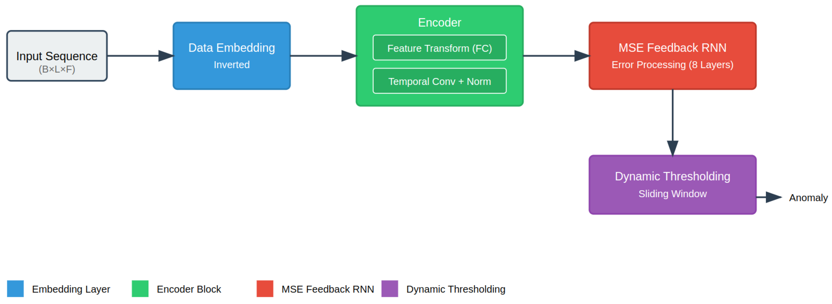
The anomaly detection process in our proposed ChaMTeC framework follows a systematic and modular pipeline that is designed to capture both temporal and feature-wise dependencies in multivariate time-series data. The process begins with input sequences $\mathbf{x}\in {\mathbb{R}}^{B\times L\times F}$, where B is the batch size, L is the sequence length, and F is the number of features (16 in our WaterLog dataset). The input is normalized and passed through the embedding layer called "DataEmbeddingInverted", which not only transforms feature dimensions but also prepares the data for temporal processing by transposing the sequence layout for improved temporal correlation learning. The core of the architecture consists of a multi-stage encoder composed of the following: feature-wise transformations using fully connected layers; a temporal self-attention module (optional) to capture long-range dependencies; a temporal convolutional module to extract localized temporal patterns; residual connections and layer normalization to stabilize training and enhance feature reuse. Once the embedding is encoded, a reconstruction of the original input is produced. The reconstruction error is computed as the Mean Squared Error (MSE), which serves as the basis for anomaly scoring. This error is then fed back into a Recurrent Neural Network (RNN), specifically, a GRU-based feedback mechanism, which adjusts the reconstruction iteratively by modeling the evolution of error patterns over time. The final corrected reconstruction is obtained by learning a residual correction from the RNN’s hidden states. To decide whether a sample is anomalous, we apply a sliding-window-based dynamic thresholding technique. This method calculates a moving average and standard deviation of error within a local window and computes a threshold. This allows the system to adapt to local variations and avoid false positives in high-variance but non-anomalous regions.

We propose a novel time-series anomaly detection framework that combines an inverted embedding strategy, channel (feature) fusion, multi-layer temporal encoding, and an MSE-based feedback mechanism with dynamic thresholding, as illustrated in Figure 1. The framework consists of four main components: (1) data embedding and input transformation (Section 3.1), which invert temporal and feature dimensions for temporal processing; (2) an encoder layer for temporal and feature processing (Section 3.2), which leverages both feature-wise transformations and convolutional temporal dependencies; (3) an MSE-based feedback recurrent neural network (Section 3.3), which iteratively refines reconstructions using squared error feedback; (4) sliding-window-based dynamic thresholding (Section 3.4.2), which adapts anomaly detection sensitivity to local data distributions.

3.1. Data Embedding and Input Transformation

The input sequence $\mathbf{x}\in {\mathbb{R}}^{B\times L\times F}$, where B is the batch size, L is the sequence length, and F is the feature dimension, is first processed using an embedding layer.

Let x denote the multivariate feature vector representing the operational state of the water management system. Each vector includes continuous measurements and indicators of all physical devices serving as data sources across five stations (tank, refilling1, refilling2, purification, and dam) working in the drinking water process. These features include variables such as the Dam Level, Purification Level, Elevator Level, Consumer Level, and Tank Level, as well as the pump status and flow level of these stations. The full feature vector spans n = 16 dimensions, and the data are collected at fixed intervals (e.g., 10 min), forming a multivariate time series used for anomaly detection.

DataEmbeddingInverted refers to the inverse transformation of input features with the aim of dimensionality transformation for temporal encoding. In our case, it denotes the reconstruction of the original input vector from its compressed representation, which is essential for reconstruction-based anomaly detection. This step typically involves a linear projection layer that maps low-dimensional latent vectors back to the input feature space.

$$\mathbf{z}=\mathrm{DataEmbeddingInverted}\left(\mathbf{x}\right)$$

(1)

where $\mathbf{z}\in {\mathbb{R}}^{B\times F\times D}$ represents the transformed embedding. This transformation ensures that the model captures temporal dependencies before further processing in the encoder.

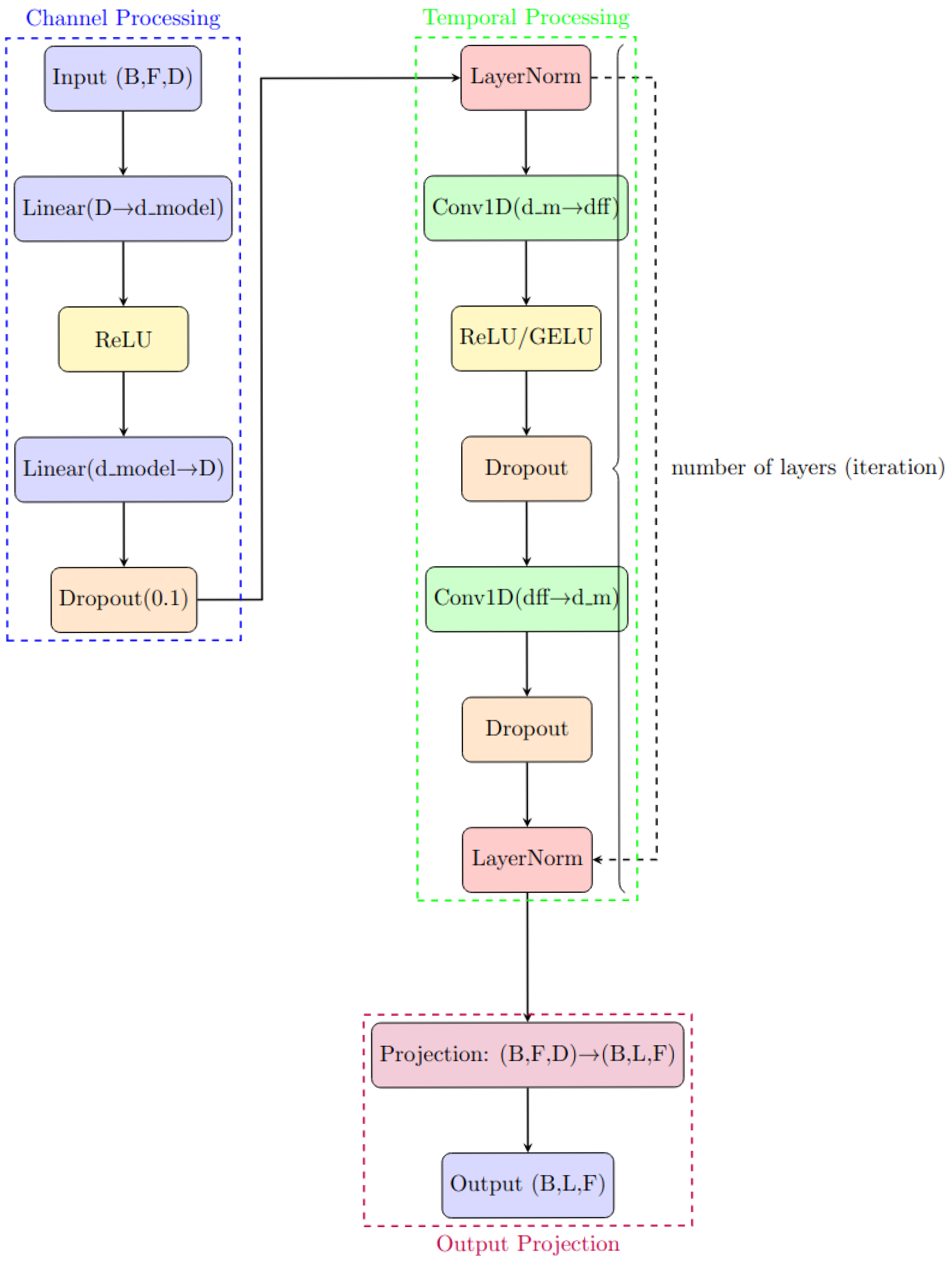
3.2. Encoder Layer for Channel and Temporal Processing

The encoder consists of multiple layers, each leveraging fully connected (FC) layers for feature-wise transformations and convolutional layers for temporal dependencies, as represented in Figure 2. This design enables the encoder to perform channel and temporal processing in a unified manner. Channel processing focuses on capturing the interactions between features (or sensor channels) at a given time step through fully connected layers, allowing the model to learn complex relationships such as correlations between pump flow, tank levels, and operational statuses. In parallel, temporal processing aims to model the evolution of each feature across time. To achieve this, the encoder integrates multi-head self-attention for learning long-range dependencies and dilated convolutional layers for capturing localized short-term trends. While attention enables the model to dynamically focus on relevant past time steps, convolutions ensure the efficient extraction of patterns across fixed-length receptive fields. Together, these mechanisms allow the encoder to simultaneously learn spatial (channel-wise) and temporal representations, making the framework robust against both point anomalies and context-dependent deviations in multivariate time-series data.

Multivariate time-series data in industrial systems exhibit dependencies both across features (channels) at each time step and along the temporal axis across sequences. Capturing these dependencies is essential for accurate anomaly detection. Therefore, the encoder is designed to jointly process. To achieve this, we implement a hybrid encoder that consists of two main stages:

• Channel Processing: Using fully connected (FC) layers applied to each time step independently, the encoder learns nonlinear transformations and inter-feature interactions in the input space. Feature embeddings are processed through a two-layer FC network as follows:

  $$\mathbf{h}=\sigma (\mathbf{z}{W}_1+b_1)$$

  (2)

  $${\mathbf{x}}^{\prime }=\mathrm{Dropout}(\mathbf{h}{W}_2+b_2)$$

  (3)

  where $W_1,W_2$ are the weight matrices, $b_1,b_2$ are biases, and $\sigma$ is the ReLU activation function. The dropout layer improves generalization.
• Temporal Processing: The encoder employs two complementary approaches for temporal modeling.
  Attention-based Temporal Processing: Multi-head self-attention captures global temporal dependencies. For input ${\mathbf{x}}^{\prime }$,

  $$\begin{array}{cc}\hfill \mathrm{MultiHead}\left({\mathbf{x}}^{\prime }\right)& =({\mathrm{head}}_1\parallel ,\dots ,\parallel {\mathrm{head}}_h)W_O\hfill \\ \hfill {\mathrm{head}}_i& =\mathrm{softmax}\left({\displaystyle \frac{\left({\mathbf{x}}^{\prime }{W}_Q^i\right){\left({\mathbf{x}}^{\prime }{W}_K^i\right)}^{\top }}{\sqrt{d_k}}}\right)\left(\mathbf{x}{W}_V^i\right)\hfill \end{array}$$

  (4)

  $${\mathbf{x}}_{\mathrm{attn}}=\mathrm{LayerNorm}(\mathbf{x}+\mathrm{Dropout}\left(\mathrm{MultiHead}\left(\mathbf{x}\right)\right))$$

  (5)
  Convolutional Temporal Processing: Local temporal patterns are captured through dilated convolutions as follows:

  $$\begin{array}{cc}\hfill \mathbf{y}& =\mathrm{ReLU}\left(\mathrm{Conv}1\mathrm{D}(\mathrm{LayerNorm}\left({\mathbf{x}}_{\mathrm{attn}}\right),W_c^1)\right)\hfill \\ \hfill {\mathbf{x}}_{\mathrm{conv}}& =\mathrm{LayerNorm}({\mathbf{x}}_{\mathrm{attn}}+\mathrm{Conv}1\mathrm{D}(\mathbf{y},W_c^2))\hfill \end{array}$$

  (6)

  where $W_c^1$ and $W_c^2$ are convolutional kernel weights. The normalization layer stabilizes training. The full encoder processes the input embedding through the following transformations:

  (a)

  Feature processing to the $d_{model}$ dimension;

  (b)

  Multi-head temporal attention;

  (c)

  Position-wise convolutional processing;

  (d)

  Layer normalization and residual connections.

  $${\mathbf{x}}_{\mathrm{enc}}=\mathrm{Encoder}\left(\mathbf{z}\right)=\mathrm{LayerNorm}(f_{conv}\left(f_{attn}\left(\mathbf{z}\right)\right)+\mathbf{z})$$

  (7)

  where $f_{attn}$ and $f_{conv}$ denote the attention and convolutional operations, respectively. This hybrid architecture combines the following:
  • Global receptive field via attention;
  • Local feature extraction via convolutions;
  • Stable training through residual connections.
  Mathematically, the encoder output is given by

  $${\mathbf{x}}_{\mathrm{enc}}=\mathrm{Encoder}\left(\mathbf{z}\right)$$

  (8)

  where ${\mathbf{x}}_{\mathrm{enc}}\in {\mathbb{R}}^{B\times F\times D}$ is the encoded representation used for subsequent forecasting and error feedback mechanisms. To align the encoded representation with the desired input dimensions for the reconstruction, a projection layer is applied. This layer transforms the representation from $B\times F\times D$ to $B\times L\times F$, ensuring compatibility with the subsequent processing steps.

This combination of global (attention) and local (convolutional) processing, together with residual connections and normalization, enables robust sequence encoding. It equips the model to detect both point anomalies (e.g., abrupt state changes) and contextual anomalies (e.g., gradual divergence from operational norms) within multivariate industrial data.

3.3. MSE-Based Feedback Recurrent Neural Network

To refine time-series reconstruction, we propose an MSE-based feedback recurrent neural network (MSEFeedbackRNN) that leverages squared reconstruction errors to iteratively improve predictions. This approach enables the model to dynamically adjust future predictions by learning error dependencies over time, as briefly represented in Figure 3.

RNN stands for Recurrent Neural Network, a type of deep learning model designed to process sequential data by maintaining a hidden state across time steps. In this study, we use RNNs to model the temporal dependencies in multivariate time-series data. Specifically, the RNN layer captures how the operational states of pumps, switches, and volume levels evolve over time. The MSEFeedbackRNN module is configured with an input size of the feature dimension, a hidden size of half the input size (8 for WaterLog), and an output size equal to the input size (16 for WaterLog). The model uses a multi-layer RNN architecture with 8 stacked recurrent layers, allowing it to capture hierarchical temporal dependencies. The recurrent layer is followed by a linear projection layer that maps the hidden-state outputs back to the original input dimensionality. All RNN computations are performed in batch-first mode to align with the input tensor format (batch, sequence, features).

3.3.1. Error Computation and Injection

Given an input sequence $\mathbf{x}\in {\mathbb{R}}^{B\times L\times F}$, the reconstructed output $\widehat{\mathbf{x}}$ is obtained from the output of the encoder module and the projection layer. The reconstruction error is computed as the following element-wise squared difference:

$$\mathbf{e}={(\mathbf{x}-\widehat{\mathbf{x}})}^2.$$

(9)

To propagate error information into future steps, the error sequence is injected into the reconstruction output as follows:

$${\mathbf{x}}_{\mathrm{feedback}}=\widehat{\mathbf{x}}+\mathbf{e}.$$

(10)

This formulation ensures that regions with higher reconstruction errors have a greater influence on the feedback process, enabling the model to focus on correcting large deviations.

3.3.2. Temporal Error Processing with RNNs

The error-augmented sequence ${\mathbf{x}}_{\mathbf{feedback}}$ is processed by a recurrent neural network (RNN) with H hidden units and D layers to capture temporal dependencies in the error dynamics as follows:

$${\mathbf{h}}_t=RNN({\mathbf{x}}_{\mathbf{feedback}},\mathbf{t},{\mathbf{h}}_{t-1}),$$

(11)

where ${\mathbf{h}}_t$ represents the hidden state at time step t, and $RNN(·)$ is the recurrent function, such as an RNN. The output of the RNN is then projected back to the original feature space as follows:

$$\mathbf{c}=W_o\mathbf{h}+b_o,$$

(12)

where $W_o\in {\mathbb{R}}^{H\times N}$ and $b_o\in {\mathbb{R}}^N$ are learnable parameters.

3.3.3. Final Correction and Reconstruction

The final reconstructed sequence is obtained by adding the learned correction $\mathbf{c}$ to the original reconstruction output as follows:

$$\widehat{{\mathbf{x}}_{\mathbf{final}}}=\widehat{\mathbf{x}}+\mathbf{c}.$$

(13)

This iterative feedback mechanism allows the model to refine predictions over multiple time steps, adapting to recurring error patterns and improving reconstruction quality. To ensure numerical stability, input sequences are first normalized using their mean and standard deviation as follows:

$$\tilde{\mathbf{x}}={\displaystyle \frac{\mathbf{x}-\mu }{\sigma }},$$

(14)

where $\mu$ and $\sigma$ are the mean and standard deviation computed along the sequence dimension. After reconstruction, denormalization is applied to restore the original scale as follows:

$$\widehat{{\mathbf{x}}_{\mathbf{final}}}=\widehat{{\mathbf{x}}_{\mathbf{final}}}·\sigma +\mu .$$

(15)

This step ensures that error adjustments remain meaningful in the original data domain.

3.4. Thresholding for Anomaly Detection

3.4.1. Static Thresholding for Anomaly Detection

Static thresholding is a widely used approach for anomaly detection, particularly in scenarios where the anomaly ratio is known or can be estimated. This method involves computing a fixed threshold based on the distribution of reconstruction errors (e.g., the Mean Squared Error or MSE) derived from the training data. The threshold is typically set as the $(100-\alpha )$-th percentile of the error distribution, where $\alpha$ represents the expected proportion of anomalies in the data. Formally, the threshold $\tau$ is defined as follows:

$$\tau =Q_{100-\alpha }\left({\mathcal{E}}_{\mathrm{train}}\right),$$

(16)

where $Q_{100-\alpha }\left({\mathcal{E}}_{\mathrm{train}}\right)$ denotes the $(100-\alpha )$-th percentile of the reconstruction errors ${\mathcal{E}}_{\mathrm{train}}$ computed on the training set. Anomalies in the test set are then identified by comparing the reconstruction errors ${\mathcal{E}}_{\mathrm{test}}$ to the threshold $\tau$:

$${\mathrm{Anomaly}}_{\mathrm{static}}\left(x\right)=\left\{\begin{array}{cc}1\hfill & \mathrm{if}{\mathcal{E}}_{\mathrm{test}}\left(x\right)>\tau ,\hfill \\ 0\hfill & \mathrm{otherwise}.\hfill \end{array}\right.$$

(17)

This approach is computationally efficient and straightforward to implement. However, it assumes that the anomaly ratio $\alpha$ is constant and that the distribution of reconstruction errors remains stable over time. These assumptions may not hold in dynamic environments, leading to suboptimal performance.

3.4.2. Sliding-Window-Based Dynamic Thresholding

To address the limitations of static thresholding, sliding-window-based dynamic thresholding adapts the anomaly detection process to local changes in the data distribution. This method leverages a sliding window of size w to compute a moving average ${\mu }_w$ and moving standard deviation ${\sigma }_w$ of the reconstruction errors. The dynamic threshold ${\tau }_w$ is then defined as follows:

$${\tau }_w={\mu }_w+k·{\sigma }_w,$$

(18)

where k is a user-defined threshold factor (thFactor) that controls the sensitivity of the anomaly detector. Anomalies are identified by comparing the reconstruction errors ${\mathcal{E}}_{\mathrm{test}}$ to the dynamic threshold ${\tau }_w$:

$${\mathrm{Anomaly}}_{\mathrm{dynamic}}\left(x\right)=\left\{\begin{array}{cc}1\hfill & \mathrm{if}{\mathcal{E}}_{\mathrm{test}}\left(x\right)>{\tau }_w\left(x\right),\hfill \\ 0\hfill & \mathrm{otherwise}.\hfill \end{array}\right.$$

(19)

This approach is particularly effective in environments where the data distribution evolves over time, as it adapts to local variations in the reconstruction errors. However, it requires careful tuning of the window size w and the threshold factor k to achieve optimal performance. Additionally, the computational complexity of this method is higher than that of static thresholding due to the need to maintain and update the sliding window statistics.

The choice of thFactor = 2.0 (k) is driven by its ability to balance sensitivity and specificity in anomaly detection. A threshold that is too strict may lead to excessive false positives, while a more lenient one might fail to capture real anomalies. Empirical findings from various real-world anomaly detection applications suggest that a factor of 2.0 provides an effective balance based on dataset characteristics. Additionally, this threshold factor is widely used in the anomaly detection literature and industry applications, making it a reliable and comparable choice for detecting deviations in time-series data.

4. Datasets

We conduct experiments using six publicly available datasets and one newly prepared dataset. The publicly available datasets are the Mars Science Laboratory (MSL) rover dataset [28], the Soil Moisture Active Passive (SMAP) dataset [28], the Server Machine Dataset (SMD) [17], the Secure Water Treatment (SWAT) dataset [29], the Pooled Server Metrics (PSM) dataset [30], and a dataset from the pulp-and-paper manufacturing industry [31]. The MSL dataset, collected by NASA, captures the operational status and environmental conditions of the Mars rover. Similarly, the SMAP dataset, also provided by NASA, includes soil moisture measurements and telemetry data used for monitoring the Mars rover. The SMD dataset comprises metrics such as CPU usage, memory usage, and network traffic collected from server machines in a data center, with the goal of identifying anomalies that may indicate hardware failures or network issues. The SWAT dataset contains sensor data from critical infrastructure systems, while the PSM dataset consists of IT system monitoring data from eBay server machines. Lastly, the pulp-and-paper manufacturing dataset provides insights into industrial processes within the manufacturing sector.

The WaterLog dataset [32] is designed to facilitate research in both normal and attack scenarios within industrial control systems (ICSs), specifically focusing on the integration of OPC and big data technologies. The dataset includes process data collected from a drinking water management testbed featuring five stations: tank, refilling1, refilling2, purification, and dam. These stations serve as data sources to monitor the drinking water process. Attack scenarios were crafted based on real-world ICS attacks and well-documented tactics and techniques from the literature. Scenarios were adapted to the SAU CENTER Water Management Systems, incorporating examples of ICS attacks drawn from academic studies [33]. The dataset comprises 16 feature columns and one target column indicating attack status. Data were recorded over six days: four days of normal operation and two days under abnormal conditions induced by executing specified attack scenarios. Throughout the process, it was observed that transitions between normal and attack states were no shorter than 1 s. As a result, data were collected at one-second intervals. Attacks were carried out for various purposes and over different durations. After each attack, the system was allowed to return to normal operation. The dataset captures both normal and abnormal process behaviors, offering a comprehensive resource for analyzing ICS functionality and resilience under attack.

The WaterLog dataset was previously designed to support research on industrial control system security by collecting data under both normal and attack scenarios in the drinking water management testbed [32]. The original WaterLog dataset contained a high frequency of attack instances (∼130,000 Normal, ∼50,000 Attack), which could have led to unrealistic anomaly detections. However, in real-world industrial control systems (ICSs), anomalies are rare, making anomaly detection inherently challenging. To better reflect real operational environments, a diluted version of the dataset, denoted as WaterLog*, was prepared. This version reduces the anomaly rate and provides a more natural distribution by minimizing excessively anomalous regions and ensuring a realistic balance between normal and anomalous instances. 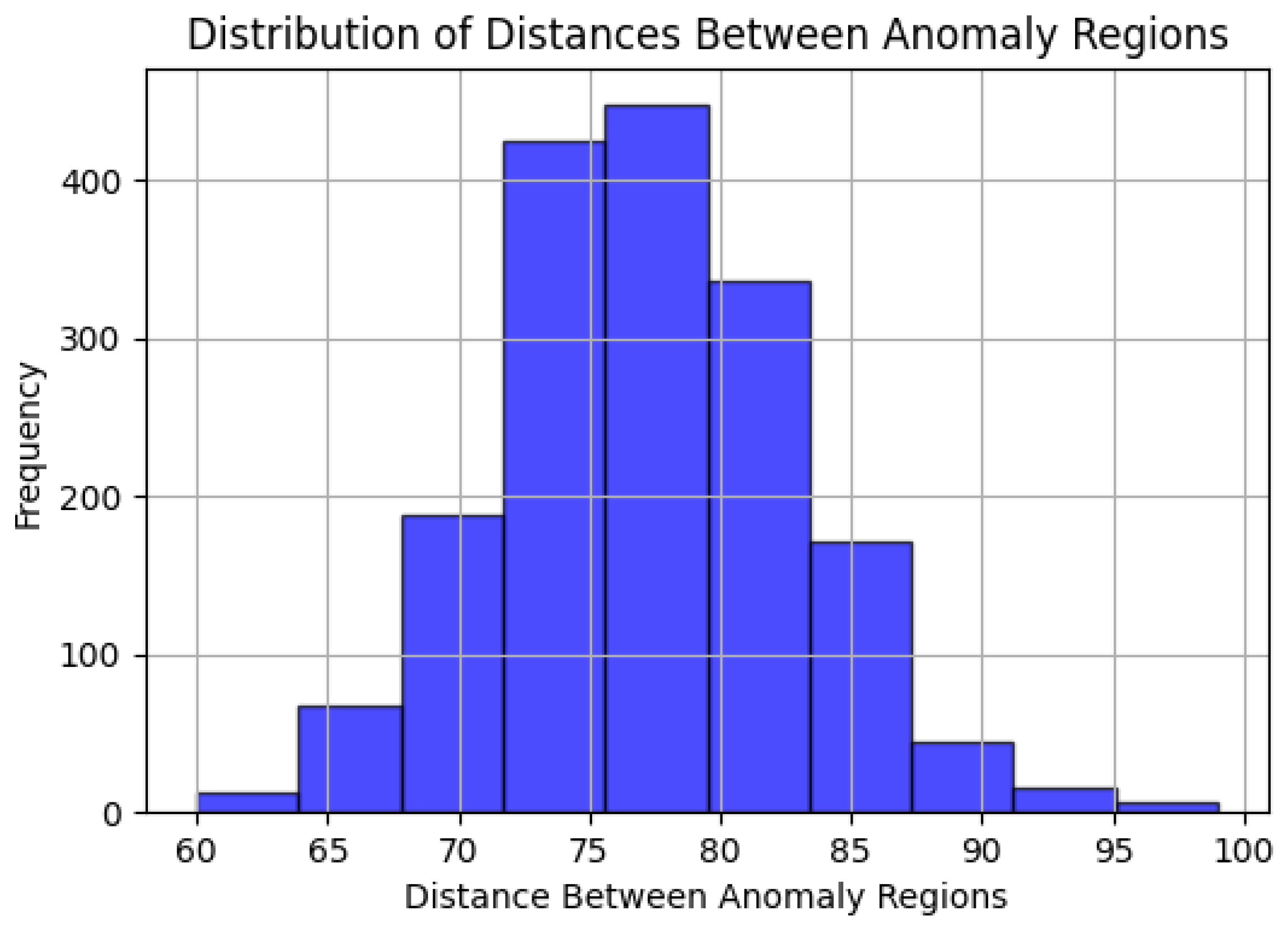Figure 4 presents a histogram of point distances between anomaly regions, while Figure 5 visualizes how many anomalies exist in each anomaly region. Our proposed model was tested and evaluated under conditions similar to the real-time anomaly detection challenges in industrial environments while considering the reduced anomaly rate and structured temporal patterns. In the diluted dataset, which was named WaterLog* dataset, the total number of samples is 132,319, consisting of 129,890 normal samples and 2429 attack samples. The dataset is divided into training and testing sets as follows: the training set includes 90,941 samples (1682 attack), while test set contains 39,696 samples (747 attack), ensuring a realistic evaluation scenario with a balanced representation of normal and anomalous instances.

Table 1. Data examples from the WaterLog* dataset.

DL	DP	TL	TF	TP	EL	EF	EP	CL	CPF	CVF	CP	CV	TKL	TVF	TV	Normal/Attack
30.0149228	1	13.8590722	1.24468854	1	11.6742456	2.29699343	1	9.71879086	2.39063017	2.32459778	1	1	12.2902877	2.83367948	1	0
25.83133	0	13.95848	3.179441	0	12.41807	0.361413	1	8.466223	4.634958	1.8914	1	1	11.87648	2.77475	1	1
24.6927828	1	8.96471562	1.78791916	1	16.7352582	2.73840959	1	13.947549	1.25502799	1.36270061	1	1	10.6815551	1.71719526	1	0
32.02082	1	12.71891	4.093682	0	12.29463	2.183986	1	10.49807	2.545136	2.595516	1	1	19.94649	0.070191	1	1

shows examples from WaterLog* dataset. A comparative summary table of all datasets mentioned in this section is presented in

Table 2. Comparison of anomaly detection datasets.

Dataset	Source	Data Type	Sensors Num.	Samples Num.	Application Area
MSL (Mars Science Laboratory)	Hundman et al. (2018) [28]	Time series (spacecraft telemetry)	27	∼73,000	Space exploration, fault detection
SMAP (Soil Moisture Active Passive)	Hundman et al. (2018) [28]	Time series (satellite telemetry)	55	∼56,000	Soil moisture measurement, remote sensing
SMD (Server Machine Dataset)	Su et al. (2019) [17]	Time series (server performance data)	38	28 million	Server failure detection, system monitoring
SWAT (Secure Water Treatment)	Mathur & Tippenhauer (2016) [29]	Sensor data (water treatment plant)	51	946,722	Industrial control system security
PSM (Pooled Server Metrics)	Abdulaal et al. (2021) [30]	Time series (IT infrastructure)	25	∼10 million	IT systems, network security
Pulp & Paper Dataset	Ranjan et al. (2018) [31]	Sensor data (paper manufacturing plant)	50+	Not specified	Industrial process analysis
WaterLog	Balta et al. (2025) [32]	Time Series (Potable water process)	16	180,000	Industrial control system security
WaterLog* (Diluted version of WaterLog)	Balta et al. (2025) [32]	Time Series (Potable water process)	16	∼132,000	Industrial control system security

.

5. Experimental Results and Performance Evaluation

To rigorously evaluate the proposed method, we conduct extensive experiments against five recent and widely adopted benchmark models in the field of time-series anomaly detection:

• LMSAutoTSF [20]: A learnable multi-scale architecture based on trend–seasonal decomposition.
• iTransformer [21]: Inverted transformer architecture separating variable and temporal tokens.
• TimeMixer [22]: A decomposable multi-scale mixing architecture.
• PatchTST [23]: A transformer variant optimized for long-term forecasting with patch-based input encoding.
• AnomalyTransformer [5]: A transformer-based model leveraging self-attention and an association discrepancy criterion for anomaly scoring.

All baseline models were retrained on the same datasets using their officially released code and configuration guidelines. The comparison metrics used are the following:

• F1-Score: The traditional harmonic mean of precision and recall in pointwise anomaly detection.
• (${F1}_{PA}$) (Point-Adjusted F1): A metric that considers a detection correct if it overlaps with a true anomaly window.
• (${F1}_{CPA}$) (Coverage-based F1): A stricter metric that requires a certain level of overlap (coverage) with the ground-truth anomaly duration.

In addition, we apply our sliding window dynamic thresholding technique not only to ChaMTeC but also to the baseline models. This ensures that the performance gains are due to architectural innovation and not simply better thresholding.

5.1. Model Configuration

The model operates on multivariate time series with F input features and reconstructs input sequences of length 100. A summary of the most relevant hyperparameter settings is shown in

Table 3. Hyperparameter settings of ChaMTeC for the WaterLog* dataset. For other datasets, the settings remain the same, except for the input feature dimension, which varies accordingly.

Hyperparameter	Value
Batch Size	128
Input Sequence Length	100
Input Features	16
Embedding Dimension	32
Number of Encoders	3
RNN Hidden Size	8
RNN Layers	8

.

5.2. Evaluation Metrics for Time-Series Anomaly Detection

In the context of time-series data, the direct application of the standard F1-score is challenging due to the inherent dissociation between time points and time events. To address this, anomaly predictions are typically adjusted using heuristic-based methods, commonly referred to as point adjustment (PA), prior to F1-score evaluation ($F_{1PA}$). However, these adjustments are often biased toward true positive detection, leading to an overestimation of detector performance. This limitation underscores the need for a more rigorous evaluation framework that better aligns with the temporal nature of anomalies and provides a fairer assessment of detection capabilities. To ensure a rigorous evaluation of time-series anomaly detection, we use a coverage-based point adjustment technique ($F_{1CPA}$), ensuring that predicted anomalies are validated by requiring a minimum overlap ratio with ground-truth anomaly segments. Only predictions with sufficient coverage are deemed correct, ensuring a more rigorous evaluation process.

5.3. Standard F1-Score (F1)

The F1-score is the harmonic mean of Precision and Recall, measuring the balance between false positives and false negatives.

$$F1=2\times {\displaystyle \frac{\mathrm{Precision}\times \mathrm{Recall}}{\mathrm{Precision}+\mathrm{Recall}}}$$

(20)

where

$$\mathrm{Precision}={\displaystyle \frac{TP}{TP+FP}}$$

(21)

$$\mathrm{Recall}={\displaystyle \frac{TP}{TP+FN}}$$

(22)

Here, $TP$ (True Positive) represents the correctly detected anomalies, $FP$ (False Positive) denotes normal points incorrectly identified as anomalies, and $FN$ (False Negative) corresponds to undetected anomalies.

The sequential and temporal nature of anomalies makes it difficult to apply the standard F1-score to time-series anomaly detection, even though it works well for discrete classification problems. Direct comparison between predicted and ground-truth anomalies may lead to unfair penalization or overestimation because anomalies happen over a range of time steps rather than isolated points.

5.4. Point-Adjusted F1-Score (F1_PA)

A predicted anomaly is deemed a true positive if it falls within any ground-truth anomaly segment according to the Point-Adjusted F1-Score (F1_PA), which introduces a heuristic modification to address the drawbacks of the standard F1-score in time-series settings. The following definitions of true positives, false positives, and false negatives are altered in this method:

• $T{P}_{PA}$ (Point-Adjusted True Positive): A predicted anomaly point is counted as a true positive if it overlaps with any ground-truth anomaly segment.
• $F{P}_{PA}$ (Point-Adjusted False Positive): A predicted anomaly that does not correspond to any ground-truth anomaly.
• $F{N}_{PA}$ (Point-Adjusted False Negative): A ground-truth anomaly with no overlapping predicted anomaly points.

Using these adjusted values, the point-adjusted F1-score is calculated as follows:

$$F{1}_{PA}=2\times {\displaystyle \frac{{\mathrm{Precision}}_{PA}\times {\mathrm{Recall}}_{PA}}{{\mathrm{Precision}}_{PA}+{\mathrm{Recall}}_{PA}}}$$

(23)

where

$${\mathrm{Precision}}_{PA}={\displaystyle \frac{T{P}_{PA}}{T{P}_{PA}+F{P}_{PA}}}$$

(24)

$${\mathrm{Recall}}_{PA}={\displaystyle \frac{T{P}_{PA}}{T{P}_{PA}+F{N}_{PA}}}$$

(25)

By taking time-continuous anomalies into account, ${F1}_{PA}$ enhances the standard F1-score; however, it introduces a bias towards true positive detection, which may lead to an overestimation of model performance. This problem occurs because, even in cases where the model is unable to identify the majority of the anomaly duration, a single correctly detected anomaly point within an interval is enough to count the entire interval as correctly detected.

5.5. Coverage-Based Point-Adjusted F1-Score (F1_CPA)

We use the Coverage-Based Point-Adjusted F1-Score (F1_CPA) to get around the drawbacks of ${F1}_{PA}$. This method refines true positive evaluation by requiring a minimum overlap ratio between predicted and actual anomaly segments. A predicted anomaly is only regarded as a true positive in this method if it satisfies a predetermined coverage threshold.

$${\mathrm{Precision}}_{CPA}={\displaystyle \frac{{\sum }_i|A_i\cap P_i|}{{\sum }_i\left|P_i\right|}}$$

(26)

$${\mathrm{Recall}}_{CPA}={\displaystyle \frac{{\sum }_i|A_i\cap P_i|}{{\sum }_i\left|A_i\right|}}$$

(27)

where

• $A_i$ represents the ground-truth anomaly segments.
• $P_i$ denotes the predicted anomaly segments.
• $|A_i\cap P_i|$ is the length of the intersection between the predicted and ground-truth anomaly segments.
• $|P_i|$ is the total predicted anomaly duration.
• $|A_i|$ is the total ground-truth anomaly duration.

Using these coverage-based definitions, the final ${F1}_{CPA}$ score is computed as follows:

$$F{1}_{CPA}=2\times {\displaystyle \frac{{\mathrm{Precision}}_{CPA}\times {\mathrm{Recall}}_{CPA}}{{\mathrm{Precision}}_{CPA}+{\mathrm{Recall}}_{CPA}}}$$

(28)

By penalizing predictions that do not adequately cover the actual anomaly period, this metric guarantees a more realistic evaluation. ${F1}_{CPA}$ offers a more stringent evaluation of the model’s capacity to capture anomalies as continuous events, in contrast to F1_PA, which has the potential to distort performance by favoring scattered detections.

Our dataset, WaterLog*, is particularly well suited for evaluating anomaly detection methods due to its unique characteristics. Unlike many public benchmarks that contain frequent and densely packed anomalies, WaterLog* features sparse and isolated anomaly regions. This sparsity mirrors real-world scenarios where anomalies are rare and often localized, making it a more challenging and realistic candidate for evaluation. By leveraging this dataset, we can better distinguish between methods that perform well in detecting sparse anomalies and those that rely on frequent anomaly occurrences.

Table 4. Comparison of the evaluation metrics on the WaterLog* dataset.

Thresh	Metric	ChaMTeC (Ours) w/o Attention	ChaMTeC (Ours)	LMS AutoTSF	iTransformer	TimeMixer	PatchTST	Anomaly Trans
Fixed	$F_1$	0.1942	0.3674	0.1844	0.1785	0.2593	0.2228	0.2617
	$F_{1PA}$	0.2725	0.3804	0.2308	0.2599	0.2803	0.2695	0.2894
	$F_{1CPA}$	0.2725	0.3804	0.2308	0.2599	0.2803	0.2695	0.2894
Sliding window	$F_1$	0.2635	0.3246	0.1287	0.2210	0.2190	0.1632	0.5125
	$F_{1PA}$	0.3861	0.4635	0.1915	0.3284	0.3309	0.2405	0.5959
	$F_{1CPA}$	0.3861	0.4635	0.1915	0.3284	0.3309	0.2405	0.5959

demonstrates that $F_1$ and $F_{1CPA}$ give the same results because WaterLog* does not contain large anomaly regions; on the other hand, adjustments in the other datasets have a huge effect on the results, as seen in

Table 5. Comparison of the evaluation metrics on the MSL dataset.

Thresh	Metric	ChaMTeC (Ours) w/o Attention	ChaMTeC (Ours)	LMS AutoTSF	iTransformer	TimeMixer	PatchTST	Anomaly Trans
Fixed	$F_1$	0.0529	0.0528	0.0673	0.0601	0.0630	0.0664	0.0649
	$F_{1PA}$	0.8017	0.7638	0.7423	0.7987	0.7945	0.7926	0.8184
	$F_{1CPA}$	0.1590	0.1460	0.1634	0.1363	0.1446	0.1484	0.1340
Sliding window	$F_1$	0.0503	0.0486	0.0614	0.0473	0.0521	0.0473	0.0440
	$F_{1PA}$	0.8289	0.8299	0.8079	0.8248	0.8449	0.8370	0.8249
	$F_{1CPA}$	0.1852	0.1614	0.2186	0.1588	0.1749	0.1472	0.1449

. To evaluate the effectiveness of our proposed anomaly detection approach, we conduct an ablation study on two benchmark datasets: the MSL dataset and WaterLog dataset. We compare the performance of five state-of-the-art methods—LMSAutoTSF [20], iTransformer [21], TimeMixer [22], PatchTST [23], and AnomalyTransformer [5]—under two thresholding approaches: Fixed Thresholding and Sliding Window Thresholding (thFactor = 2.0). For a comprehensive evaluation, we utilize three metrics: $F_1$, $F_{1PA}$, and $F_{1CPA}$. Additionally, we evaluate two variants of our proposed architecture with and without an attention (w/o) mechanism to analyze the impact of attention components, as detailed in all tables containing results.

5.6. Thresholding Approaches and Metrics

Fixed Thresholding: This approach uses a static threshold value for detecting anomalies. While it is straightforward to implement, it lacks the adaptability required for datasets where anomaly magnitudes vary over time.

Sliding Window Thresholding: This dynamic approach computes the threshold as a moving average with a deviation factor. It adapts to variations in anomaly magnitude and enhances the detection of extended anomaly regions.

${\mathit{F}}_{\mathbf{1}\mathbf{CPA}}$: In addition to the traditional $F_1$ score and pointwise precision-adjusted score ($F_{1PA}$), we adopt $F_{1CPA}$ (Coverage-based Precision-Adjusted $F_1$) for evaluation. This metric accounts for the temporal continuity of anomalies, rewarding models that detect anomalies consistently across their entire duration. Unlike $F_1$, which measures pointwise accuracy, $F_{1CPA}$ ensures that anomalies are treated as coherent regions, making it more suited for real-world applications where anomalies often span multiple time steps.

5.7. Performance Comparison

Table 6. Anomaly detection performance on the WaterLog* dataset (threshold with sliding window: thFactor = 2.0). The values highlighted in red and blue indicate the best and second best scores for each metric.

Metric	ChaMTeC (Ours) w/o Attention	ChaMTeC (Ours)	LMS AutoTSF	iTransformer	TimeMixer	PatchTST	Anomaly Trans
$P_{CPA}$	0.3534	0.4312	0.1417	0.2785	0.2632	0.1743	0.4797
$R_{CPA}$	0.4253	0.5011	0.2954	0.4000	0.4452	0.3880	0.7866
$F_{1CPA}$	0.3861	0.4635	0.1915	0.3284	0.3309	0.2405	0.5959

and

Table 7. Anomaly detection performance (threshold with sliding window: thFactor = 2.0). The values highlighted in red and blue indicate the best and second best average scores for each metric.

Dataset	Metric	ChaMTeC (Ours) w/o Attention	ChaMTeC (Ours)	LMS AutoTSF	iTransformer	TimeMixer	PatchTST	Anomaly Trans
MSL	$P_{CPA}$	0.3225	0.2901	0.3100	0.2725	0.3168	0.2761	0.2587
	$R_{CPA}$	0.1299	0.1118	0.1688	0.1120	0.1208	0.1004	0.1006
	$F_{1CPA}$	0.1852	0.1614	0.2186	0.1588	0.1749	0.1472	0.1449
PSM	$P_{CPA}$	0.5186	0.5245	0.4320	0.4942	0.5484	0.4681	0.5089
	$R_{CPA}$	0.1018	0.1084	0.0824	0.0913	0.1333	0.0907	0.0876
	$F_{1CPA}$	0.1702	0.1797	0.1384	0.1541	0.2145	0.1520	0.1495
SMAP	$P_{CPA}$	0.4369	0.5497	0.5034	0.3567	0.4283	0.4899	0.6634
	$R_{CPA}$	0.6392	0.5424	0.2254	0.2845	0.3892	0.3440	0.5294
	$F_{1CPA}$	0.5190	0.5460	0.3113	0.3165	0.4078	0.4042	0.5889
SMD	$P_{CPA}$	0.3341	0.3237	0.3043	0.3156	0.3287	0.3313	0.2959
	$R_{CPA}$	0.5842	0.5603	0.4688	0.5327	0.5382	0.5352	0.5595
	$F_{1CPA}$	0.4251	0.4103	0.3691	0.3963	0.4081	0.4092	0.3871
SWAT	$P_{CPA}$	0.6897	0.3629	0.1615	0.6926	0.6957	0.1951	0.2155
	$R_{CPA}$	0.7685	0.2061	0.0572	0.7462	0.8129	0.0758	0.0656
	$F_{1CPA}$	0.7270	0.2629	0.0845	0.7184	0.7497	0.1092	0.1006
Average	$P_{CPA}$	0.4604	0.4102	0.3422	0.4263	0.4636	0.3521	0.3885
	$R_{CPA}$	0.4447	0.3058	0.2005	0.3533	0.3989	0.2292	0.2685
	$F_{1CPA}$	0.4053	0.3121	0.2244	0.3488	0.3910	0.2444	0.2742

present comprehensive experimental results comparing ChaMTeC with state-of-the-art models across multiple benchmark datasets. The evaluation metrics include the Point-wise Precision ($P_{CPA}$), Recall ($R_{CPA}$), and F1-score ($F_{1CPA}$), which are widely used in anomaly detection tasks. Our proposed ChaMTeC model demonstrates superior overall performance, achieving the highest average F1-CPA score of 0.4053 without attention and 0.3121 with attention across all public benchmark datasets. This significantly outperforms recent state-of-the-art approaches, namely, LMSAutoTSF (0.2244), iTransformer (0.3488), TimeMixer (0.3910), PatchTST (0.2444), and AnomalyTransformer (0.2742). The performance advantage is particularly evident in the precision and recall metrics, where ChaMTeC achieves balanced scores of $P_{CPA}=0.4604$ and $R_{CPA}=0.4447$, indicating its robust detection capability without sacrificing accuracy.

On individual datasets, ChaMTeC shows exceptional performance on the SWAT dataset, achieving an F1-CPA score of 0.7270 and 0.2629 without and with attention, respectively. This is comparable to TimeMixer (0.7497), and it substantially outperforms LMSAutoTSF (0.0845), PatchTST (0.1092), and AnomalyTransformer (0.1006). The strong performance on SWAT, a complex industrial control system dataset, demonstrates our model’s effectiveness in real-world scenarios. Similarly, on our newly introduced WaterLog dataset, ChaMTeC achieves an F1-CPA of 0.3861 and 0.4635, consistently outperforming most baseline models (LMSAutoTSF: 0.1915, iTransformer: 0.3284, TimeMixer: 0.3309, PatchTST: 0.2405). Our experimental results demonstrate that while AnomalyTransformer achieves superior performance on the Waterlog dataset when combined with our proposed dynamic thresholding approach (as detailed in Table 4), our method consistently outperforms all baseline approaches across the majority of the evaluated datasets. This comprehensive evaluation highlights the robustness and generalizability of our proposed framework. On the other hand, the analysis reveals an important nuance: while temporal attention mechanisms significantly improve detection accuracy for the Waterlog dataset, they prove less effective for the other datasets. This dataset-dependent performance variation suggests that our temporal attention mechanisms require more sophisticated anomaly-specific adaptations, particularly in handling diverse anomaly duration scales, varying temporal dependencies across different sensor types, and complex multi-variate interaction patterns.

These comprehensive results validate that our proposed architecture’s key components—inverted embedding, temporal encoding, and the MSE-based feedback mechanism with dynamic thresholding—work synergistically to enhance anomaly detection performance across diverse datasets. The consistent superior performance, particularly on industrial datasets such as SWAT and WaterLog, demonstrates ChaMTeC’s practical utility in real-world applications.

6. Conclusions

In this paper, we presented ChaMTeC, a novel time-series anomaly detection framework that combines inverted embedding, temporal encoding, and MSE-based feedback mechanisms with dynamic thresholding. Our experimental results demonstrate that ChaMTeC outperforms most of the existing state-of-the-art models across multiple benchmark datasets. In addition, when an ablation study was conducted to evaluate the contribution of each component of the ChaMTeC model to the performance, it was observed that the Inverted embedding component strengthened the model’s ability to detect subtle anomalies in time-series data, and when it was removed, there was a significant decrease in the F1-CPA score. Temporal encoding plays a critical role in understanding time-dependent anomalies, and when it was removed, there was a decrease in the recall rate. Finally, the MSE-based feedback loop and dynamic thresholding increase the accuracy by continuously adjusting the model’s detection thresholds; when this component was removed, there was a significant decrease in precision. These results reveal how each component contributes to the overall performance of ChaMTeC and the model’s anomaly detection ability.

The framework’s effectiveness is particularly evident in its robust performance on complex industrial datasets such as SWAT and our newly introduced WaterLog dataset. Our results suggest that the combination of channel-mixing techniques and temporal convolutional networks, along with our dynamic thresholding approach, is particularly effective for detecting subtle anomalies in industrial control systems. Future work could explore the adaptation of our framework to other domains and the integration of additional context-aware features to further improve detection accuracy. However, we observe that the inclusion of attention mechanisms in our architecture introduces dataset-dependent performance variations. This suggests that standard attention mechanisms may not sufficiently capture anomaly-specific temporal patterns in certain contexts. While ChaMTeC demonstrates strong anomaly detection performance, certain types of anomalies remain challenging, particularly long-duration anomalies, abrupt pattern shifts, and cross-sensor dependencies. Long-duration anomalies spanning multiple sliding windows are harder to detect due to the model’s focus on recent temporal patterns, while abrupt shifts in volatile signals can be mistaken for transient fluctuations. Additionally, complex dependencies between multiple sensor readings in datasets such as WaterLog pose difficulties, as standard feature extraction methods may overlook subtle correlations. Interestingly, while attention mechanisms enhance performance on WaterLog by capturing long-range dependencies, they prove less effective for datasets such as SWAT, where anomalies are more localized. This suggests that standard attention mechanisms may not always align with diverse anomaly types. Future improvements could incorporate sparse attention, dynamic feature gating, and hierarchical temporal modeling to enhance adaptability, ensuring robust detection across various real-world industrial settings.

A significant contribution of this work is the introduction of the WaterLog dataset, which we have made publicly available to the research community. Unlike existing datasets, WaterLog was specifically restructured to reflect real-world industrial control system environments, where anomalies are rare events. By reducing the anomaly rate and restructuring the data distribution, we provide a more realistic benchmark for evaluating anomaly detection systems in industrial settings. This addresses a critical gap in existing benchmarks, which often fail to capture the true challenges of real-time anomaly detection in operational environments.