
Comparative Evaluation of Feed-Forward Neural Networks for Predicting Uniaxial Compressive Strength of Seybaplaya Carbonate Rock Cores


Abstract

1. Introduction
- Direct Algorithmic Comparison. We implement and rigorously compare four feed-forward ANN architectures (RBF, BR, SCG, LM) on a uniform dataset of 50 Seybaplaya carbonate core specimens, leveraging identical preprocessing pipelines, data split protocols, and performance metrics.
- Statistical Validation. Through 30 independent training–testing runs per model and hypothesis testing via the Friedman test with Benjamini–Hochberg correction, we objectively determine the statistical significance of inter-algorithm performance differences.
- Feature Importance Analysis. Employing a partial derivatives sensitivity analysis, we quantify the relative influence of water content, porosity, and density on UCS predictions, providing actionable insight into variable prioritization for field measurements.
- Practical Recommendations. We synthesize our findings into clear recommendations for selecting ANN training strategies that balance predictive accuracy, convergence efficiency, and generalization robustness in karst-affected carbonate engineering applications.
1.1. Comprehensive Multi-Algorithm Comparison
1.2. Statistically Validated Performance Ranking
1.3. Sensitivity-Driven Feature Importance Analysis
1.4. Guidelines for Model Selection in Karst-Influenced Carbonates
1.5. Data Resource for Seybaplaya Formation
2. Related Works
2.1. Empirical and Regression-Based Models
2.2. Water Content, Porosity, and Density Effects
2.3. Neural Network Applications in Geomechanics
2.4. Hybrid and Optimization Frameworks
2.5. Comparative Machine Learning and Regression Studies in Geomechanics
3. Materials and Methods
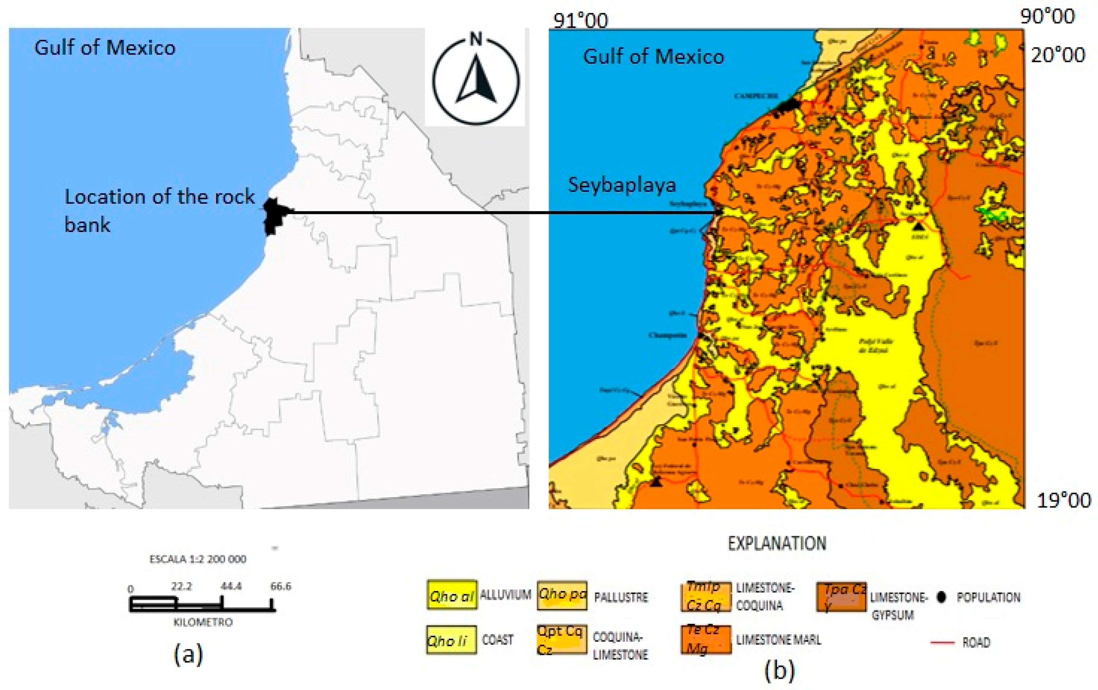
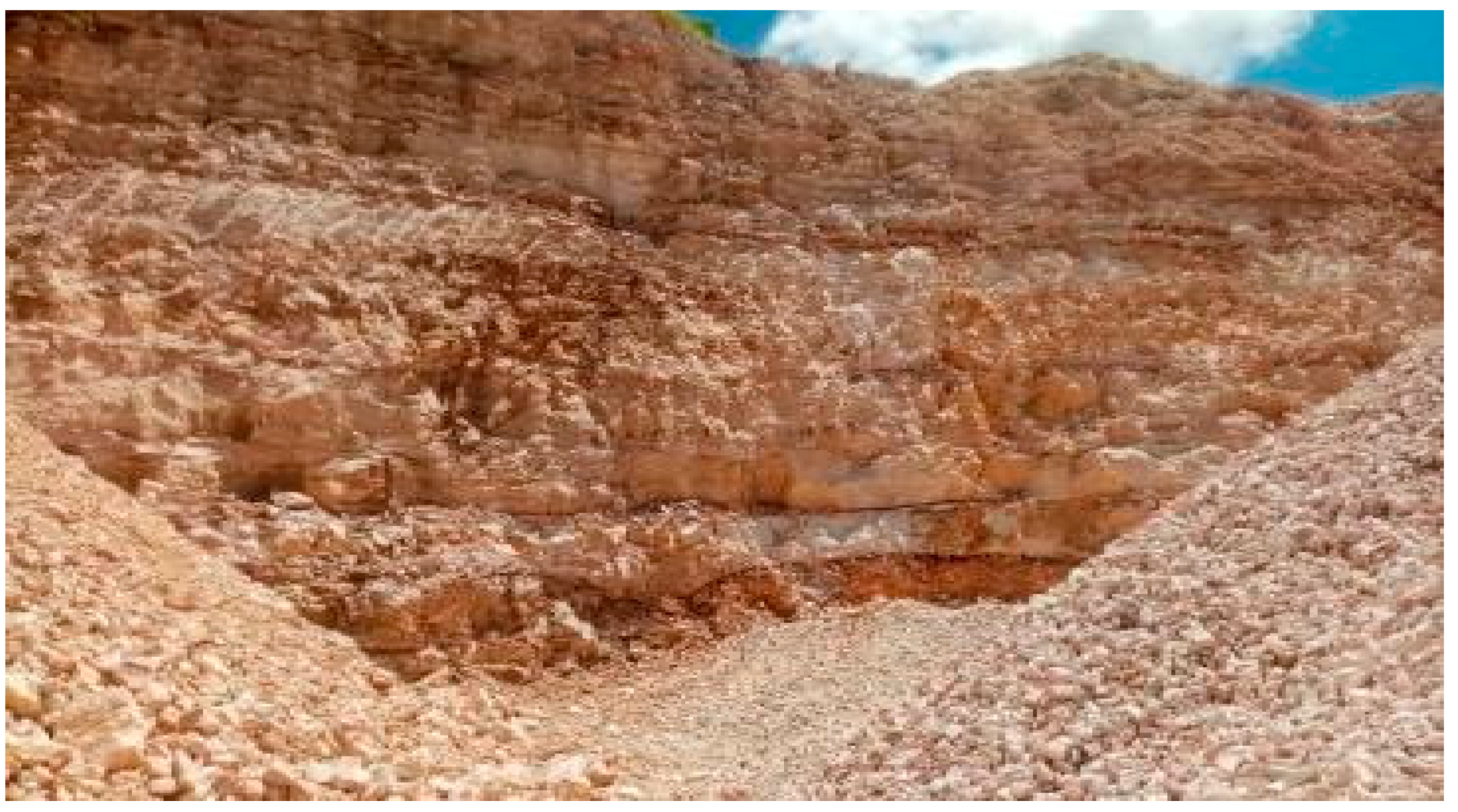
3.1. Study Site Location and Sampling
3.2. Rock Material Testing and Database
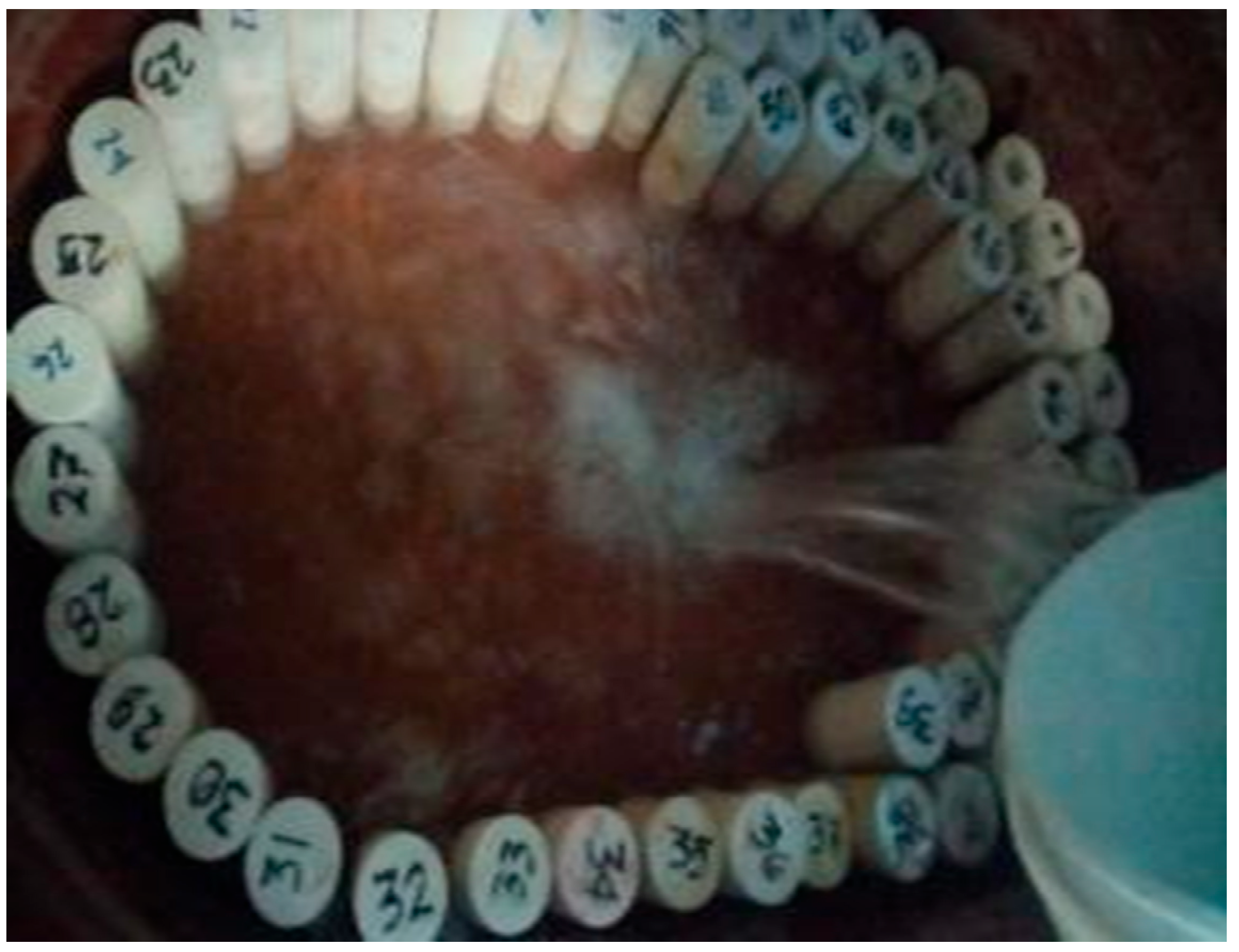
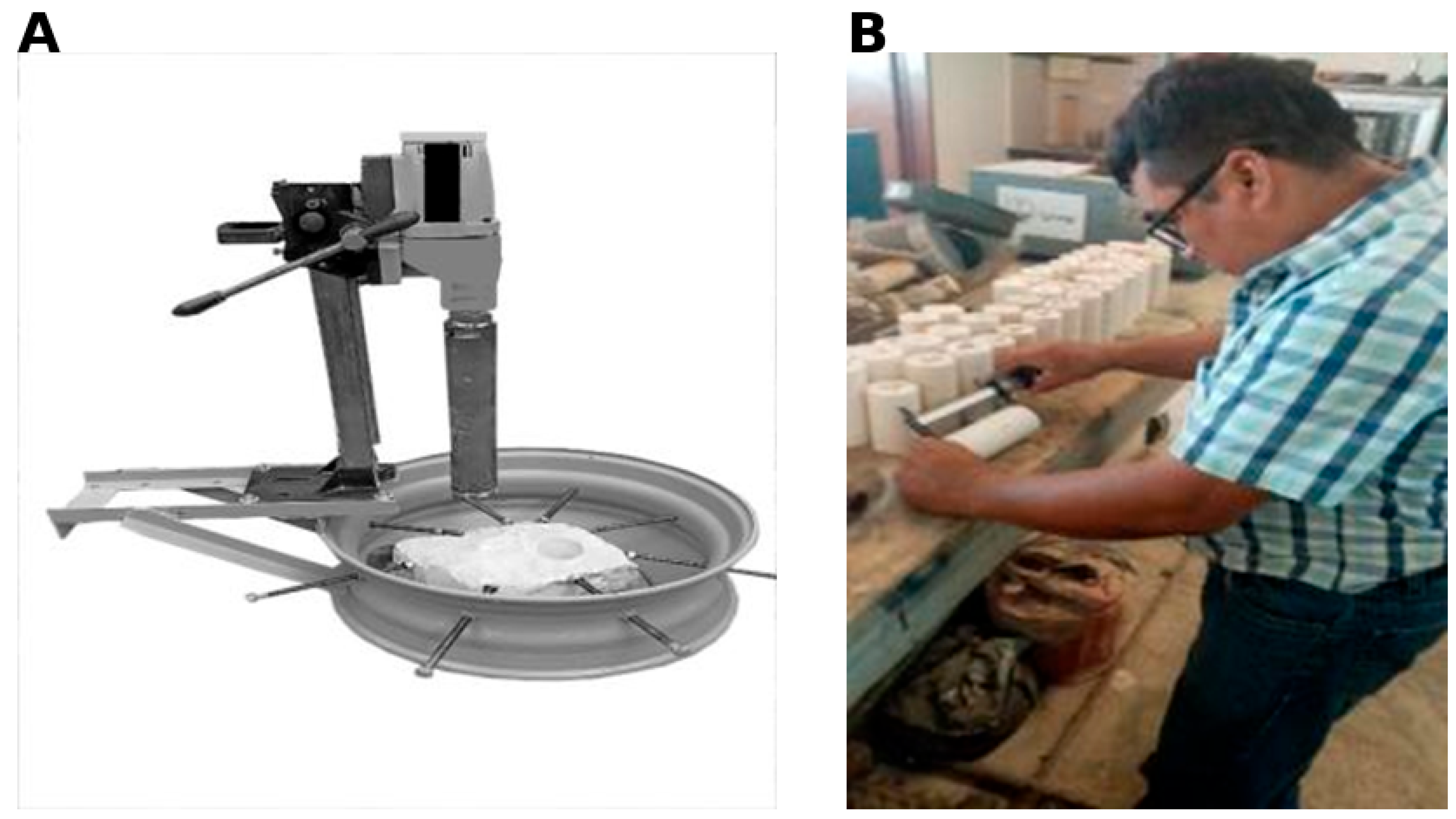
3.2.1. Quarry Exploration
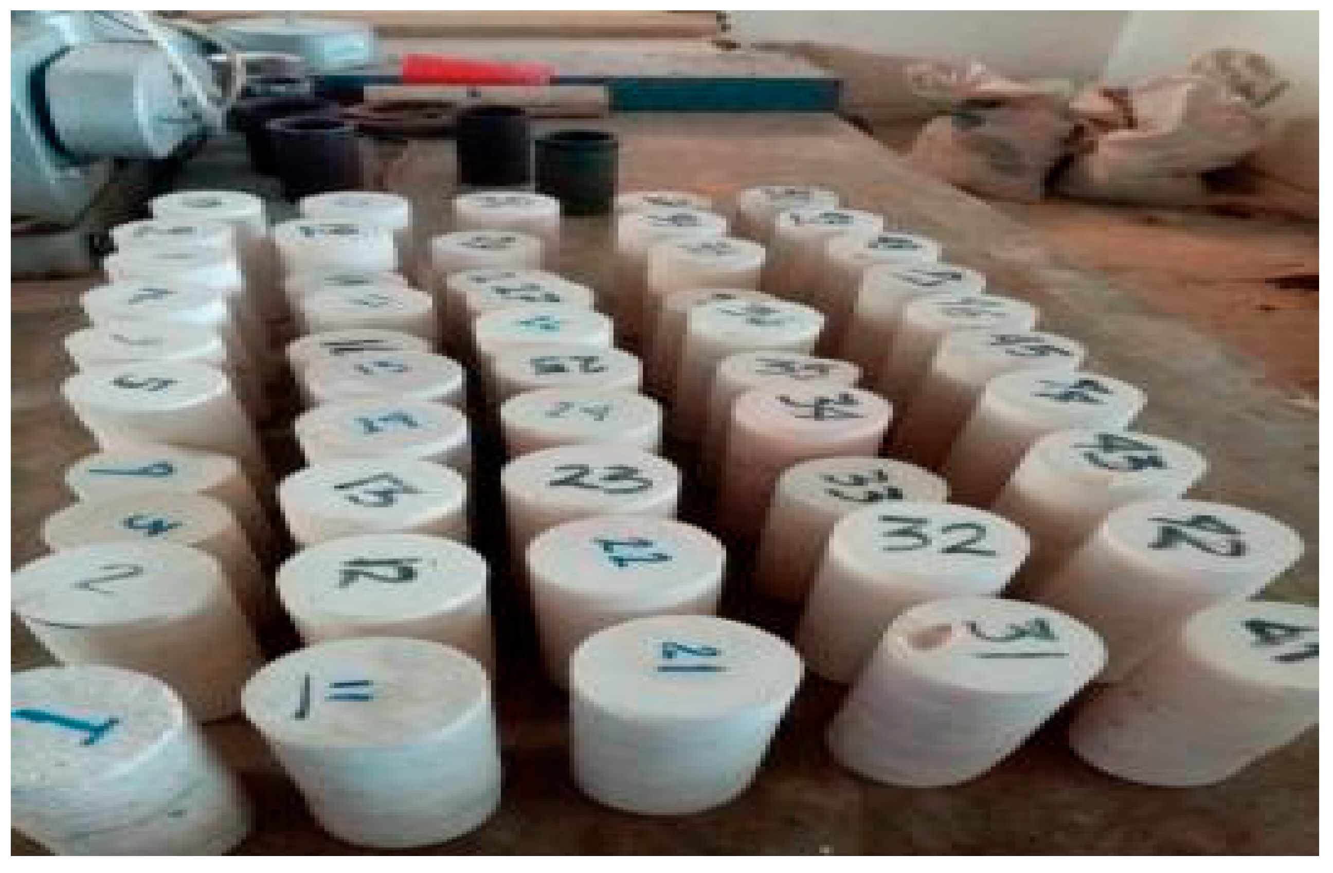
3.2.2. Sample Size
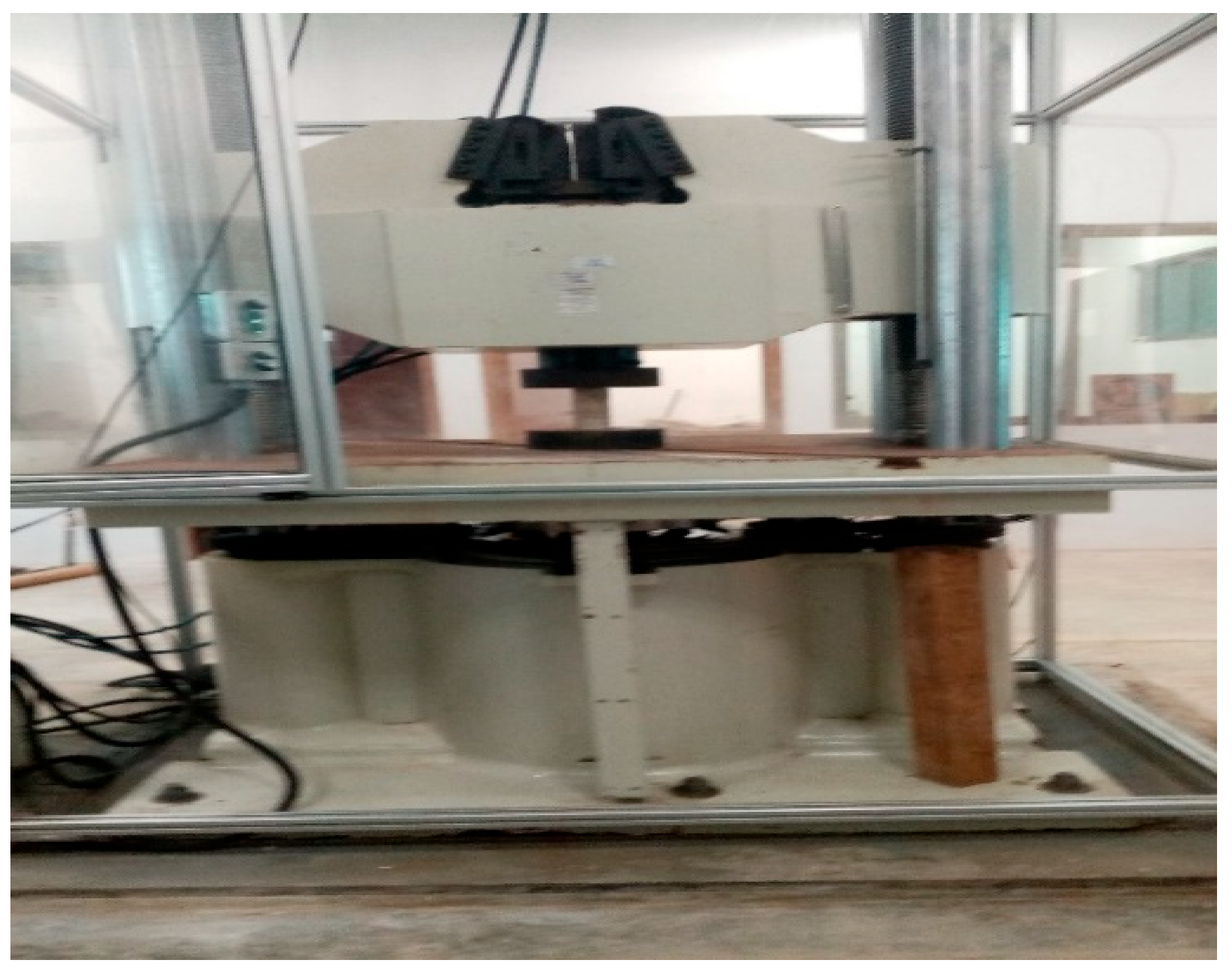
3.2.3. Laboratory Testing Methods
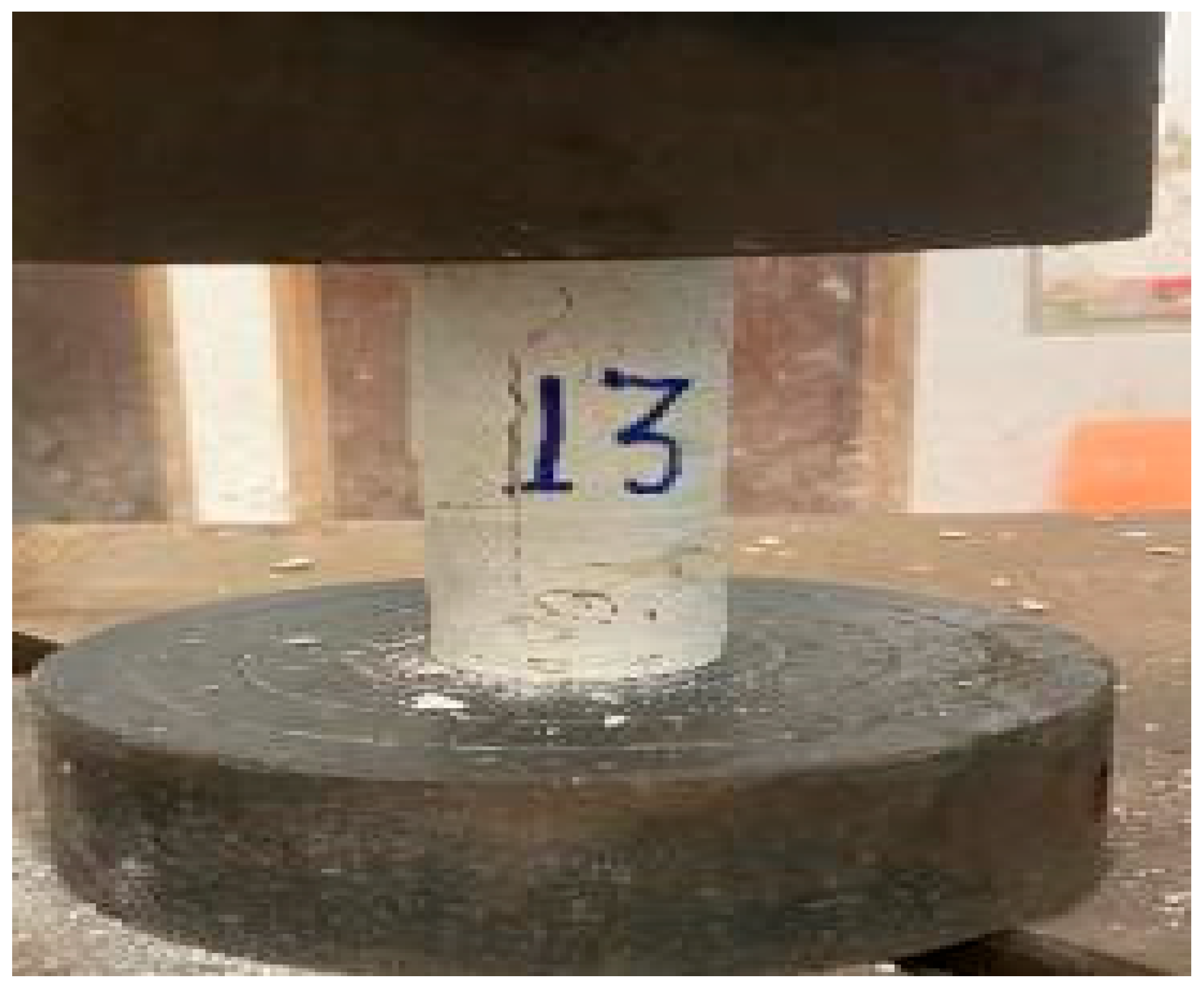
3.2.4. Uniaxial Compressive Strength (UCS)
3.2.5. Water Content
3.2.6. Real Density Test
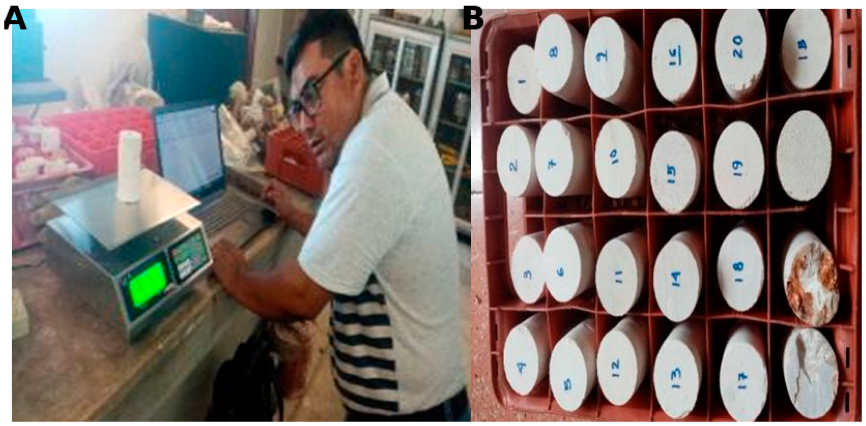
3.2.7. The Procedures for Determining the Rock’s True Density
3.2.8. Interconnected Porosity
3.2.9. Database
4. Neural Network Architectures for Uniaxial Compressive Strength Prediction
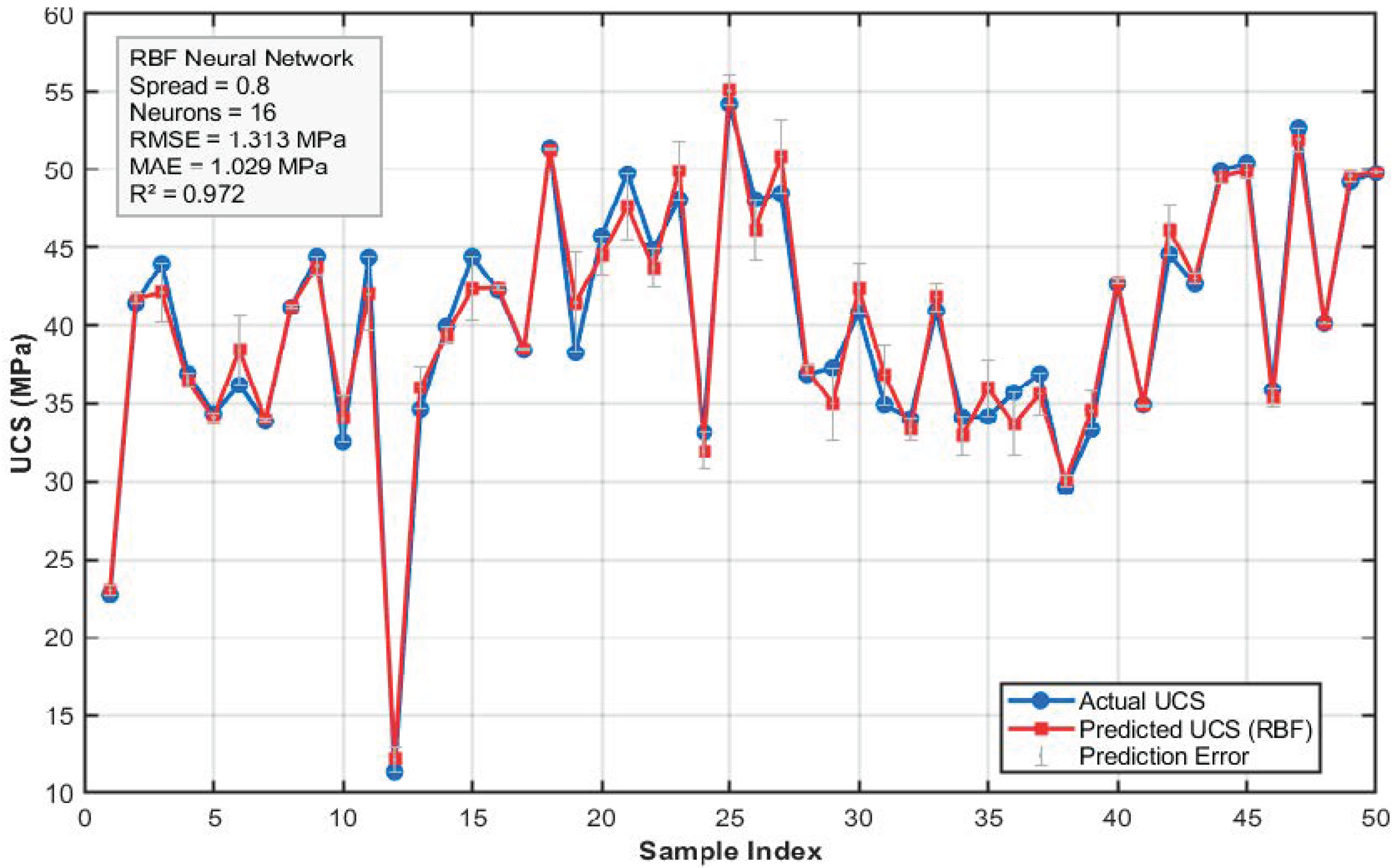
4.1. Radial Basis Function (RBF) Neural Network
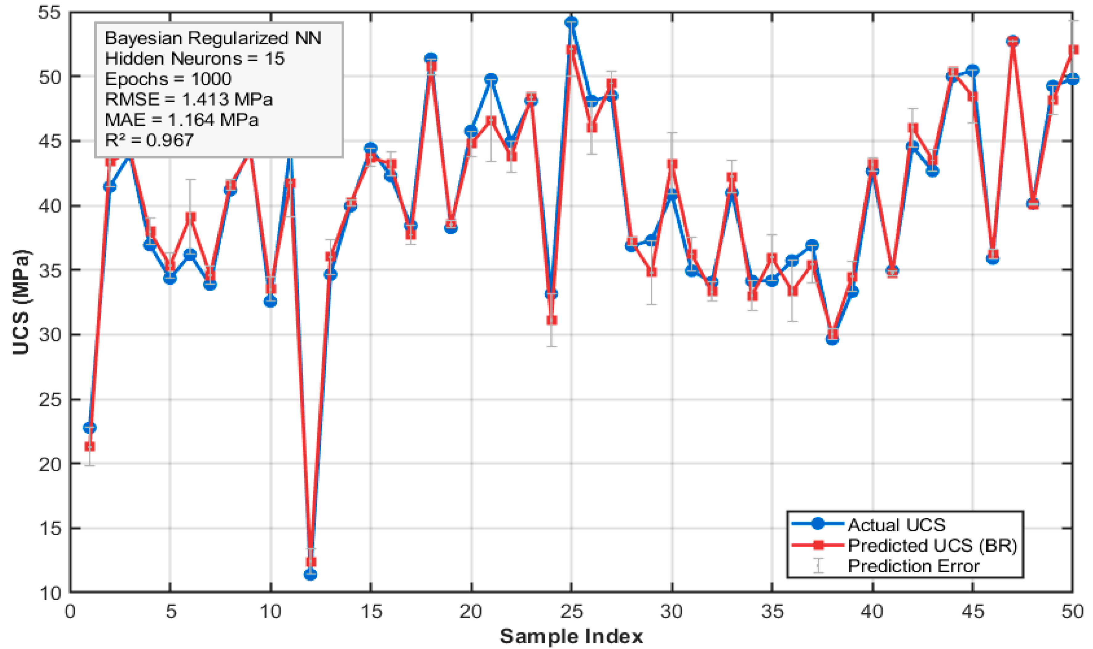
4.2. Bayesian Regularized Feed-Forward Neural Network
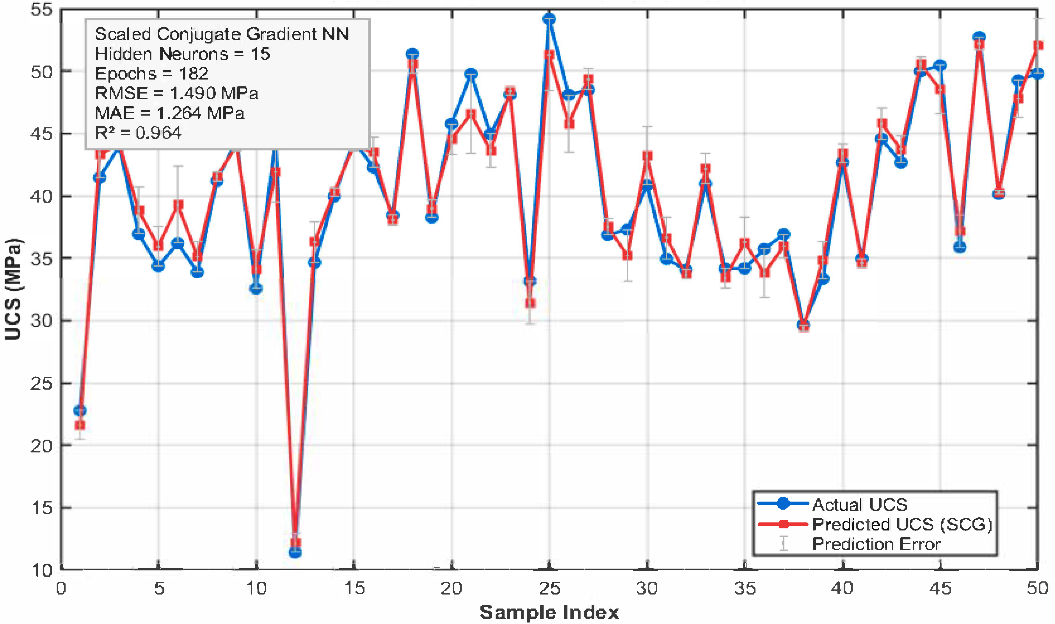
4.3. Scaled Conjugate Gradient (SCG) Neural Network
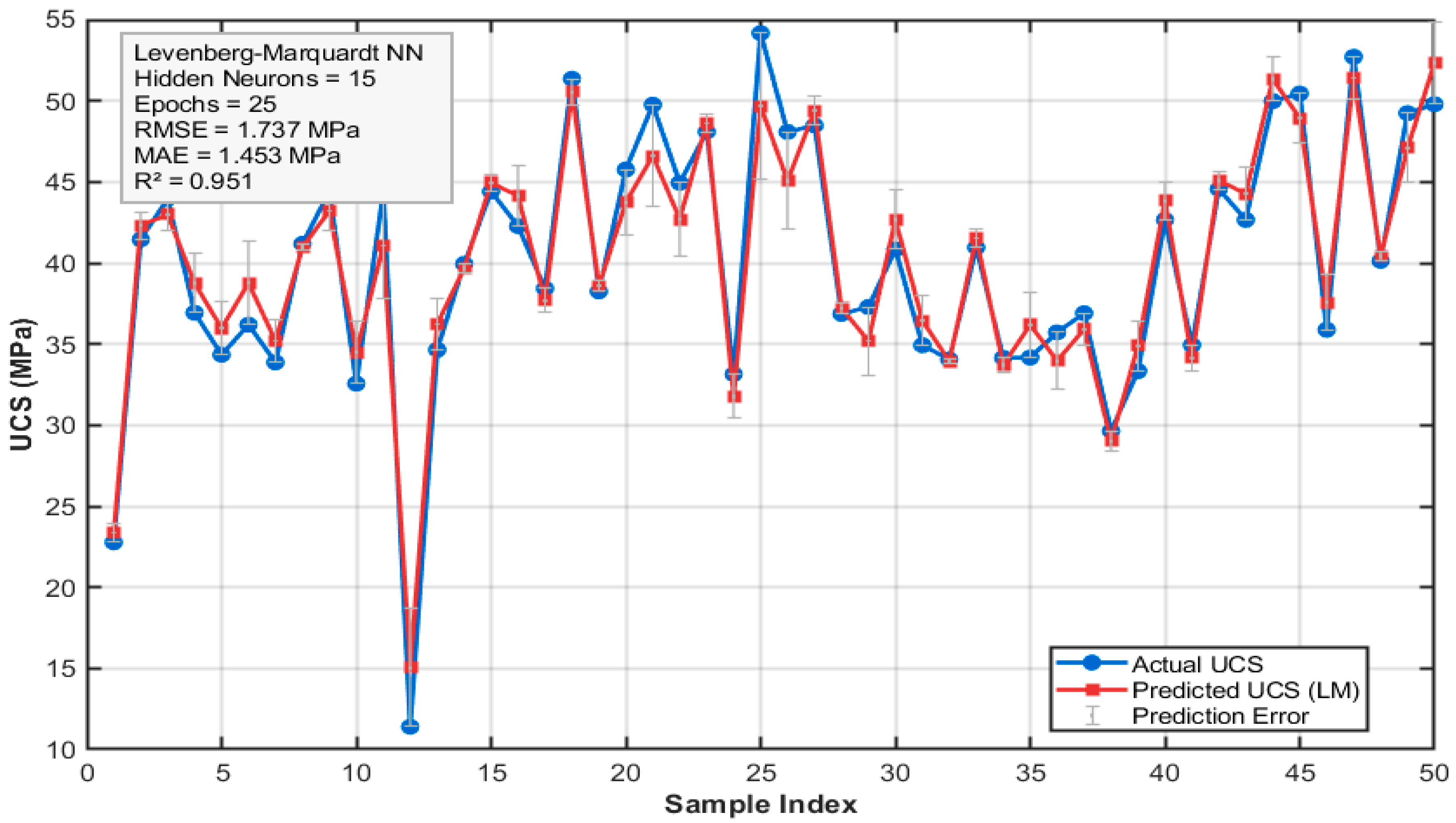
4.4. Levenberg–Marquardt (LM) Neural Network
5. Performance Evaluation Metrics
5.1. Mean Absolute Error (MAE)
5.2. Root Mean Square Error (RMSE)
5.3. Mean Absolute Percentage Error (MAPE)
5.4. Coefficient of Determination (COD)
6. Results and Discussion
6.1. Descriptive Statistics of the Experimental Dataset Variables
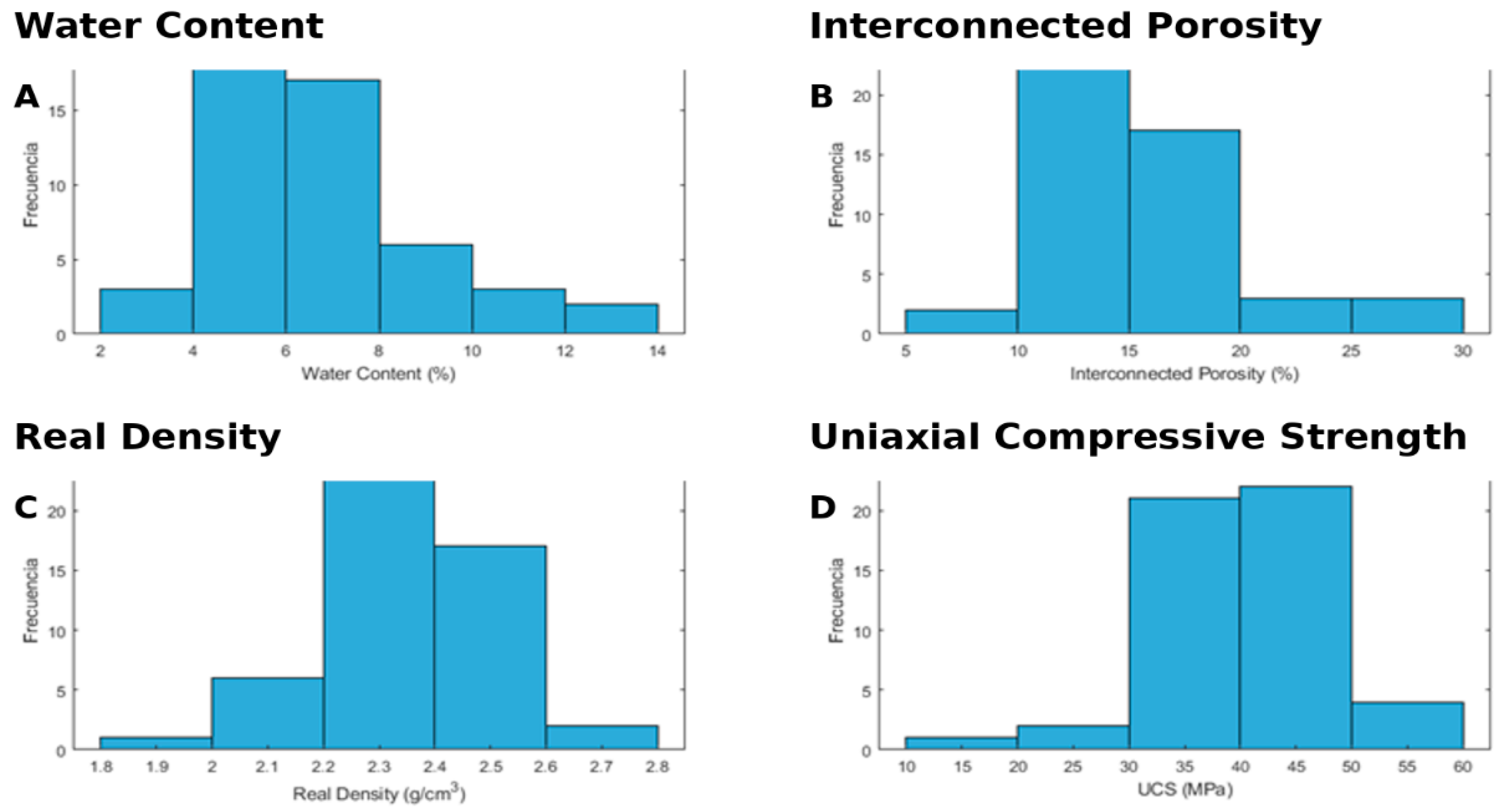
- Water Content (%): The moisture content exhibits an approximately bell-shaped distribution centered at 6–7%, with the majority (≈70%) falling between 4% and 9%. A slight rightward skew is apparent, as a small number of specimens reach up to 13–14%. This skew suggests occasional high-moisture outliers, which may influence rock weakening.
- Interconnected Porosity (%): Porosity values are concentrated between 10% and 20%, peaking around 12–15%. The distribution is mildly right-skewed, with a tail extending toward 28%, indicating that most rocks share similar characteristics, while a few exhibit significantly higher void space.
- Real Density (g/cm3): Density measurements cluster tightly between 2.2 and 2.5 g/cm3, with a modal of 2.3–2.4 g/cm3 and very few values below 2.1 g/cm3 or above 2.6 g/cm3. This narrow spread reflects a relatively homogeneous lithology across the rock bank.
- Uniaxial Compressive Strength (UCS, MPa): The strength distribution spans 11 MPa to 60 MPa, with about ≈75% between 30 MPa and 50 MPa. The histogram shows a mild right skew, driven by a few robust specimens. The central tendency around 35–45 MPa underscores the variability in mechanical resistance, which is essential for robust predictive modeling.
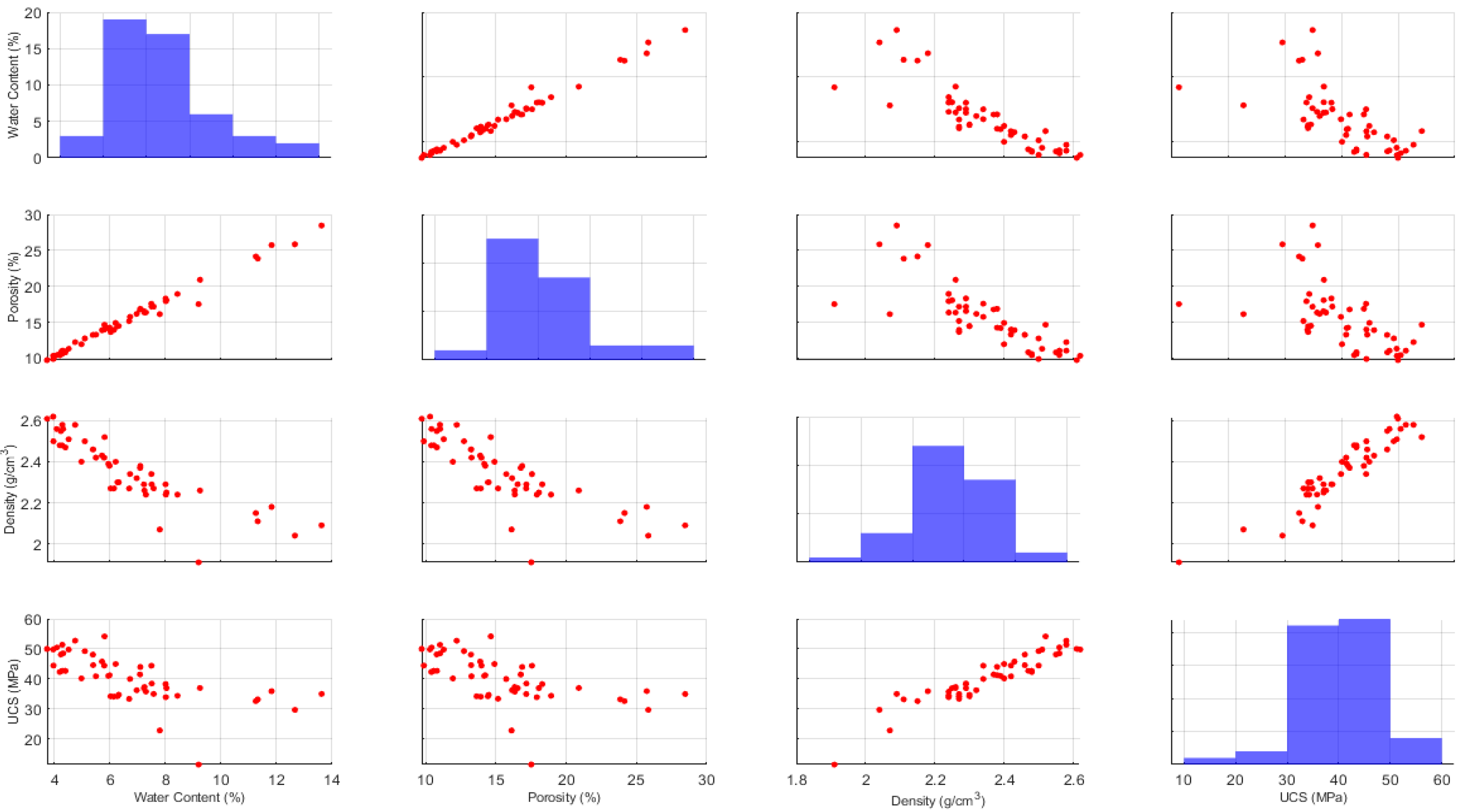
6.1.1. Diagonal Histograms
- Water content concentrates between 4% and 9%, confirming the moderate moisture range noted previously.
- Porosity predominantly ranges from 12% to 17%, with only a few samples exhibiting values above 25%.
- Density is tightly clustered near 2.3–2.5 g/cm3.
- UCS shows a dominant band from 30 MPa to 50 MPa, matching the earlier histogram.
6.1.2. Water Content vs. Porosity
- A strong positive linear (r ≈ 0.85) indicates that wetter specimens tend to exhibit higher porosity, likely reflecting pore filling by moisture (upper-left scatter).
6.1.3. Water Content vs. Density
- A moderate negative correlation (r ≈ –0.65) indicates that samples with higher moisture content generally exhibit lower dry density (lower-left cluster on the scatter plot), as expected when porosity increases
6.1.4. Water Content vs. UCS
- A weak to moderate negative correlation indicates that higher moisture content is generally associated with reduced mechanical strength. However, the considerable scatter suggests that additional factors also affect UCS.
6.1.5. Porosity vs. Density
- Porosity and density are inversely related (r ≈ –0.72), confirming that greater void space corresponds to lower bulk density (second-row, first-column scatter).
6.1.6. Porosity vs. UCS
- A negative correlation (r ≈ –0.78) indicates that samples with higher porosity exhibit lower UCS, underscoring porosity’s critical role in strength reduction.
6.1.7. Density vs. UCS
- A strong positive correlation (r ≈ 0.80) indicates that denser rocks resist compressive loading more effectively, making density one of the most predictive features for UCS (bottom-right scatter).
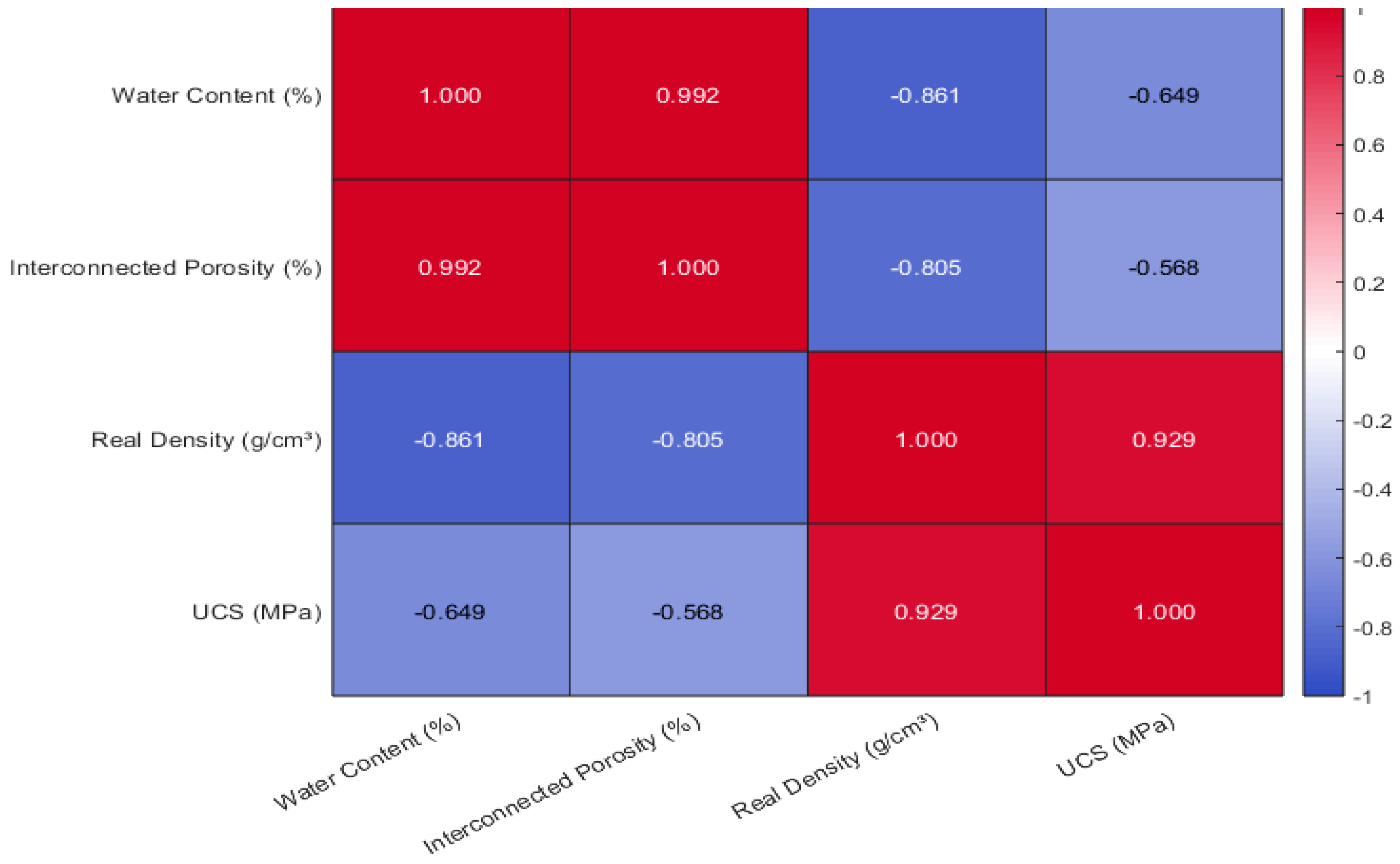
- Water Content vs. Porosity (r = 0.992): A near-perfect positive correlation indicates that specimens with higher moisture content exhibit increased interconnected porosity, reflecting the pore network’s enhanced fluid-retention capacity.
- Moisture Content vs. Real Density (r = –0.861): A strong inverse relationship indicates that specimens retaining more moisture exhibit lower density, consistent with increased pore volume reducing the mass per unit volume.
- Moisture Content vs. UCS (r = –0.649): A moderate inverse correlation indicates that higher moisture content typically reduces compressive strength, although additional factors also influence UCS variability.
- Porosity vs. Density (r = –0.805): Porosity and density are strongly inversely related, confirming that an increased void fraction corresponds to reduced material compactness.
- Porosity vs. UCS (r = –0.568): A moderate negative correlation indicates that increased porosity compromises compressive strength, underscoring pore structure as a primary weakening mechanism.
- Density vs. UCS (r = 0.929): A robust positive correlation indicates denser rocks resist compressive loading more effectively, making real density the most predictive univariate feature for UCS.
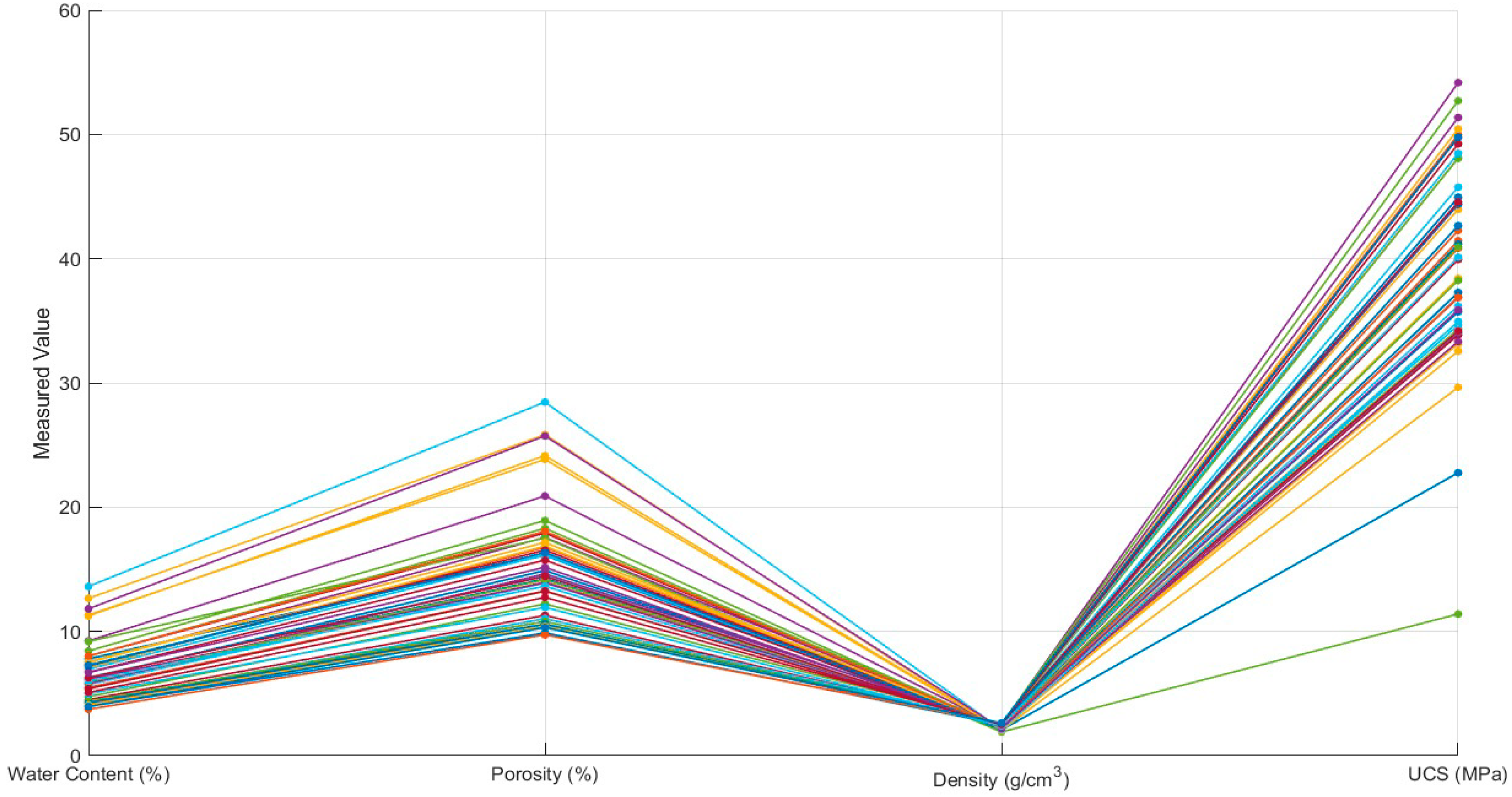
- High-strength subset (rightmost lines): Samples with UCS > 45 MPa (the upper bundle on the right axis) consistently correspond to high real density (2.5–2.7 g/cm3) and low moisture content (3–6%) and porosity (9–15%), reaffirming that dense, low-porosity rocks exhibit superior compressive resistance.
- Low-strength subset: Samples with UCS < 25 MPa align with lower real density (1.9–2.2 g/cm3) and elevated moisture content (8–14%) and porosity (18–28%), highlighting how increased pore volume and moisture compromise compressive strength.
- Intermediate cluster: The majority of samples fall within mid-range values—moisture content 5–8%, porosity 12–18%, real density 2.3–2.5 g/cm3, and UCS 30–45 MPa—reflecting the dataset’s central tendency and confirming these intervals as representative for model training.
- Outliers: A few lines diverge sharply, such as one sample with exceptionally high porosity (>25%) yet moderate UCS (~30 MPa), suggesting localized lithological variations or measurement anomalies worth further geological investigation.
6.2. Model Implementation and Training Protocols
6.2.1. Radial Basis Function (RBF) Neural Network
6.2.2. Bayesian Regularized Feed-Forward Neural Network
6.2.3. Scaled Conjugate Gradient (SCG) Neural Network
6.2.4. Levenberg–Marquardt (LM) Neural Network
6.2.5. Comparative Overview
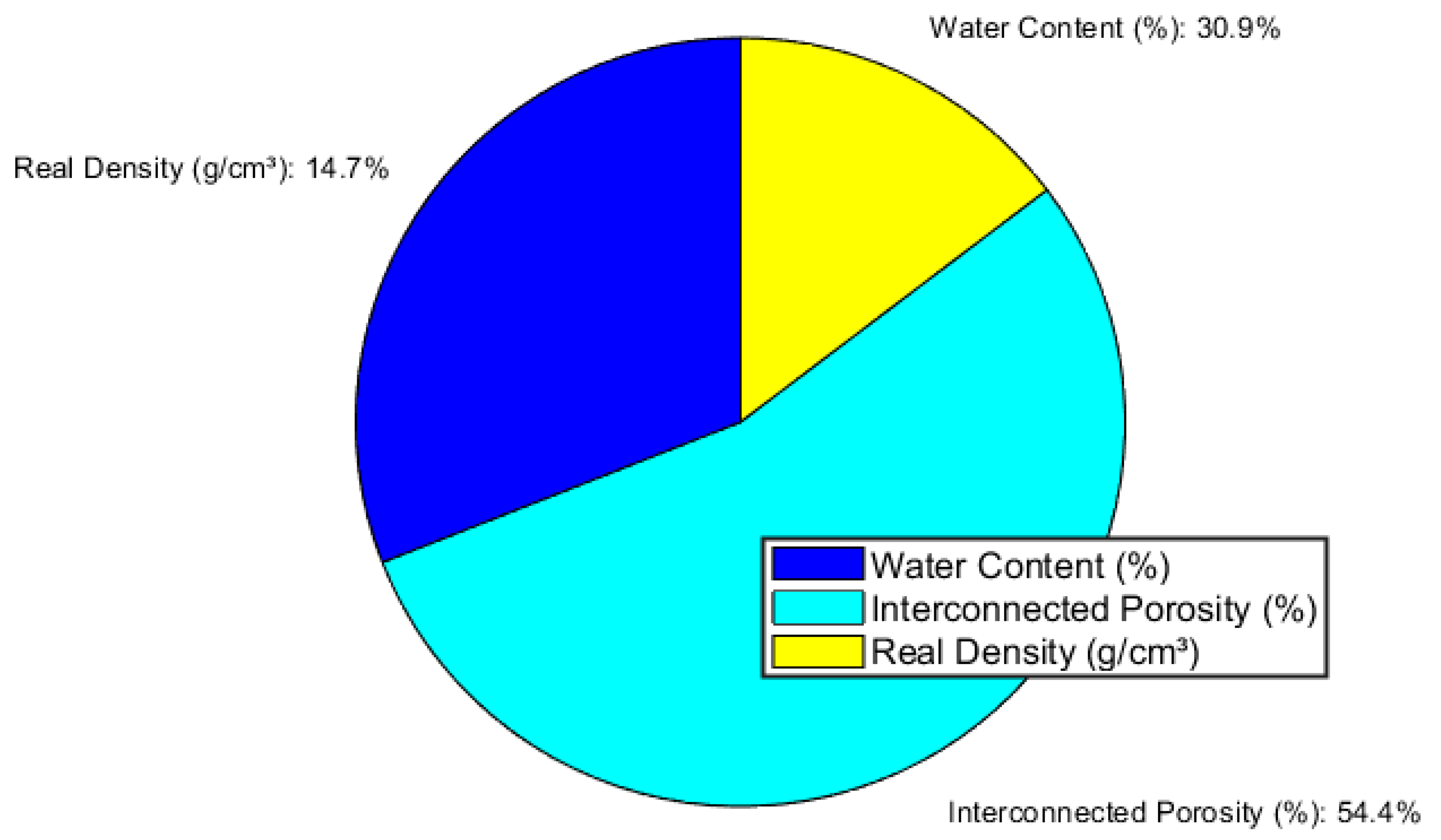
6.2.6. Sensitivity Analysis
7. Summary, Conclusions, and Future Work
7.1. Key Findings Include:
7.2. Conclusions
7.3. Future Work
Author Contributions
Funding
Institutional Review Board Statement
Informed Consent Statement
Data Availability Statement
Acknowledgments
Conflicts of Interest
References
- Peng, J.; Zhang, K. Effects of Water Content on the Mechanical Behavior of Sedimentary Rocks. Rock Mech. Rock Eng. 2007, 40, 125–137. [Google Scholar]
- Freyburg, E. The Lower and Middle Buntsandstein of Southwest Thuringia in Its Geotechnical Properties. Ger. Soc. Geosci. Ser. A 2025, 176, 911–919. [Google Scholar]
- McNally, G.H. Estimation of Coal Measures Rock Strength Using Sonic and Density Logs. Log Anal. 1987, 28, 20–27. [Google Scholar]
- Galván, M.; Restrepo, I. Nonlinear Relationships between Water Saturation and Unconfined Compressive Strength in Limestones. Int. J. Rock Mech. Min. Sci. 2016, 84, 66–74. [Google Scholar]
- Gokceoglu, C. A Comparative Study of Neural Network and Multiple Regression Analysis in Modeling Rock Properties. Eng. Geol. 2002, 66, 281–295. [Google Scholar]
- Bieniawski, Z.T. Engineering Rock Mass Classifications: A Complete Manual for Engineers and Geologists in Mining, Civil, and Petroleum Engineering; Wiley: New York, NY, USA, 1975. [Google Scholar]
- ASTM D7012-10; Standard Test Method for Compressive Strength and Elastic Moduli of Intact Rock Core Specimens Under Varying States of Stress and Temperatures. ASTM International: West Conshohocken, PA, USA, 2010.
- Naal-Pech, A. Influence of Porosity and Density on the Compressive Strength of Seybaplaya Bank Rocks. J. Geotech. Stud. 2023, 45, 215–227. [Google Scholar]
- Chang, C.; Soon, T.H.R.Y.; McDougall, S. Porosity and Compressive Strength Relationships in Carbonates. Rock Mech. Rock Eng. 2006, 39, 443–456. [Google Scholar]
- Naal-Pech, A. Extended Correlations for UCS Prediction in Karstic Limestones. In Proceedings of the 15th International Congress on Rock Mechanics, New Delhi, India, 22–27 September 2024; pp. 123–129. [Google Scholar]
- Fener, M.; Gül, E.; Ayday, O. Prediction of Uniaxial Compressive Strength Using Artificial Neural Networks. Environ. Geol. 2005, 47, 101–109. [Google Scholar]
- Naal-Pech, A.; Palemón-Arcos, L.; Gutiérrez-Can, Y.; El Hamzaoui, Y. Study of the Relationship between Uniaxial Compressive Strength vs. Non-Destructive Testing and Specific Weight in Bank Rocks from the Seybaplaya Campeche Mexico. J. Eng. Appl. 2024, 11, 16–25. [Google Scholar] [CrossRef]
- Peng, S.; Zhang, Z. Correlations of Compressive Strength (MPa) with Rock Physical Properties. Pet. Sci. 2007, 4, 67–73. [Google Scholar]
- Gokceoglu, C. A Neural Network Application to Estimate the Uniaxial Compressive Strength of Some Rocks from Their Petrographic Characteristics. Rock Mech. Rock Eng. 2002, 35, 279–293. [Google Scholar]
- Lal, R. Shale Mechanical Properties and Crack Propagation. J. Pet. Sci. 1999, 6, 235–240. [Google Scholar]
- Chang, C.; Zoback, M.D.; Khaksar, A. Empirical Relationships between Compressive Strength and Porosity in Gulf of Mexico Rocks. SPE J. 2006, 11, 19–25. [Google Scholar]
- Naal-Pech, J.W.; Palemón-Arcos, L.; El Hamzaoui, Y.; Gutiérrez-Can, Y. Study of the Relationship between Uniaxial Compressive Strength and the Point Load Test in Rocks from the Bank in Seybaplaya Campeche Mexico. J. Eng. Appl. 2024, 11, 36–42. [Google Scholar] [CrossRef]
- Wei, X.; Shahani, N.M.; Zheng, X. Predictive Modeling of the Uniaxial Compressive Strength of Rocks Using an Artificial Neural Network Approach. Mathematics 2023, 11, 1650. [Google Scholar] [CrossRef]
- Torabi-Kaveh, M.; Naseri, F.; Saneie, S.; Sarshari, B. Application of Artificial Neural Networks and Multivariate Statistics to Predict UCS and E Using Physical Properties of Asmari Limestones. Arab. J. Geosci. 2015, 8, 2889–2897. [Google Scholar] [CrossRef]
- Yagiz, S.; Sezer, E.A.; Gokceoglu, C. Artificial Neural Networks and Nonlinear Regression Techniques to Assess the Influence of Slake Durability Cycles on the Prediction of Uniaxial Compressive Strength and Modulus of Elasticity for Carbonate Rocks. Int. J. Numer. Anal. Meth. Geomech. 2012, 36, 1636–1650. [Google Scholar] [CrossRef]
- Setayeshirad, M.R.; Uromeie, A.; Nikudel, M.R. Modeling of the Uniaxial Compressive Strength of Carbonate Rocks Using Statistical Analysis and Artificial Neural Network. Rock Mech. Rock Eng. 2025. [Google Scholar] [CrossRef]
- Ceryan, N.; Okkan, U.; Kesimal, A. Prediction of Unconfined Compressive Strength of Carbonate Rocks Using Artificial Neural Networks. Environ. Earth Sci. 2013, 68, 807–819. [Google Scholar] [CrossRef]
- Abdi, Y.; Taheri-Garavand, A. Application of the ANFIS Approach for Estimating the Mechanical Properties of Sandstones. Emir. J. Eng. Res. 2020, 25, 1. [Google Scholar]
- Umrao, R.K.; Sharma, L.K.; Singh, R.; Singh, T.N. Determination of Strength and Modulus of Elasticity of Heterogeneous Sedimentary Rocks: An ANFIS Predictive Technique. Measurement 2018, 126, 194–201. [Google Scholar] [CrossRef]
- Cabalar, A.F.; Cevik, A.; Gokceoglu, C. Some Applications of Adaptive Neuro-Fuzzy Inference System (ANFIS) in Geotechnical Engineering. Comput. Geotech. 2012, 40, 14–33. [Google Scholar] [CrossRef]
- Mohamad, E.T.; Jahed Armaghani, D.; Momeni, E.; Alavi Nezhad Khalil Abad, S.V. Prediction of the Unconfined Compressive Strength of Soft Rocks: A PSO-Based ANN Approach. Bull. Eng. Geol. Environ. 2015, 74, 745–757. [Google Scholar] [CrossRef]
- Momeni, E.; Rashidi Khabir, R. A Reliable PSO-Based ANN Approach for Predicting Unconfined Compressive Strength of Sandstones. Open Constr. Build. Technol. J. 2020, 14 (Suppl. 1), 237–249. [Google Scholar] [CrossRef]
- Dehghan, S.; Sattari, G.H.; Chehreh, C.S.; Aliabadi, M.A. Prediction of Unconfined Compressive Strength and Modulus of Elasticity for Travertine Samples Using Regression and Artificial Neural Networks. Min. Sci. Technol. 2010, 20, 41–46. [Google Scholar] [CrossRef]
- Kalkan, E.; Akbulut, S.; Tortum, A.; Celik, S. Prediction of the Unconfined Compressive Strength of Compacted Granular Soils by Using Inference Systems. Environ. Geol. 2009, 58, 1429–1440. [Google Scholar] [CrossRef]
- Baykaşoğlu, A.; Güllü, H.; Çanakçı, H.; Özbakır, L. Prediction of Compressive and Tensile Strength of Limestone via Genetic Programming. Expert Syst. Appl. 2008, 35, 111–123. [Google Scholar] [CrossRef]
- Xue, X.; Wei, Y. A Hybrid Modelling Approach for Prediction of Uniaxial Compressive Strength of Rock Materials. C. R. Mécanique 2020, 348, 235–243. [Google Scholar] [CrossRef]
- Gokceoglu, C.; Zorlu, K. A Fuzzy Model to Predict the Uniaxial Compressive Strength and the Modulus of Elasticity of a Problematic Rock. Eng. Appl. Artif. Intell. 2004, 17, 61–72. [Google Scholar] [CrossRef]
- Khatti, J.; Grover, K.S. Estimation of Intact Rock Uniaxial Compressive Strength Using Advanced Machine Learning. Transp. Infrastruct. Geotechnol. 2024, 11, 1989–2022. [Google Scholar] [CrossRef]
- Sabri, M.S.; Jaiswal, A.; Verma, A.K.; Singh, T.N. Advanced Machine Learning Approaches for Uniaxial Compressive Strength Prediction of Indian Rocks Using Petrographic Properties. Multiscale Multidiscip. Model. Exp. Des. 2024, 7, 5265–5286. [Google Scholar] [CrossRef]
- Kochukrishnan, S.; Krishnamurthy, P.; Yuvarajan, D.; Kaliappan, N. Comprehensive Study on the Python-Based Regression Machine Learning Models for Prediction of Uniaxial Compressive Strength Using Multiple Parameters in Charnockite Rocks. Sci. Rep. 2024, 14, 7360. [Google Scholar] [CrossRef] [PubMed]
- Servicio Geológico Mexicano. Implementing the 1992 Mining Law: Analysis of Mineral Substances and Administration of Concessions; Servicio Geológico Mexicano: Mexico City, Mexico, 2021. [Google Scholar]
- ASTM D4543-12; Standard Practices for Preparing Rock Core as Cylindrical Test Specimens and Verifying Conformance to Dimensional and Shape Tolerances. ASTM International: West Conshohocken, PA, USA, 2012.
- ASTM D7012-23; Standard Test Methods for Compressive Strength and Elastic Moduli of Intact Rock Core Specimens under Varying States of Stress and Temperatures. ASTM International: West Conshohocken, PA, USA, 2023.
- ASTM D2216-10; Standard Test Methods for Laboratory Determination of Water (Moisture) Content of Soil and Rock by Mass. ASTM International: West Conshohocken, PA, USA, 2010.
- ASTM D854-23; Standard Test Methods for Specific Gravity of Soil Solids by the Water Displacement Method. ASTM International: West Conshohocken, PA, USA, 2023.
- ASTM D4404-18; Standard Test Method for Determination of Pore Volume and Pore Volume Distribution of Soil and Rock by Mercury Intrusion Porosimetry. ASTM International: West Conshohocken, PA, USA, 2018.
- Nieto, G.C.; Avendaño, D.P. Laboratory Guide for Material Strength Testing; Inimagdalena: Bogotá, Colombia, 2015. [Google Scholar]
- Naal-Pech, J.W.; Palemón-Arcos, L.; El Hamzaoui, Y.; Gutiérrez-Can, Y. Study of the Relationship between Uniaxial Compressive Strength, Water Content, Porosity and Density in Bank Rocks in Seybaplaya Campeche. J. Mech. Eng. 2023, 7, 9–16. [Google Scholar] [CrossRef]
- Moody, C.J.C.H.; Darken, C.J. Fast Learning in Networks of Locally-Tuned Processing Units. Neural Comput. 1989, 1, 281–294. [Google Scholar] [CrossRef]
- MacKay, D.J.C. Bayesian Interpolation. Neural Comput. 1992, 4, 415–447. [Google Scholar] [CrossRef]
- Møller, M.F. A Scaled Conjugate Gradient Algorithm for Fast Supervised Learning. Neural Netw. 1993, 6, 525–533. [Google Scholar] [CrossRef]
- Hagan, M.T.; Menhaj, M.R. Training Feedforward Networks with the Marquardt Algorithm. IEEE Trans. Neural Netw. 1994, 5, 989–993. [Google Scholar] [CrossRef]
- Uzuner, S.; Cekmecelioğlu, D. Comparison of Artificial Neural Networks (ANN) and Adaptive Neuro-Fuzzy Inference System (ANFIS) Models in Simulating Polygalacturonase Production. BioResources 2016, 11, 8676–8685. [Google Scholar] [CrossRef]
- Sada, S.O.; Ikpeseni, S.C. Evaluation of ANN and ANFIS Modeling Ability in the Prediction of AISI 1050 Steel Machining Performance. Heliyon 2021, 7, e06136. [Google Scholar] [CrossRef]
- Zhang, G.; Patuwo, B.E.; Hu, M.Y. Forecasting with Artificial Neural Networks: The State of the Art. Int. J. Forecast. 1998, 14, 35–62. [Google Scholar] [CrossRef]
- Chong, D.J.S.; Chan, Y.J.; Arumugasamy, S.K.; Yazdi, S.K.; Lim, J.W. Optimisation and Performance Evaluation of Response Surface Methodology (RSM), Artificial Neural Network (ANN) and Adaptive Neuro-Fuzzy Inference System (ANFIS) in the Prediction of Biogas Production from Palm Oil Mill Effluent (POME). Energy 2023, 266, 126449. [Google Scholar] [CrossRef]
- Friedman, J.H. Multivariate Adaptive Regression Splines. Ann. Stat. 1991, 19, 1–67. [Google Scholar] [CrossRef]
- Dimopoulos, I.; Bourret, P.; Lek, S. Use of Some Sensitivity Criteria for Choosing Networks with Good Generalization Ability. Neural Process. Lett. 1995, 2, 1–4. [Google Scholar] [CrossRef]


| Sample Range | UTM Coordinates (X, Y) |
|---|---|
| Samples 1–10 | (741595, 2174717) |
| Samples 11–20 | (741611, 2174838) |
| Samples 21–30 | (741585, 2174851) |
| Samples 31–40 | (741591, 2174750) |
| Samples 41–50 | (741605, 2174803) |
| Water Content | Interconnected Porosity | Real Density | UCS | |
|---|---|---|---|---|
| Mean | 6.707 | 15.459 | 2.352 | 40.14 |
| Std_dev | 2.335 | 4.377 | 0.159 | 7.914 |
| Min | 3.73 | 9.73 | 1.91 | 11.4 |
| 1st_quartile | 5.0 | 12.35 | 2.262 | 34.932 |
| Median | 6.235 | 14.565 | 2.355 | 40.485 |
| 3rd_quartile | 7.552 | 17.168 | 2.478 | 44.845 |
| Max | 13.62 | 28.46 | 2.62 | 54.17 |
| Model | MATLAB Function | Topology | Data Split | Preprocessing | Key Hyperparameters | Performance Metrics |
|---|---|---|---|---|---|---|
| RBF network | newrb | Up to 25 Gaussian units | 80% train/20% test | Inputs z-score; outputs mapminmax [0,1] | Spread = 0.8; goal MSE = 1 × 10⁻³ | RMSE, R2 |
| Bayesian regularized NN | trainbr | 1 hidden layer, 15 neurons | 80%/20% | z-score; mapminmax | Max epochs = 1 000; α, β auto-tuned | MAE, COD |
| SCG network | trainscg | 1 hidden layer, 15 neurons | 70%/15%/15% | z-score; mapminmax | λ0 = 1.0 × 10⁻³;σ = 1.0 × 10⁻⁶; reg = 0.01 | RMSE, MAPE |
| LM network | trainlm | 1 hidden layer, 15 neurons | 70%/15%/15% | z-score; mapminmax | μ0 = 1.0 × 10⁻³; μ↓ = 0.1; μ↑ = 10; reg = 0.1 | COD, RMSE |
| Algorithm | R2 | RMSE (MPa) | MAE (MPa) |
|---|---|---|---|
| RBF neural network | 0.972 | 1.313 | 1.029 |
| Bayesian regularized neural network | 0.967 | 1.413 | 1.164 |
| Scaled conjugate gradient neural network | 0.964 | 1.49 | 1.264 |
| Levenberg–Marquardt neural network | 0.951 | 1.737 | 1.453 |
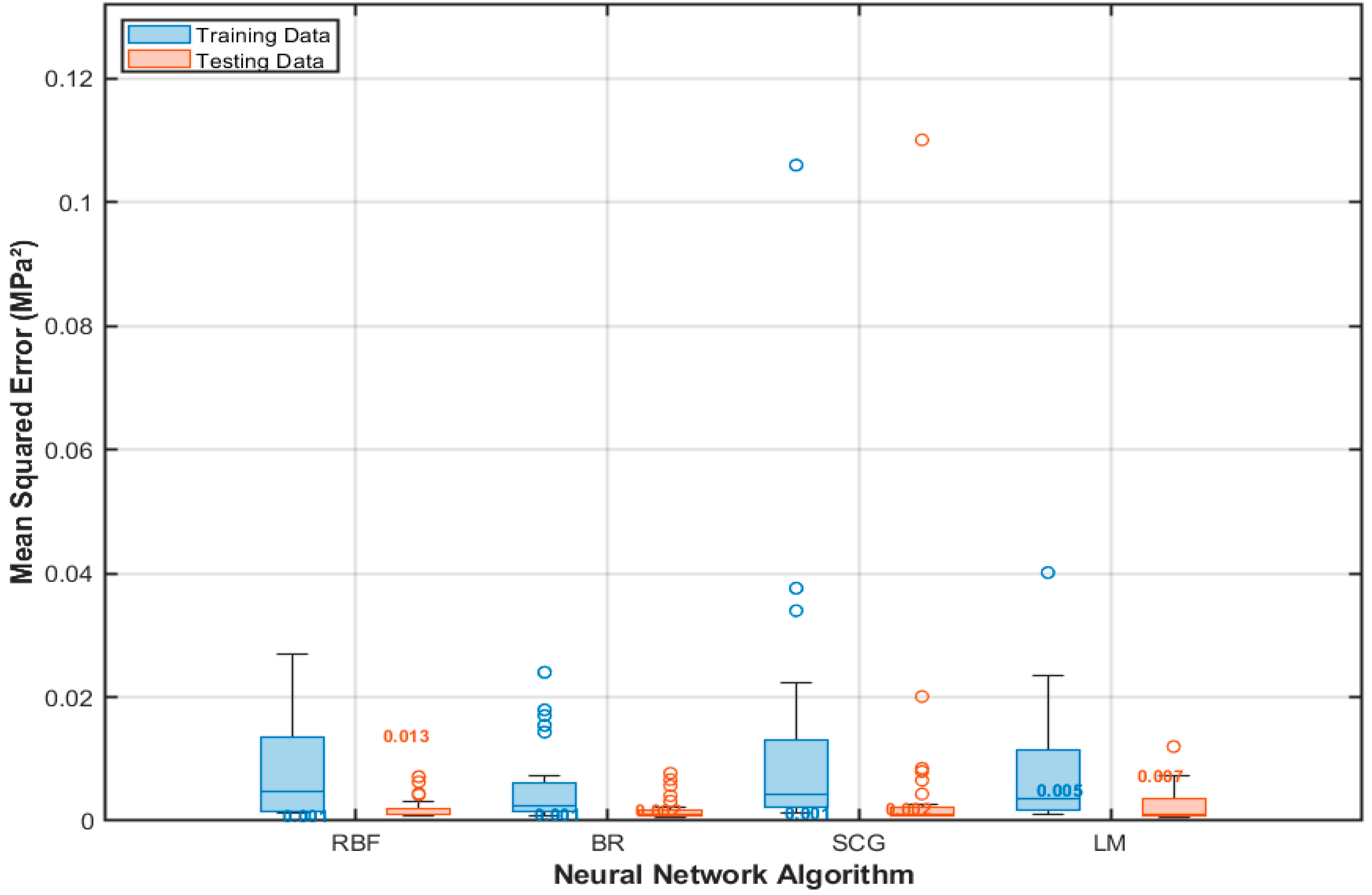
| Algorithm | Median MSE_Train | Median MSE_Test |
|---|---|---|
| RBF | 0.0008 | 0.0128 |
| Bayesian | 0.0010 | 0.0017 |
| SCG | 0.0013 | 0.0019 |
| LM | 0.0046 | 0.0068 |
| Comparison | p-Value | Adjusted (p) Significant |
|---|---|---|
| RBF vs. BR | 0.000012 | 0.000037 * |
| RBF vs. SCG | 0.000002 | 0.000010 * |
| RBF vs. LM | 0.130592 | 0.156710 * |
| BR vs. SCG | 0.599936 | 0.599936 |
| BR vs. LM | 0.000136 | 0.000204 * |
| SCG vs. LM | 0.000082 | 0.000164 * |
| Algorithm | Median R2_Train | Median R2_Test |
|---|---|---|
| RBF | 0.9753 | 0.5932 |
| Bayesian | 0.9690 | 0.9286 |
| SCG | 0.9575 | 0.9274 |
| LM | 0.8532 | 0.8043 |
| Comparison | p-Value | Adjusted (p) Significant |
|---|---|---|
| RBF vs. BR | 0.000006 | 0.000017 * |
| RBF vs. SCG | 0.000002 | 0.000010 * |
| RBF vs. LM | 0.059836 | 0.071803 |
| BR vs. SCG | 0.530440 | 0.530440 |
| BR vs. LM | 0.000075 | 0.000113 * |
| SCG vs. LM | 0.000063 | 0.000113 * |
Disclaimer/Publisher’s Note: The statements, opinions and data contained in all publications are solely those of the individual author(s) and contributor(s) and not of MDPI and/or the editor(s). MDPI and/or the editor(s) disclaim responsibility for any injury to people or property resulting from any ideas, methods, instructions or products referred to in the content. |
© 2025 by the authors. Licensee MDPI, Basel, Switzerland. This article is an open access article distributed under the terms and conditions of the Creative Commons Attribution (CC BY) license (https://creativecommons.org/licenses/by/4.0/).
Share and Cite
Naal-Pech, J.W.; Palemón-Arcos, L.; El Hamzaoui, Y. Comparative Evaluation of Feed-Forward Neural Networks for Predicting Uniaxial Compressive Strength of Seybaplaya Carbonate Rock Cores. Appl. Sci. 2025, 15, 5609. https://doi.org/10.3390/app15105609
Naal-Pech JW, Palemón-Arcos L, El Hamzaoui Y. Comparative Evaluation of Feed-Forward Neural Networks for Predicting Uniaxial Compressive Strength of Seybaplaya Carbonate Rock Cores. Applied Sciences. 2025; 15(10):5609. https://doi.org/10.3390/app15105609
Chicago/Turabian StyleNaal-Pech, Jose W., Leonardo Palemón-Arcos, and Youness El Hamzaoui. 2025. "Comparative Evaluation of Feed-Forward Neural Networks for Predicting Uniaxial Compressive Strength of Seybaplaya Carbonate Rock Cores" Applied Sciences 15, no. 10: 5609. https://doi.org/10.3390/app15105609
APA StyleNaal-Pech, J. W., Palemón-Arcos, L., & El Hamzaoui, Y. (2025). Comparative Evaluation of Feed-Forward Neural Networks for Predicting Uniaxial Compressive Strength of Seybaplaya Carbonate Rock Cores. Applied Sciences, 15(10), 5609. https://doi.org/10.3390/app15105609