Salp Swarm Algorithm Optimized A* Algorithm and Improved B-Spline Interpolation in Path Planning

Abstract

The efficiency and smoothness of path planning algorithms are critical factors influencing their practical applications. A traditional A* algorithm suffers from limitations in search efficiency, path smoothness, and obstacle avoidance. To address these challenges, this paper introduces an improved A* algorithm that integrates the Salp Swarm Algorithm (SSA) for heuristic function optimization and proposes a refined B-spline interpolation method for path smoothing. The first major improvement involves enhancing the A* algorithm by optimizing its heuristic function through the SSA. The heuristic function combines Chebyshev distance, Euclidean distance, and obstacle density, with the SSA adjusting the weight parameters to maximize efficiency. The simulation experimental results demonstrate that this modification reduces the number of searched nodes by more than 78.2% and decreases planning time by over 48.1% compared to traditional A* algorithms. The second key contribution is an improved B-spline interpolation method incorporating a two-stage optimization strategy for smoother and safer paths. A corner avoidance strategy first adjusts control points near sharp turns to prevent collisions, followed by a path obstacle avoidance strategy that fine-tunes control point positions to ensure safe distances from obstacles. The simulation experimental results show that the optimized path increases the minimum obstacle distance by 0.2–0.5 units, improves the average distance by over 43.0%, and reduces path curvature by approximately 61.8%. Comparative evaluations across diverse environments confirm the superiority of the proposed method in computational efficiency, path smoothness, and safety. This study presents an effective and robust solution for path planning in complex scenarios.

1. Introduction

Path planning [1] is a fundamental technology for robotic navigation and autonomous driving, with its performance directly determining the efficiency and safety of mobile agents. The algorithm must generate optimal and smooth collision-free paths to reduce collision risks. Path planning [2] focuses on discovering an optimal trajectory that avoids obstacles between a starting point and a destination. An ideal path planning algorithm needs to meet two key requirements: first, it must be computationally efficient, capable of generating feasible paths in real time; second, the generated path must be smooth and safe for practical execution.

Path planning algorithms can be broadly classified into two types: global path planning and local path planning. Currently, common global path planning algorithms include graph search-based algorithms, sampling-based algorithms, intelligent optimization algorithms, mathematical model-based algorithms, and hybrid algorithms. Graph search-based algorithms include Dijkstra’s Algorithm [3], A* algorithms [4], and hybrid A* algorithms [5]. Sampling-based algorithms include the Rapidly Exploring Random Tree (RRT) algorithm [6] and RRT* algorithm [7]. Intelligent optimization algorithms include the Genetic Algorithm [8], Ant Colony Optimization (ACO) [9], and Particle Swarm Optimization (PSO) [10]. Mathematical model-based algorithms include the Dynamic Programming (DP) algorithm [11]. Hybrid algorithms [12] combine the advantages of multiple algorithms to improve path quality and search efficiency. The Intelligent Bug algorithm [13] and its variants are currently the most commonly used methods for solving local path planning problems. Among these path planning algorithms, the A* algorithm is recognized as one of the most efficient direct search methods for solving the shortest path in static road networks. Due to its balance of optimality and efficiency [14], it has been widely used.

The A* algorithm combines Dijkstra’s comprehensive search with heuristic guidance, greatly reducing unnecessary node expansion and improving search efficiency. However, as more scholars have delved into the A* algorithm, several drawbacks have been identified, such as the generation of non-smooth paths and a decrease in search efficiency when the map size increases. Over the years, both domestic and international scholars have made various improvements to the A* algorithm. Common optimization strategies include improving the heuristic function, enhancing the search neighborhood, and modifying the search strategy. Wu et al. [15] proposed a heuristic function mechanism with directional information, which enhances the algorithm’s directional intelligence, helping to reduce computational complexity and time. Zheng et al. [16] introduced the DPIO method, which optimizes the heuristic function to enhance the efficiency and quality of path planning. Zhang et al. [17] optimized the heuristic function and introduced the Jump Point Search strategy, reducing the number of nodes that need to be expanded during the path search process, thus improving the algorithm’s efficiency and reducing computational time and memory consumption. Huang et al. [18] proposed a new 5-neighborhood search method, dynamically adjusting the search neighborhood (5-neighborhood, 4-neighborhood, or 3-neighborhood) based on obstacle constraints, thereby improving path smoothness.

Among the aforementioned algorithms, the A* algorithm has shown improvements in both search efficiency and path smoothness. However, these improvements, due to the need for dynamic adaptation, can consume considerable computer resources. Additionally, the Jump Point Search strategy may not effectively handle dense obstacle environments in certain cases. In recent years, with the rapid development of intelligent optimization algorithms, various swarm intelligence optimization algorithms such as the Salp Swarm Algorithm (SSA) [19], Bobcat Optimization Algorithm [20], and Wombat Optimization Algorithm [21] have demonstrated remarkable advantages in the field of path planning due to their excellent global search capabilities and convergence performance. These algorithms, by simulating the intelligent behaviors of biological groups in nature, provide novel approaches for solving complex optimization problems. Therefore, this paper proposes an improved A* algorithm based on the SSA. The algorithm introduces a new A* heuristic function and optimizes its weight coefficients to enhance search efficiency while ensuring path feasibility. Furthermore, this paper also optimizes path smoothing to enhance the safety and smoothness of the final path.

In practical applications, path smoothing is crucial. Traditional path smoothing methods include the Artificial Potential Field [22], Bezier curves [23], and B-spline interpolation [24], and others. Among these, the B-spline interpolation algorithm is the most widely applied. However, traditional methods like B-spline interpolation often struggle to maintain a safe distance from obstacles. To address this, our approach integrates an obstacle avoidance mechanism into the smoothing process, balancing both path smoothness and safety. We propose a two-stage optimized B-spline interpolation strategy: in the first stage, control point positions are adjusted to avoid collisions with obstacles; in the second stage, global obstacle avoidance is achieved.

In conclusion, this paper focuses on how to optimize the A* algorithm using the SSA to improve the efficiency of path search and proposes an improved B-spline smoothing strategy to guarantee the safety and smoothness of the path. The following chapters will provide a comprehensive explanation of the proposed method, followed by the experimental results and comparative analysis to validate the effectiveness of the proposed approach.

The main structure of this paper is as follows: Section 2 introduces the path planning algorithm, proposing an A* algorithm optimized by the SSA. Section 3 elaborates on the path smoothing algorithm, presenting an improvement of the B-spline interpolation method. The simulation experiments of the two proposed algorithms are demonstrated in Section 4. The conclusions are given in Section 5.

2. Path Planning Algorithm

2.1. The A* Algorithm

The A* algorithm is a heuristic search algorithm proposed by Peter Hart et al. in 1968 [25]. It combines the optimality guarantee of Dijkstra’s Algorithm with the efficiency of greedy search. Unlike traditional non-heuristic search methods, the A* algorithm considers both the estimated distance from the current node to the target and the actual cost to reach the node while exploring the path. A combined priority score, $f\left(n\right)=g\left(n\right)+h\left(n\right)$, is computed to intelligently guide the search process. This mechanism enables the A* algorithm to ensure optimal solutions while significantly improving search efficiency, which is why it has been broadly utilized in various fields such as path planning, game AI, and robot navigation.

However, despite its excellent performance in many scenarios, the A* algorithm still has some limitations. First, its computational time can be long, particularly in large maps where the algorithm must expand a large number of nodes and maintain open and closed lists, which increases the computational burden significantly. Second, the performance of the A* algorithm is critically determined by the design of the heuristic function $h\left(n\right)$. If the heuristic function is unacceptable or inconsistent, the algorithm may fail to find the optimal solution or experience a significant drop in efficiency.

2.2. Improvement of the A* Algorithm

To address the limitations of the traditional A* algorithm and considering that its performance is highly dependent on the design of the heuristic function $h\left(n\right)$, it is important to recognize that the heuristic function not only determines whether the algorithm can find the optimal solution, but also directly affects the search efficiency. The traditional A* algorithm imposes a strict requirement on the heuristic function $h\left(n\right)$, which must satisfy $h\left(n\right)\le the actual minimum cost$. This condition guarantees that the algorithm is capable of identifying the shortest possible path; however, it also leads to the expansion of a large number of nodes, resulting in longer computation times. In practical applications, once path planning is completed, the path is often smoothed, a process that may increase the path length. Therefore, during the initial phase of path planning, there is no need to strictly pursue the shortest path, but rather, it is more practical to seek a balance between path quality and computational efficiency.

Based on this understanding, this chapter proposes an improvement strategy: by relaxing the strict requirements on the shortest path, we attempt to construct a new heuristic function, making the A* algorithm no longer focus solely on minimizing the distance. This approach significantly improves the algorithm’s computational efficiency while ensuring the path remains reasonable. This improvement not only reduces the number of nodes expanded by the algorithm and alleviates the computational burden, but also better accommodates the flexible requirements of path planning in real-world applications. To validate this hypothesis, we designed and implemented a new heuristic function and further improved it using the SSA. We refer to this algorithm as the SSA-A*.

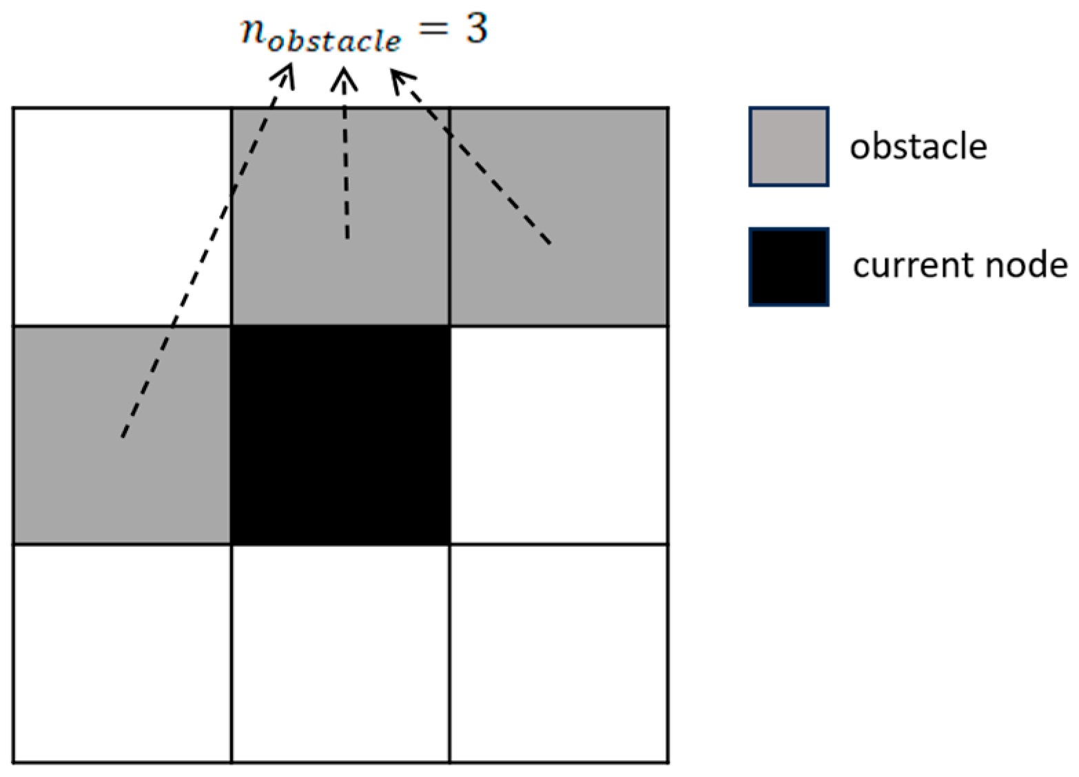
2.2.1. Determining the Variables Included in $h\left(n\right)$

First, it is necessary to identify the variables in $h\left(n\right)$. For an eight-directional search, the traditional A* algorithm’s heuristic function $h\left(n\right)$ often utilizes either the Chebyshev distance or the Euclidean distance. Among these, the Chebyshev distance is more effective in measuring the number of moves in an eight-directional grid, while the Euclidean distance better represents the actual distance. Therefore, we use both distance metrics simultaneously to enhance the accuracy of the heuristic function $h\left(n\right)$ in distance evaluation.

Additionally, considering that when a node is surrounded by many obstacles, the path passing through that node may increase in length due to the need to avoid obstacles, we also incorporate the obstacle density into the heuristic function $h\left(n\right)$. This addition enables the search process to possess a certain level of obstacle avoidance capability.

Thus, we modify the heuristic function $h\left(n\right)$ as follows (1):

$$\left\{\begin{array}{c}h\left(n\right)={\omega }_1\ast d_{Chebyshev}+{\omega }_2\ast d_{Euclidean}+{\omega }_3\ast {\rho }_{obstacle}\\ {\rho }_{Obstacle}={\displaystyle \frac{n_{obstacle}}{8}}\end{array}\right.$$

(1)

In this context, $d_{Chebyshev}$ represents the Chebyshev distance from the current node $n$ to the goal node, $d_{Euclidean}$ denotes the Euclidean distance, ${\rho }_{obstacle}$ represents the obstacle density in the 8-neighborhood of the current node $n$, and $n_{obstacle}$ refers to the number of obstacles in the 8-neighborhood of node $n$ (as illustrated in Figure 1). ${\omega }_1,{\omega }_2,{\omega }_3$ are weight coefficients.

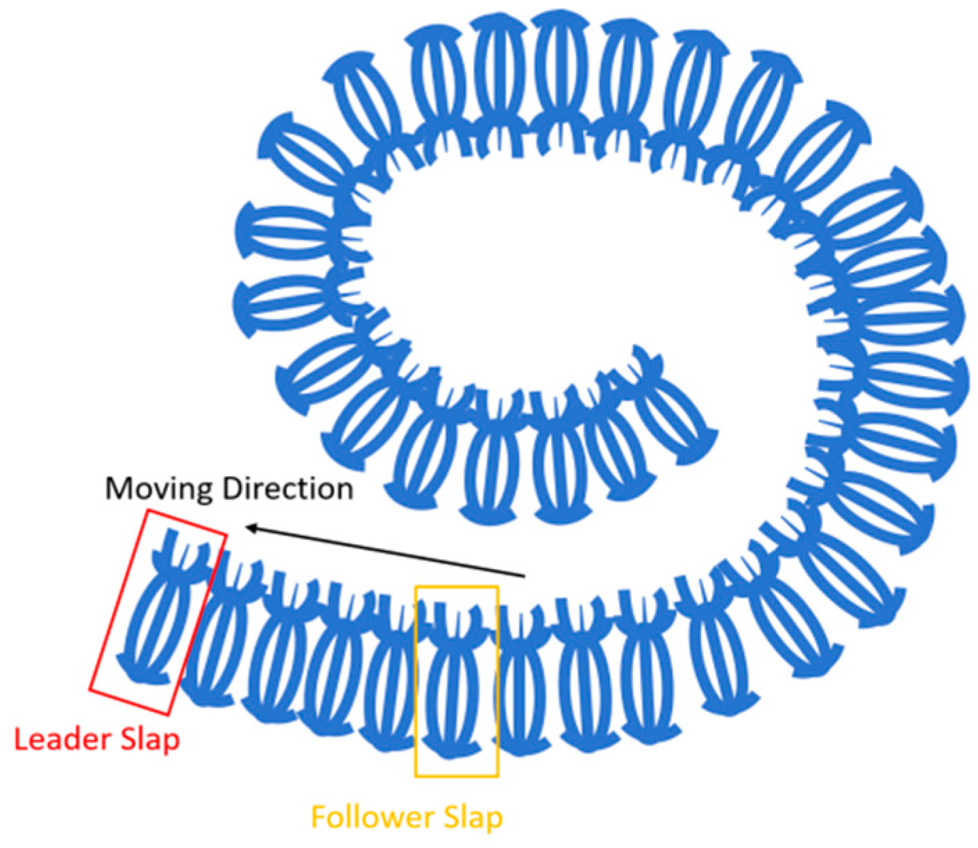
2.2.2. Optimization Using the SSA

To determine the weight coefficients ${\omega }_1,{\omega }_2,{\omega }_3$, an efficient optimization method is required. The combination of these weight coefficients directly impacts the performance of the heuristic function, and therefore, identifying the optimal solution in a complex parameter space is of critical importance.

When selecting an optimization method, we take into account that the optimization problem for the weight coefficients may have multiple local optima. Thus, an algorithm that can effectively prevent being trapped in local optima is required. Moreover, to enhance optimization efficiency, the algorithm should be able to find a near-optimal solution in fewer iterations. Additionally, the algorithm needs to handle nonlinear, multi-modal optimization problems to accommodate the complexity of the weight coefficients in the heuristic function, and it should be easy to implement and insensitive to initial parameter settings, reducing the complexity of tuning. Based on these requirements, we have chosen the SSA for the optimization of the weight coefficients.

The Salp Swarm Algorithm (SSA) [26], proposed by Seyedali Mirjalili et al. [27] in 2017, is a nature-inspired swarm intelligence algorithm that simulates the foraging behavior of salps (as shown in Figure 2). Salps are marine organisms that search for food through collective cooperation and leader-following behavior. The SSA leverages this behavior to optimize problem solutions. Salps form chain-like swarms in the ocean, and the SSA simulates this behavior by dividing the swarm into leaders and followers. The leader is at the front of the chain and is responsible for guiding the group, while the followers move by following the leader. The SSA simulates the foraging behavior of salp swarms in the ocean, offering strong global search capability and efficiently exploring high-dimensional parameter spaces [28]. Its rapid convergence speed makes it suitable for solving complex optimization problems. Furthermore, the SSA is insensitive to initial parameter settings, simple to implement, and easy to adjust, making it well suited to meet our optimization needs.

Next, the SSA is used to determine the weight coefficients ${\omega }_1,{\omega }_2,{\omega }_3$. First, we initialize the population using (2) and (3).

$$x=\left[\begin{array}{c}\begin{array}{cccc}{X}_1^1& X_2^1& \dots & X_d^1\\ X_1^2& X_2^2& \dots & X_d^2\\ ⋮& ⋮& \ddots & ⋮\end{array}\\ \begin{array}{cccc}{X}_1^n& X_2^n& \dots & X_d^n\end{array}\end{array}\right]$$

(2)

$$X_j^i=rand\ast \left(u{b}_j-l{b}_j\right)+l{b}_j,i\in \left\{1,2,\dots ,n\right\},j\in \left\{1,2,\dots ,n\right\}$$

(3)

$X$ is an $n\ast d$ matrix, with $n$ representing the population size and $d$ representing the dimensionality of the problem. The terms $ub$ and $lb$ denote the upper and lower bounds of the problem, respectively, while $rand$ is a randomly generated number between $0$ and $1$.

To enhance the efficiency of the A* algorithm, we define the fitness function as the number of searched nodes, where a lower number of searched nodes indicates a higher fitness score. Each individual’s fitness is ranked, with the highest fitness individual designated as the leader and the remaining individuals as followers. Subsequently, both the leader and followers update their positions according to the predefined formulas. The leader’s position is updated using (4) and (5).

$$X_j^i=\left\{\begin{array}{c}{F}_j+c_1\left[\left(u{b}_j-l{b}_j\right)\ast c_2+l{b}_j\right],c_3\le 0.5\\ F_j-c_1\left[\left(u{b}_j-l{b}_j\right)\ast c_2+l{b}_j\right],c_3>0.5\end{array}\right.$$

(4)

$$c_1=2e^{-{\left({\displaystyle \frac{4t}{T}}\right)}^2}$$

(5)

The followers update their positions using (6).

$$X_j^i={\displaystyle \frac{1}{2}}\left(X_j^i+X_j^{i-1}\right)$$

(6)

After each update, the fitness of each individual is re-evaluated, and the optimization process iterates until a predefined number of iterations is reached or a convergence criterion is met. Finally, the optimal weight parameters are selected. Using these optimal weight parameters, the heuristic function $h\left(n\right)$ is determined and subsequently employed for path planning.

The pseudo-code for the optimization of the A* algorithm using the SSA is shown in Algorithm 1 below.

Algorithm 1: Improved A* Algorithm with the SSA Optimization

Input: Grid map $G$, start point $S$, end point $E$, weight bounds ${\Omega }_{bounds}$, population size $N$, maximum iterations $T$ Output: Optimal path $P$, visited nodes list $V$, optimal weight ${\Omega }^{\ast }$ 1: BEGIN: 2: Initialization:     Define 8-neighborhood direction set      $D=\left\{\left(-1,0\right),\left(1,0\right),\left(0,-1\right),\left(0,1\right),\left(-1,-1\right),\left(-1,1\right),\left(1,-1\right),\left(1,1\right)\right\}$     Initialize SSA population $P=\left\{{\Omega }_i\mid {\Omega }_i\sim Uniform\left({\Omega }_{bounds}\right),i=1,2,\dots ,N\right\}$     Initialize optimal weight ${\Omega }^{\ast }\leftarrow argmi{n}_{\Omega \in P}Fitness\left(\Omega \right)$     Initialize optimal fitness $F^{\ast }\leftarrow Fitness\left({\Omega }^{\ast }\right)$     Initialize iteration counter $t\leftarrow 0$ 3://SSA Optimization Process: 4: While $t<T$: 5:    For each ${\Omega }_i\in P:$ 6:     If $Random()<0.5:$ 7:      ${{\Omega }_i}^{\prime }\leftarrow {\Omega }^{\ast }+Uniform{\left(-0.3,0.3\right)}^3$ 8:     Else: 9:      ${{\Omega }_i}^{\prime }\leftarrow {\displaystyle \frac{{\Omega }_i+{\Omega }^{\ast }}{2}}$ 10:     Clip ${\Omega }_i$ to ${\Omega }_{bounds}$ 11:     ${Fi}^{\prime }\leftarrow Fitness\left({\Omega }_i\prime \right)$ 12:     If${Fi}^{\prime }<F^{\ast }:$ 13:      ${\Omega }^{\ast }\leftarrow {{\Omega }_i}^{\prime }$ 14:      $F^{\ast }\leftarrow {F_i}^{\prime }$ 15:      $P\leftarrow \left\{{{\Omega }_i}^{\prime }\right\}$ 16:    Record current optimal fitness $F^{\ast }$ 17:    $t\leftarrow t+1$ 18: //A* Path Search:Use optimal weight Ω∗ to execute A* algorithm: 19: Initialize open list $O\leftarrow \left\{\left(f\left(S\right),0,S\right)\right\}$, parent map $C\leftarrow \left\{\right\}$, cost map $G\leftarrow \left\{S:0\right\}$, and visited nodes list $V\leftarrow []$ 20: While $O$ is not empty: 22:    Pop $\left(f,g,Q\right)\leftarrow HeapPop\left(O\right)$ 23:    If $Q=E:$ 24:     $P\leftarrow ReconstructPath\left(C,S,E\right)$ 25:     Return $P,V$ 26:    Add $Q$ to $V$ 27:    For each $\left(dx,dy\right)\in D:$ 28:     $Q^{\prime }\leftarrow \left(Q_x+dx,Q_y+dy\right)$ 29:     If $Q^{\prime }$ is out of bounds or $G\left[Q^{\prime }\right]=1:$ 30:      Continue 31:     $c\leftarrow DiagonalDistance$ if $\mid dx\mid +\mid dy\mid =2else1$ 32:     $g^{\prime }\leftarrow g+c$ 33:     If $Q^{\prime }\notin Gor{g}^{\prime }<G\left[Q^{\prime }\right]:$ 34:      $G\left[Q^{\prime }\right]\leftarrow g$ 35:      $C\left[Q^{\prime }\right]\leftarrow Q$ 36:      $h\leftarrow Heuristic\left(Q^{\prime },E,{\Omega }^{\ast },G\right)$ 37:      $f^{\prime }\leftarrow g^{\prime }+h$ 38:      Push $\left(f^{\prime },g^{\prime },Q^{\prime }\right)$ into $O$ 39: Return $None,V$ 40: END

Our work, compared with recent SSA-based path planning studies, demonstrates distinct focuses and innovations. Our proposed algorithm employs SSA to optimize the heuristic function weights of the A* algorithm, dynamically adjusting the weights by incorporating Chebyshev distance, Euclidean distance, and obstacle density to enhance search efficiency. Guo et al. [29] improved the SSA for AUV path planning by introducing the Levy flight strategy and a nonlinear convergence factor to boost the algorithm’s global search capability and convergence speed. Meanwhile, Mohammad AlShabi et al. [30] applied SSA to ground vehicle path planning, exploring a new application scenario for the algorithm.

3. Path Smoothing Algorithm

3.1. B-Spline Interpolation Curve

B-spline is a mathematical method commonly used in computer graphics and data fitting. It consists of a series of control points, knot vectors, and a set of basis functions. The control points determine the shape of the spline curve, allowing shape adjustments by repositioning them. The knot vector defines the distribution of the spline curve in parameter space and determines the influence range of each control point on the spline curve. The algorithm utilizes a set of basis functions to construct the spline curve. By weighting the control points with the corresponding basis functions, a smooth interpolated curve can be obtained. The basis functions are computed using a recursive formula, defined as (7) and (8).

$$k=0,B_{i,0}\left(t\right)=\left\{\begin{array}{c}1, t_i\le t\le t_{i+1}\\ 0, Otherwise\end{array}\right.$$

(7)

$$k>1,B_{i,k}\left(t\right)={\displaystyle \frac{t-t_i}{t_{i+k}-t_i}} B_{i,k-1}\left(t\right)+{\displaystyle \frac{t_{i+k+1}-t}{t_{i+k+1}-t_{i+1}}} B_{i+1,k-1}\left(t\right)$$

(8)

The mathematical formula of the B-spline curve is typically expressed as (9).

$$P\left(t\right)={\displaystyle \sum }_{i=0}^n{P}_i{B}_{i,p}\left(t\right)$$

(9)

where $C\left(t\right)$ is the curve, $P_i$ are the control points, $B_{i,p}\left(t\right)$ is the basis function of the $i$-th control point with degree $p$, and $t$ is the parameter.

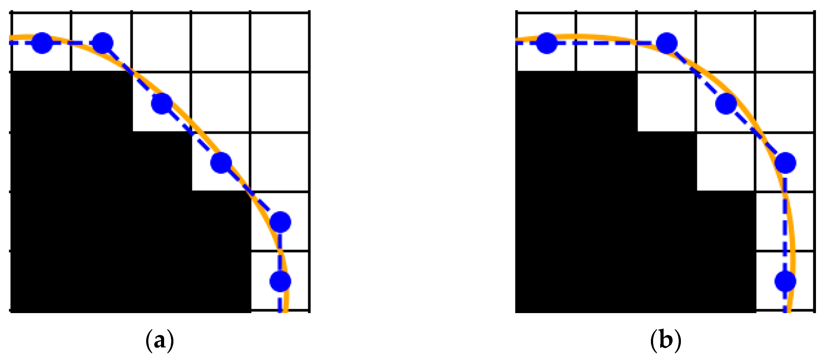
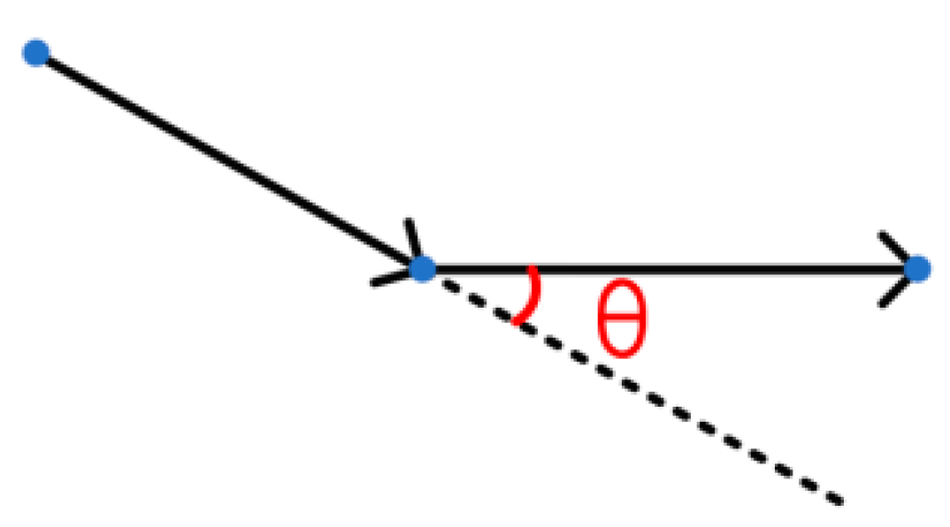
3.2. Control Point Adjustment

The B-spline interpolation method generates a smooth path based on the number and position of control points. However, this method lacks inherent obstacle avoidance capabilities. If control points are not properly selected, the planned path might not stay safely away from obstacles, which could cause collisions [31].

Therefore, the path nodes generated by the SSA-A* cannot be directly used as control points for B-spline smoothing. Instead, these nodes must be adjusted in terms of quantity and position before serving as control points for the B-spline smoothing process. This adjustment ensures that the generated smooth path avoids obstacles effectively.

To achieve appropriate control point adjustment, we propose a two-stage optimization strategy: corner avoidance and path obstacle avoidance.

The corner avoidance strategy adjusts the number and position of control points at path corners based on the spatial relationships of path nodes, enabling the path to navigate turns without colliding with obstacles. First, we define a diagonal judgment function $Diagonal()$ as (10) and two midpoint functions $C()$ and $D()$ as (11).

$$Diagonal\left(A,B\right)=\left|x_A-x_B\right|\wedge \left|y_A-y_B\right|$$

(10)

$$C\left(A,B\right)=\left(x_A,y_B\right) , D\left(A,B\right)=\left(x_B,y_A\right)$$

(11)

Next, we define the path insertion function. For a given path $P=\left(p_1,p_2,\dots ,p_n\right)$, inserting a point $q$ at position $i$ results in the following updated path, as expressed in (12).

$$Insert\left(P,i,q\right)=\left(p_1,\dots ,p_i,q,p_{i+1},\dots ,p_n\right)$$

(12)

Similarly, we define the path deletion function. Given a path $P=\left(p_1,p_2,\dots ,p_n\right)$ and a set of points $R$ to be removed, the updated path after deletion is given by (13).

$$Remove\left(P,R\right)=\{p\in P | p\notin R\vee p\in \left\{p_1,p_n\right\}\}$$

(13)

Finally, the corner avoidance optimization function $Optimize\left(P\right)$ is formulated as (14)–(17).

$$Optimize\left(P\right)=Remove\left(InsertPoints\left(P\right),R\right)$$

(14)

$$InsertPoints\left(P\right)={\displaystyle \bigcup }_{i=1}^{n-1}Insert\left(P,i,q_i\right)$$

(15)

$$q_i=\left\{\begin{array}{c}C\left(p_i,p_{i+1}\right) if C\left(p_i,p_{i+1}\right)\notin O, \\ D\left(p_i,p_{i+1}\right) if D\left(p_i,p_{i+1}\right)\notin O,\\ \varnothing otherwise.\end{array}\right.$$

(16)

$$R=\{p_i,p_{i+1} | Diagonal\left(p_i,p_{i+1}\right)\wedge \left(C\left(p_i,p_{i+1}\right)\in O\vee D\left(p_i,p_{i+1}\right)\in O\right)\}$$

(17)

In (16) and (17), $O$ represents the set of obstacles. The pseudo-code for corner avoidance is presented in Algorithm 2.

Algorithm 2: Corner Avoidance Strategy

Input: Grid map $M$, original path $P$ Output: Optimized path $P^{\prime }$ 1: BEGIN: 2: Initialize $P’ \leftarrow P.copy(), R \leftarrow \varnothing$ 3: $i \leftarrow 0$ 4: while $i<len\left(P^{\prime }\right)-1$ do 5:  $A \leftarrow P^{\prime }\left[i\right], B \leftarrow P^{\prime }\left[i+1\right]$ 6:  $x1, y1 \leftarrow A; x2, y2 \leftarrow B$ 7:  if $\left|x1-x2\right|==1$ and $\left|y1-y2\right|==1$ then // Diagonal move 8:   $C \leftarrow \left(x1, y2\right), D \leftarrow \left(x2, y1\right)$ 9:   $has\_obstacle \leftarrow False$ 10:   if $C \in M.obstacles \vee D \in M.obstacles$ then $has\_obstacle \leftarrow True$ 11:   if $has\_obstacle$ then 12:   $R \leftarrow R \cup \left\{A, B\right\}$ // Mark nodes for removal 13:   if $C \notin M.obstacles$ then 14:    $P^{\prime }.insert\left(i+1, C\right)$ // Insert intermediate point C 15:    $i \leftarrow i+1$ // Skip the new point 16:   else if $D \notin M.obstacles$ then 17:    $P’.insert\left(i+1, D\right)$ // Insert intermediate point D 18:    $i \leftarrow i+1$ 19:   end if 20:    continue // Re-check current index 21:  end if 22:   end if 23:  $i \leftarrow i+1$ 24: end while 25: // Remove marked nodes 26: for $p$ in $P’$ do 27:  if $p \in R$ and $p \notin \left\{P\left[0\left],P\right[-1\right]\right\}$ then 28:   remove $p$ from $P^{\prime }$ 29:  end if 30: end for 31: return $P’$ 32: END

By applying $Optimize\left(P\right)$, the adjustment of control points enables obstacle avoidance during turning processes. This optimization ensures that the generated path smoothly navigates around obstacles rather than intersecting them. The effectiveness of this method is illustrated in Figure 3.

Path obstacle avoidance refers to the process of fine-tuning the positions of all control points based on nearby obstacles to ensure the entire path avoids obstacles effectively.

To achieve obstacle avoidance throughout the path, we adjust the positions of control points according to their proximity to obstacles. Therefore, we introduce the distance adjustment function $f\left(d_i\right)$ as (18), which modifies the position of a control point $P\left(x,y\right)$ when there are $N$ nearby obstacles. Given an obstacle $O_i\left(x_i,y_i\right)$ located at a distance $d_i$, the adjusted position of the control point is denoted as $D_i$ and expressed in (19) and (20).

$$f\left(d_i\right)=\left\{\begin{array}{c}{\displaystyle \frac{1}{a+b{e}^{d_i}}}-c d_i<d_0\\ 0 otherwise\end{array}\right.$$

(18)

$${\mathit{u}}_i={\displaystyle \frac{\left(x-x_i , y-y_i\right)}{d_i}}$$

(19)

$${\mathit{D}}_i={\displaystyle \frac{1}{N}}·f\left(d_i\right)·{\mathit{u}}_i$$

(20)

The pseudo-code for path obstacle avoidance is presented in Algorithm 3.

Algorithm 3: Path Obstacle Avoidance with Grid Map

Input: Optimized path $P^{\prime }$; Grid map $M$; Distance threshold $d_0$; Parameters $a, b, c$ Output: Final control point path $P^{″}$ 1: BEGIN: 2: Initialize $P^{″}$ as empty list 3: for $p$ in $P^{\prime }$ do 4:  if $p==P^{\prime }\left[0\right]$ or $p==P^{\prime }\left[-1\right]$ then 5:   append $p$ to $p^{″}$ 6:   continue 7:   end if 8:  Initialize $D_x \leftarrow 0, D_y \leftarrow 0, N \leftarrow 0$ 9: for each obstacle $O_i\left(x_i, y_i\right)$ in $M.obstacles$ do 10:  $d_i \leftarrow sqrt\left({\left(x-x_i\right)}^2+{\left(y-y_i\right)}^2\right)$ 11:  if $d_i<d_0$ then 12:   $f\left(d_i\right) \leftarrow 1/\left(a+b \ast e^x\right)-c$ 13:   $D_x \leftarrow D_x+f\left(d_i\right) \ast \left(x-x_i\right)/d_i$ 14:   $D_y \leftarrow D_y+f\left(d_i\right) \ast \left(y-y_i\right)/d_i$ 15:   $N \leftarrow N+1$ 16:  end if 17: end for 18: if $N>0$ then 19:  $P_{\mathrm{adjusted}} x\leftarrow x+D_x/N$ 20:  $P_{\mathrm{adjusted}} y\leftarrow y+D_y/N$ 21: else 22:  $P_{\mathrm{adjusted}} \leftarrow P$ 23: end if 24: append $P_{\mathrm{adjusted}}$ to $P^{″}$ 25: end for 26: return $P^{″}$ 27: END

By applying path obstacle avoidance to adjust control points, the B-spline smoothed path is optimized to ensure a safe distance from obstacles, enhancing the overall path safety.

4. Experimental Simulation

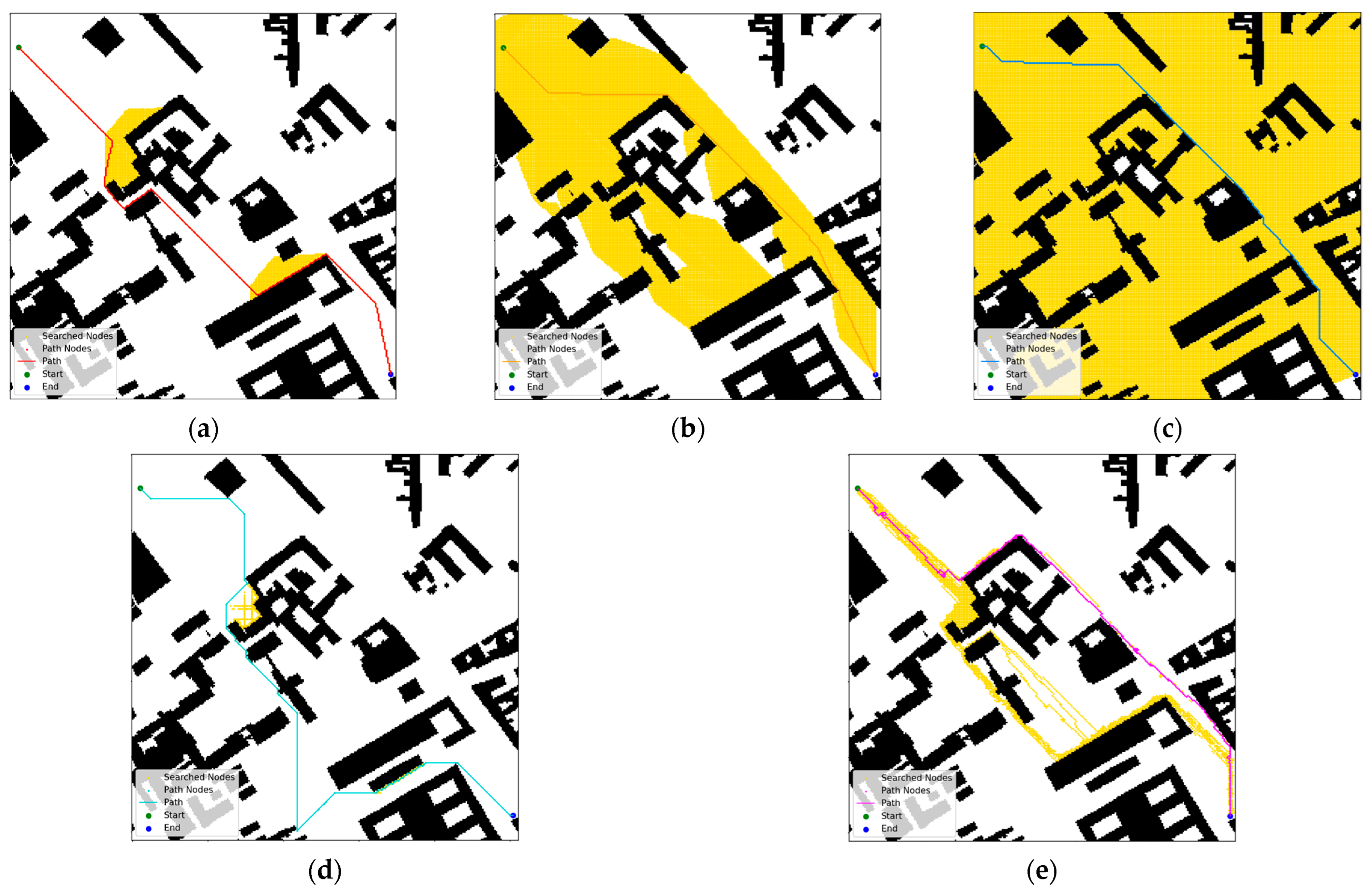
4.1. Path Planning Algorithm Simulation Experiment

4.1.1. Parameters for Path Planning Simulation

We use Python as the development environment. The simulation experiments are conducted in two types of map environments: high-density clustered maps and low-density random maps. Each environment is tested on maps of three different sizes: 20 × 20, 35 × 35, and 50 × 50.

For a given environment and map size, we first apply the SSA-A* to optimize the weight parameters and obtain the heuristic function $h\left(n\right)$. Then, we conduct path planning tests on 15 maps of the same environment and size. The paths generated by the SSA-A* are compared to those produced by Dijkstra’s Algorithm, the Classical A* Algorithm, the JPS-A* Algorithm (an improved version of A* algorithm), and ACO.

The parameters used in the SSA optimization process are listed in

Table 1. Parameters for path planning simulation experiments.

Parameter Name	Value or Range
${\omega }_1$	[0.5, 2]
${\omega }_2$	[0.5, 2]
${\omega }_3$	[0.1, 1]
Population Size $\left(\mathrm{n}\right)$	10
Number of Iterations	100

.

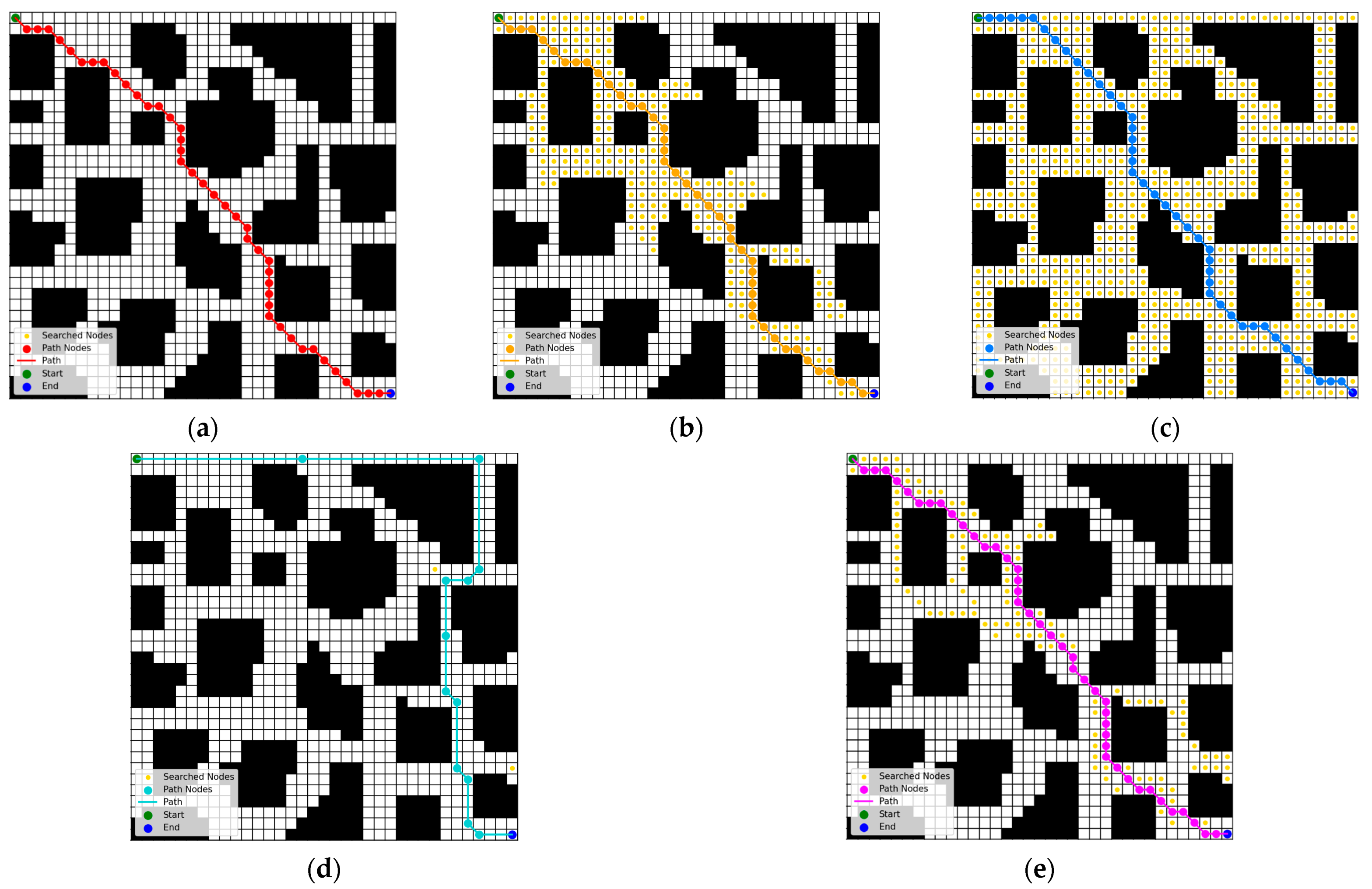
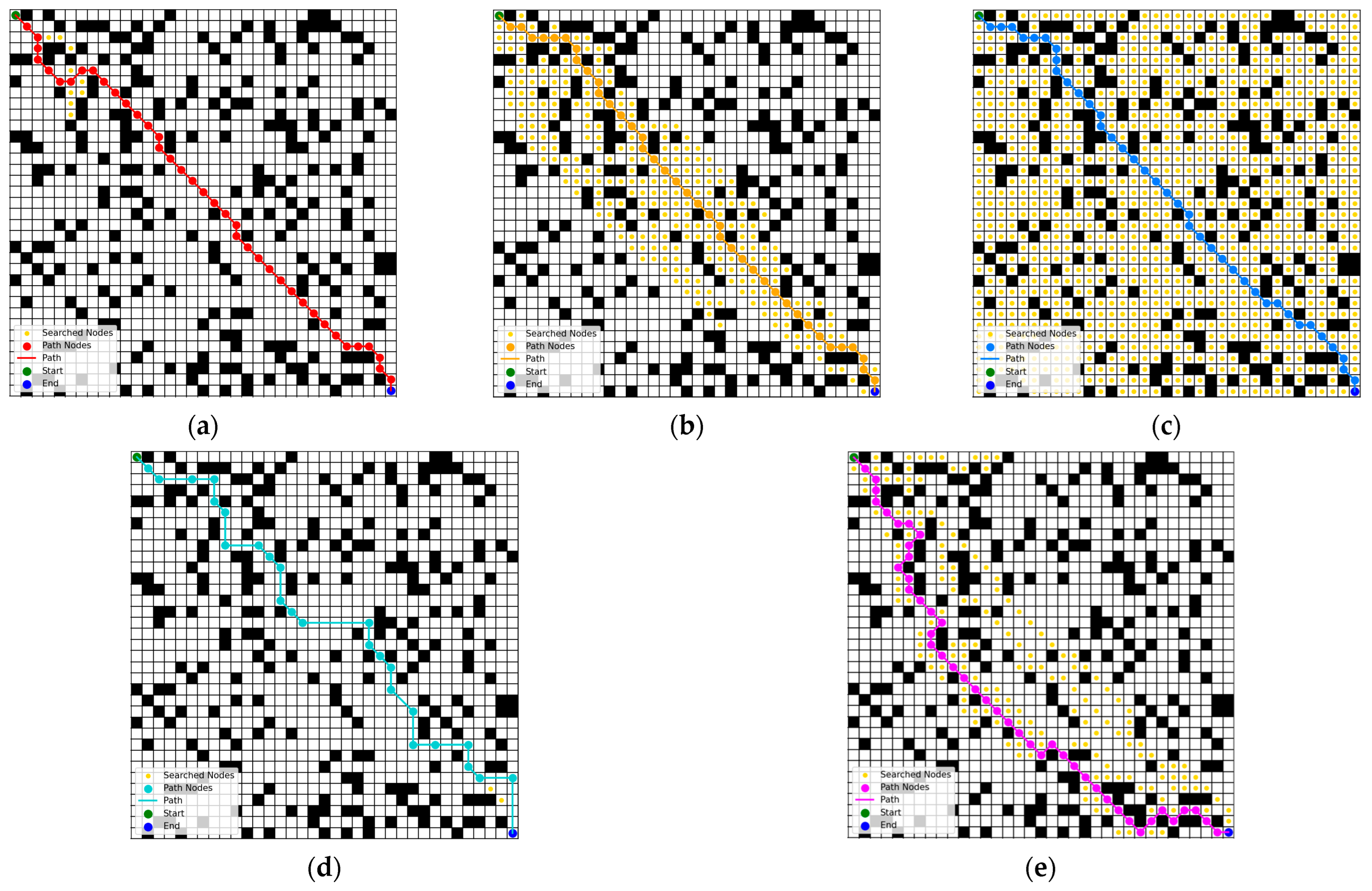
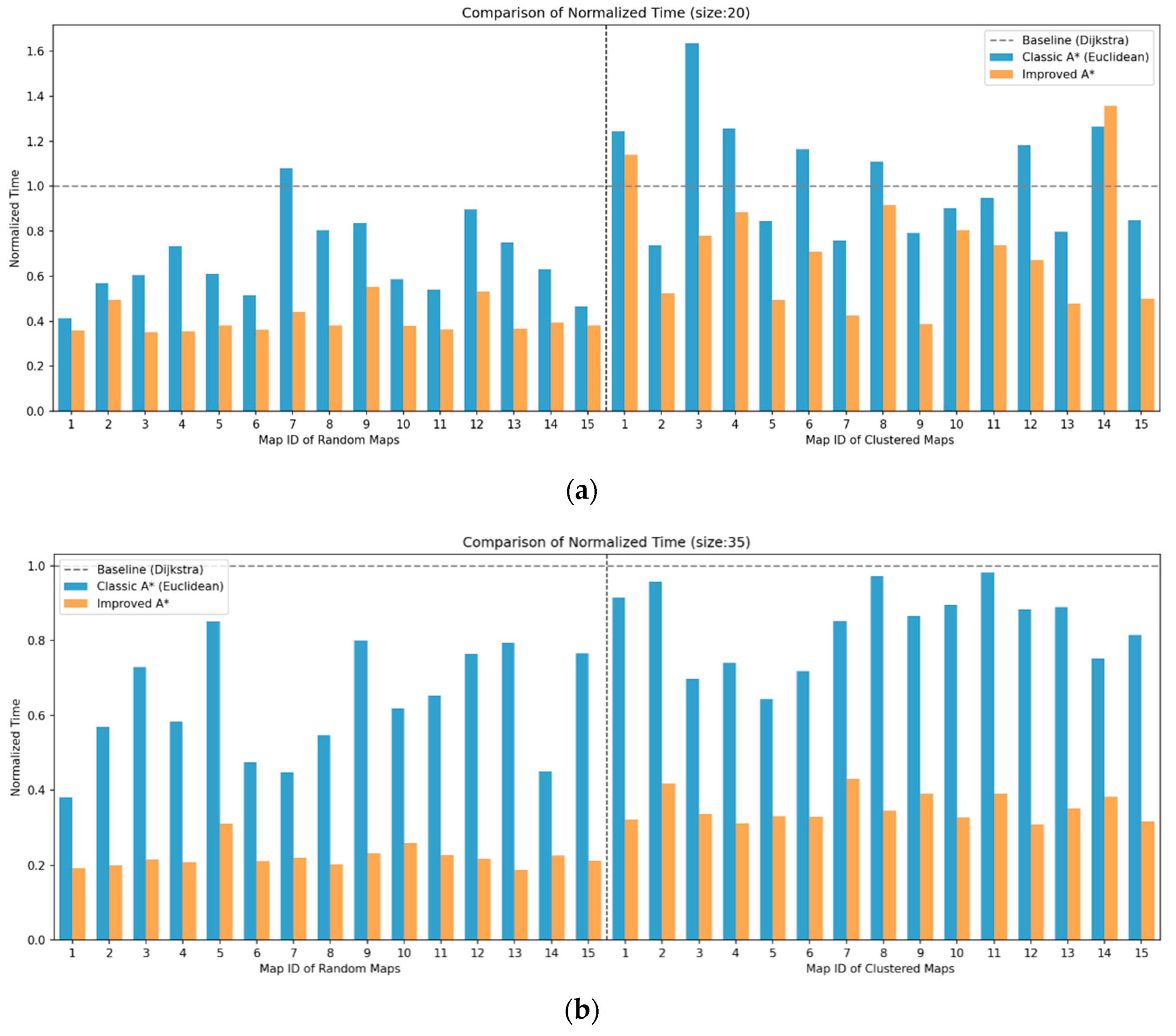
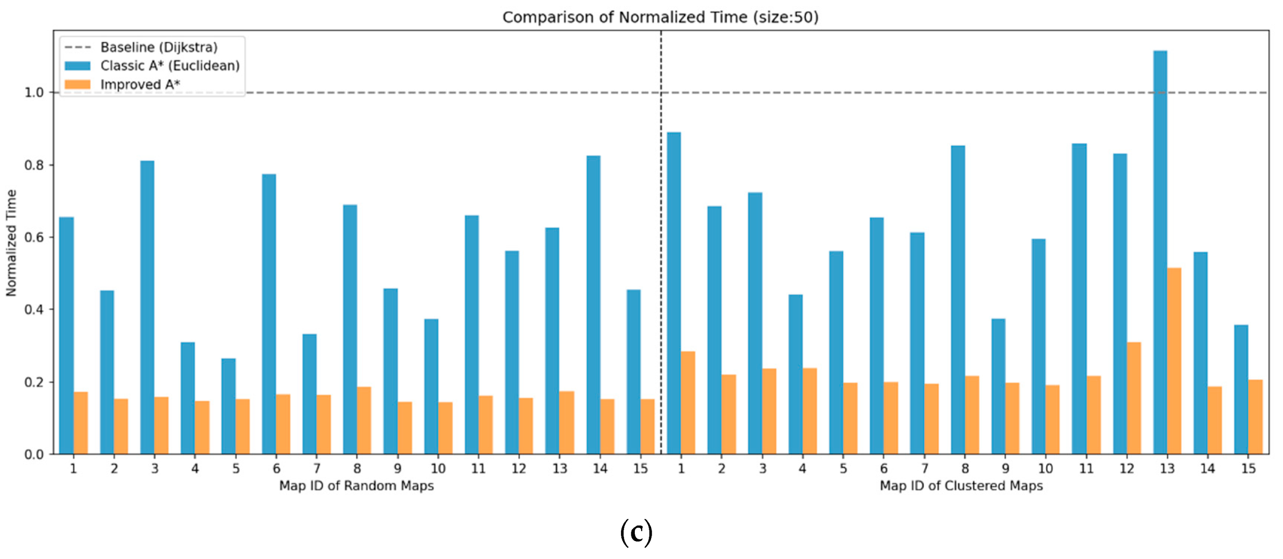
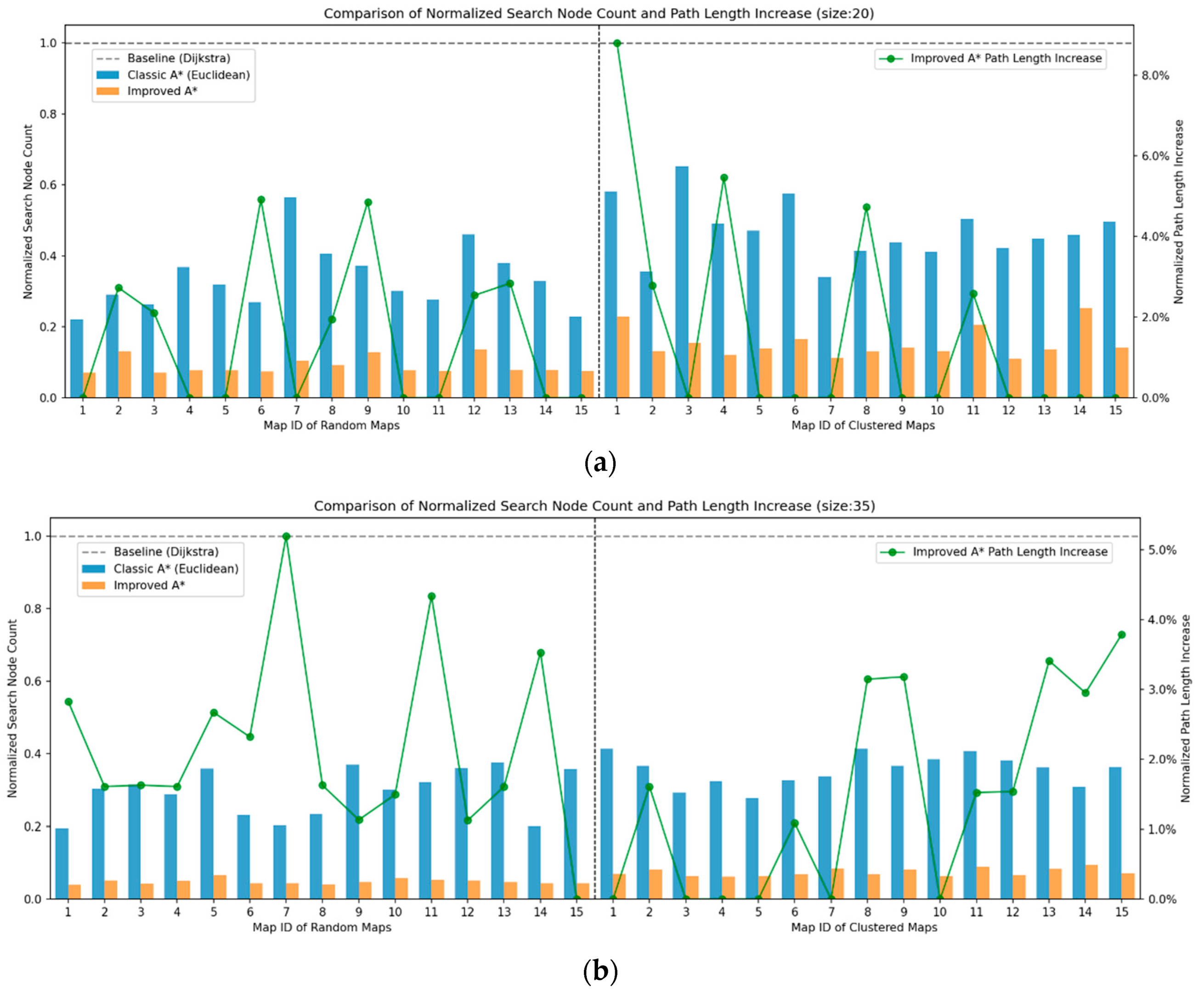
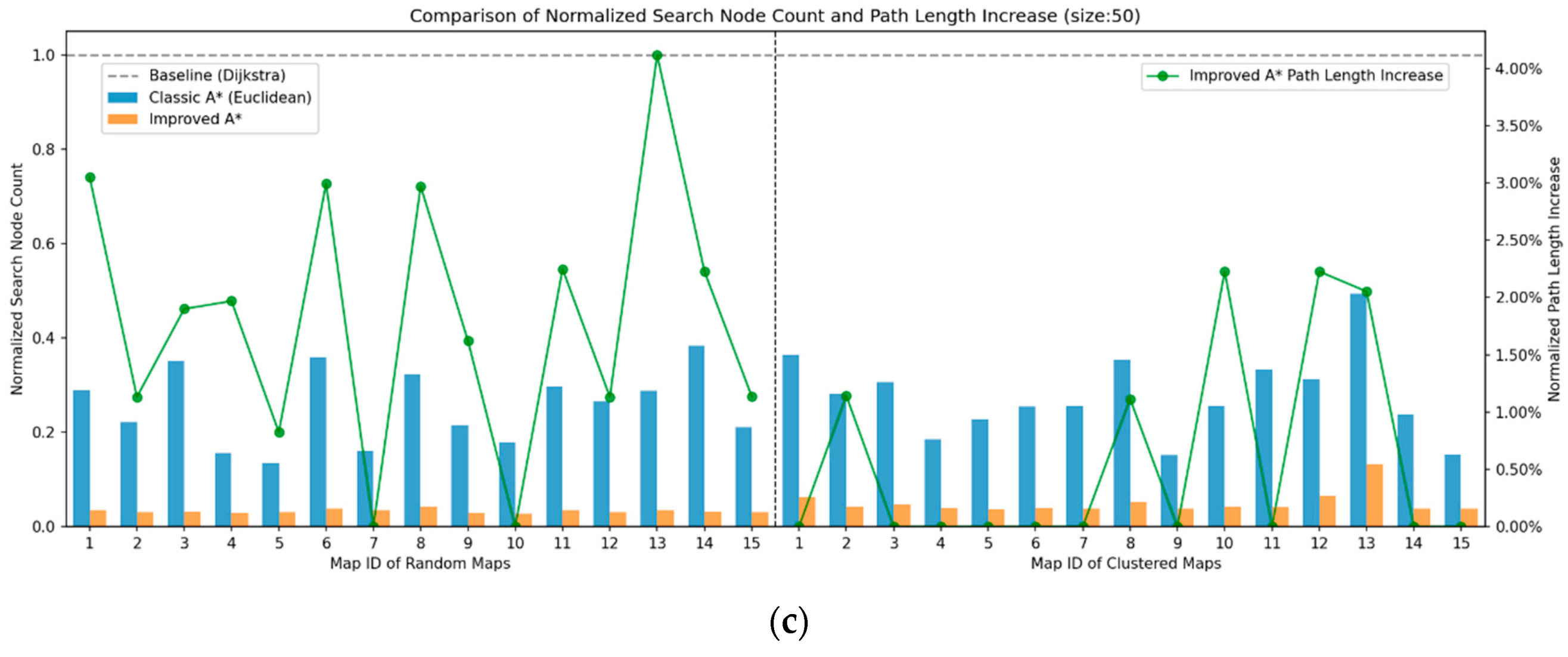
4.1.2. Results and Analysis of Path Planning Simulation Experiment

Figure 4 shows the path planning simulation experimental results for a high-density clustered map on a 35 × 35 grid map. (a) corresponds to the path generated by the SSA-A*. (b) corresponds to the path generated by the Classical A* Algorithm. (c) corresponds to the path generated by Dijkstra’s Algorithm. (d) corresponds to the path generated by the JPS-A* Algorithm. (e) corresponds to the path generated by ACO.

Figure 5 presents the path planning simulation experimental results for a low-density random map on a 35 × 35 grid map. (a) corresponds to the path generated by the SSA-A*. (b) corresponds to the path generated by the Classical A* Algorithm. (c) corresponds to the path generated by Dijkstra’s Algorithm. (d) corresponds to the path generated by the JPS-A* Algorithm. (e) corresponds to the path generated by ACO.

Table 2. Path planning data for a 35 × 35 grid map.

Map ID	Algorithm	Cluster Maps			Random Maps
		SN	Length	Time (ms)	SN	Length	Time (ms)
1	SSA-A*	44	53.36	1.41	39	51.25	0.78
	A*	261	53.36	4.01	191	49.84	1.54
	Dijkstra	631	53.36	4.38	979	49.84	4.05
	JPS-A*	16	71.66	1.01	30	62.14	0.62
	ACO	235	54.18	24.15	234	50.43	26.55
2	SSA-A*	53	52.43	1.82	50	52.43	0.92
	A*	239	51.6	4.17	297	51.60	2.64
	Dijkstra	651	51.6	4.35	982	51.60	4.63
	JPS-A*	23	62.38	1.51	29	60.97	0.9
	ACO	248	51.6	31.31	190	54.43	23.33
3	SSA-A*	41	51.6	1.38	41	51.84	0.99
	A*	187	51.6	2.86	309	51.01	3.34
	Dijkstra	641	51.6	4.1	981	51.01	4.58
	JPS-A*	26	58.63	1.47	27	62.14	0.85
	ACO	191	52.43	28.24	206	53.25	24.77
4	SSA-A*	40	51.01	1.42	48	52.43	0.97
	A*	209	51.01	3.37	278	51.60	2.72
	Dijkstra	644	51.01	4.55	967	51.60	4.66
	JPS-A*	21	66.63	1.45	30	61.56	0.79
	ACO	233	51.6	31.85	235	55.50	25.22
5	SSA-A*	41	51.01	1.41	55	53.60	1.19
	A*	178	51.01	2.75	338	52.77	3.25
	Dijkstra	643	51.01	4.27	940	52.77	3.82
	JPS-A*	36	61.8	2.38	37	61.80	0.69
	ACO	205	52.43	31.69	137	58.08	12.26
6	SSA-A*	45	53.94	1.47	43	51.60	0.84
	A*	214	53.36	3.21	229	50.43	1.89
	Dijkstra	654	53.36	4.47	989	50.43	3.98
	JPS-A*	21	59.21	1.52	25	61.56	0.66
	ACO	295	54.77	33.05	170	50.43	29.83
7	SSA-A*	52	51.01	1.77	43	52.43	0.86
	A*	207	51.01	3.51	201	49.84	1.75
	Dijkstra	612	51.01	4.12	993	49.84	3.91
	JPS-A*	20	70.38	1.58	30	62.97	0.77
	ACO	251	51.84	24.81	168	51.25	29.35
8	SSA-A*	43	54.43	1.54	40	51.25	0.81
	A*	260	52.77	4.34	230	50.43	2.19
	Dijkstra	629	52.77	4.46	983	50.43	4
	JPS-A*	19	63.31	1.45	24	62.73	0.64
	ACO	242	56.43	34.47	230	61.74	24.88
9	SSA-A*	52	53.84	1.72	46	52.77	0.88
	A*	234	52.18	3.8	364	52.18	3.04
	Dijkstra	639	52.18	4.39	983	52.18	3.8
	JPS-A*	15	58.63	1.05	26	62.14	0.69
	ACO	292	60.08	36.16	202	57.84	28.28
10	SSA-A*	42	52.18	1.45	58	56.43	0.99
	A*	251	52.18	3.96	300	55.60	2.37
	Dijkstra	653	52.18	4.42	995	55.60	3.83
	JPS-A*	17	62.73	1.38	89	80.63	2.26
	ACO	220	52.18	31.52	273	60.67	29.63
11	SSA-A*	52	55.36	1.53	53	53.84	0.89
	A*	239	54.53	3.84	319	51.60	2.55
	Dijkstra	586	54.53	3.91	994	51.60	3.9
	JPS-A*	19	60.04	1.29	35	60.63	0.88
	ACO	177	56.18	35.74	233	53.84	25.41
12	SSA-A*	44	54.18	1.41	51	52.18	0.85
	A*	251	53.36	4.02	353	51.60	2.99
	Dijkstra	657	53.36	4.55	977	51.60	3.91
	JPS-A*	17	69.21	1.38	43	63.56	1.23
	ACO	192	55.01	36.54	242	54.18	24.47
13	SSA-A*	52	53.36	1.47	45	52.43	0.83
	A*	227	51.6	3.72	362	51.60	3.51
	Dijkstra	627	51.6	4.18	965	51.60	4.42
	JPS-A*	23	67.31	1.49	30	62.14	0.83
	ACO	169	53.84	33.62	239	54.67	26.32
14	SSA-A*	57	57.94	1.67	43	51.60	1.03
	A*	188	56.28	3.28	194	49.84	2.05
	Dijkstra	609	56.28	4.36	971	49.84	4.55
	JPS-A*	19	62.63	2.5	25	58.63	0.74
	ACO	171	58.77	36.19	187	52.08	26.83
15	SSA-A*	45	54.77	1.5	43	51.60	0.98
	A*	229	52.77	3.86	346	51.60	3.53
	Dijkstra	630	52.77	4.73	968	51.60	4.61
	JPS-A*	20	68.63	2	26	60.97	0.74
	ACO	189	57.6	32.46	251	52.43	25.72

shows the detailed data of path planning on a 35 × 35 grid map for both high-density clustered maps and low-density random maps. In this table, SN represents the number of search nodes.

Figure 6 shows the comparison of the running time between the SSA-A* and the Classical A* Algorithm. The running times of both algorithms are normalized with respect to the running time of Dijkstra’s Algorithm (Dijkstra = 1). A lower value indicates a shorter running time.

Figure 7 presents a comparison of the search node count and path length between the SSA-A* and Classical A* Algorithms. Search Efficiency (Left Axis): The number of search nodes for both the SSA-A* and Classical A* algorithms is normalized with respect to the number of search nodes in Dijkstra’s Algorithm (Dijkstra = 1). A lower value indicates higher search efficiency. Path Quality (Right Axis): The SSA-A* path length increase (relative to the shortest path from Dijkstra) is shown as a percentage.

Table 3. Comparison of the average performance of the SSA-A* and other algorithms.

Map Size		20		35		50
Map Type		Cluster Map	Random Map	Cluster Map	Random Map	Cluster Map	Random Map
Average Time Reduction in SSA-A*	vs. A* (%)	30.79%	36.56%	57.45%	63.09%	62.82%	67.75%
	vs. Dijkstra (%)	27.89%	59.35%	64.69%	77.85%	75.94%	84.12%
	vs. ACO (%)	95.57%	96.92%	95.16%	96.16%	95.04%	97.61%
Average Searched Nodes Reduction in SSA-A*	vs. A* (%)	67.17%	72.52%	78.87%	83.08%	81.86%	86.10%
	vs. Dijkstra (%)	84.64%	91.01%	92.58%	95.19%	95.00%	96.73%
	vs. ACO (%)	64.32%	71.83%	78.03%	77.43%	79.37%	82.75%
Average Distance Increase in SSA-A* vs. A* (%)		1.62%	1.46%	1.48%	2.18%	0.58%	1.82%
Average Distance Reduction in SSA-A*	vs. JPS-A* (%)	14.85%	18.93%	22.24%	22.33%	15.00%	21.96%
	vs. ACO (%)	4.45%	4.72%	2.17%	3.76%	5.41%	5.00%

presents a comparison of the average performance of the SSA-A* against other algorithms across different map sizes.

Based on the simulation experimental results, for the high-density clustered map, the SSA-A* reduces the running time by an average of 56.17% compared to Dijkstra’s Algorithm, by 50.35% compared to the A* algorithm, and by 95.26% compared to ACO. The SSA-A* reduces the number of search nodes by an average of 91.41% compared to Dijkstra’s Algorithm, by 75.97% compared to the A* algorithm, and by 73.91% compared to ACO.

For the low-density random map, the SSA-A* reduces the running time by an average of 73.77% compared to Dijkstra’s Algorithm, by 55.80% compared to the A* algorithm, and by 96.90% compared to ACO. The SSA-A* reduces the number of search nodes by an average of 94.31% compared to Dijkstra’s Algorithm, by 80.57% compared to the A* Algorithm, and by 77.34% compared to ACO.

With the increase in map size, the advantages of the SSA-A* become more apparent. For example, on the 50 × 50 low-density random map, the SSA-A* reduces the running time by 67.75% compared to Dijkstra’s Algorithm and by 84.12% compared to the A* algorithm. Additionally, the number of search nodes is reduced by 96.73% compared to Dijkstra’s Algorithm and by 86.10% compared to the A* algorithm. In all cases, the JPS-A* algorithm shows an average increase in path length of 14% or more compared to the shortest path, while ACO shows an increase of 4.25%. In contrast, the SSA-A* increases the path length by only 0.5% to 2.2%, enhancing its suitability for practical applications.

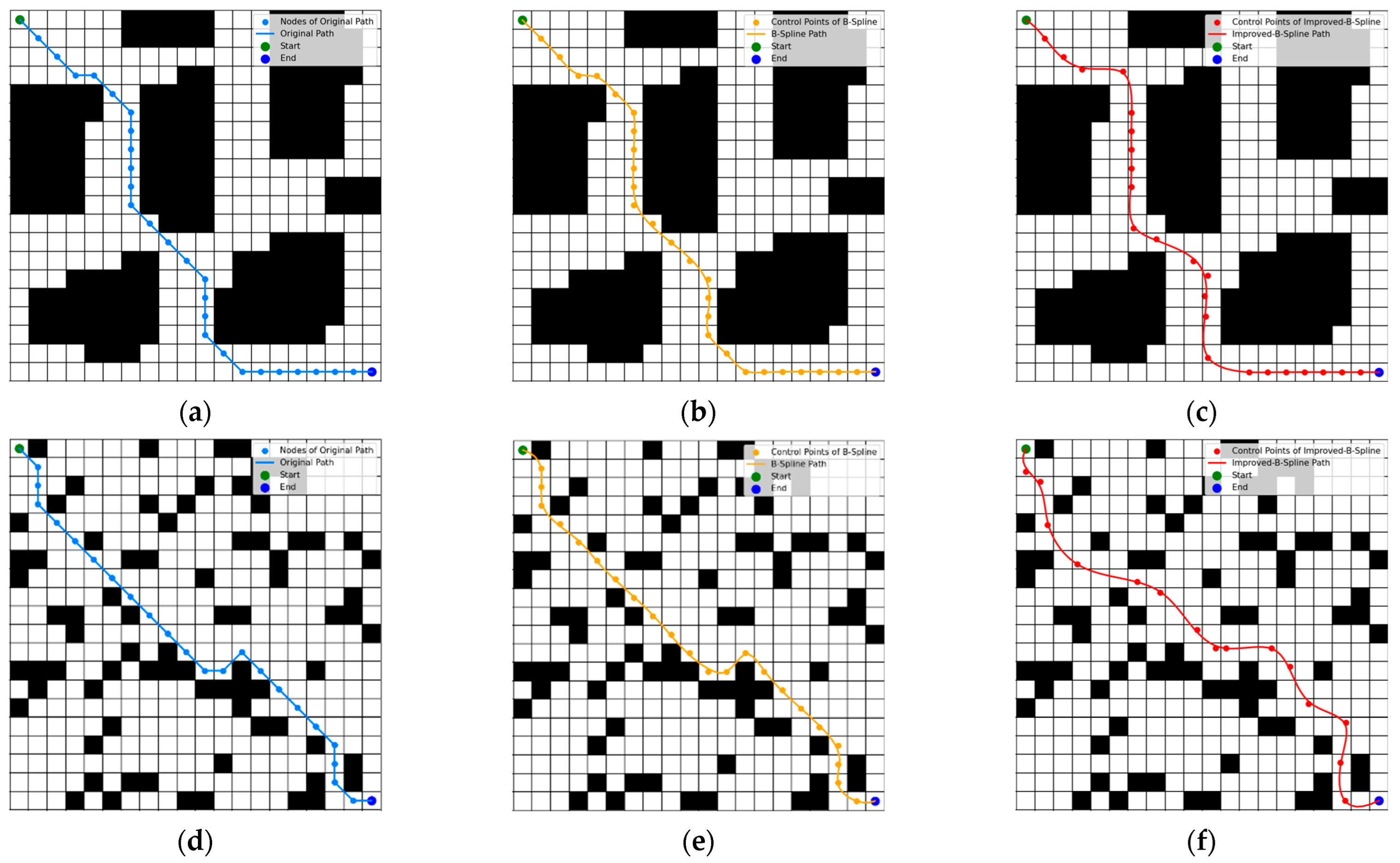
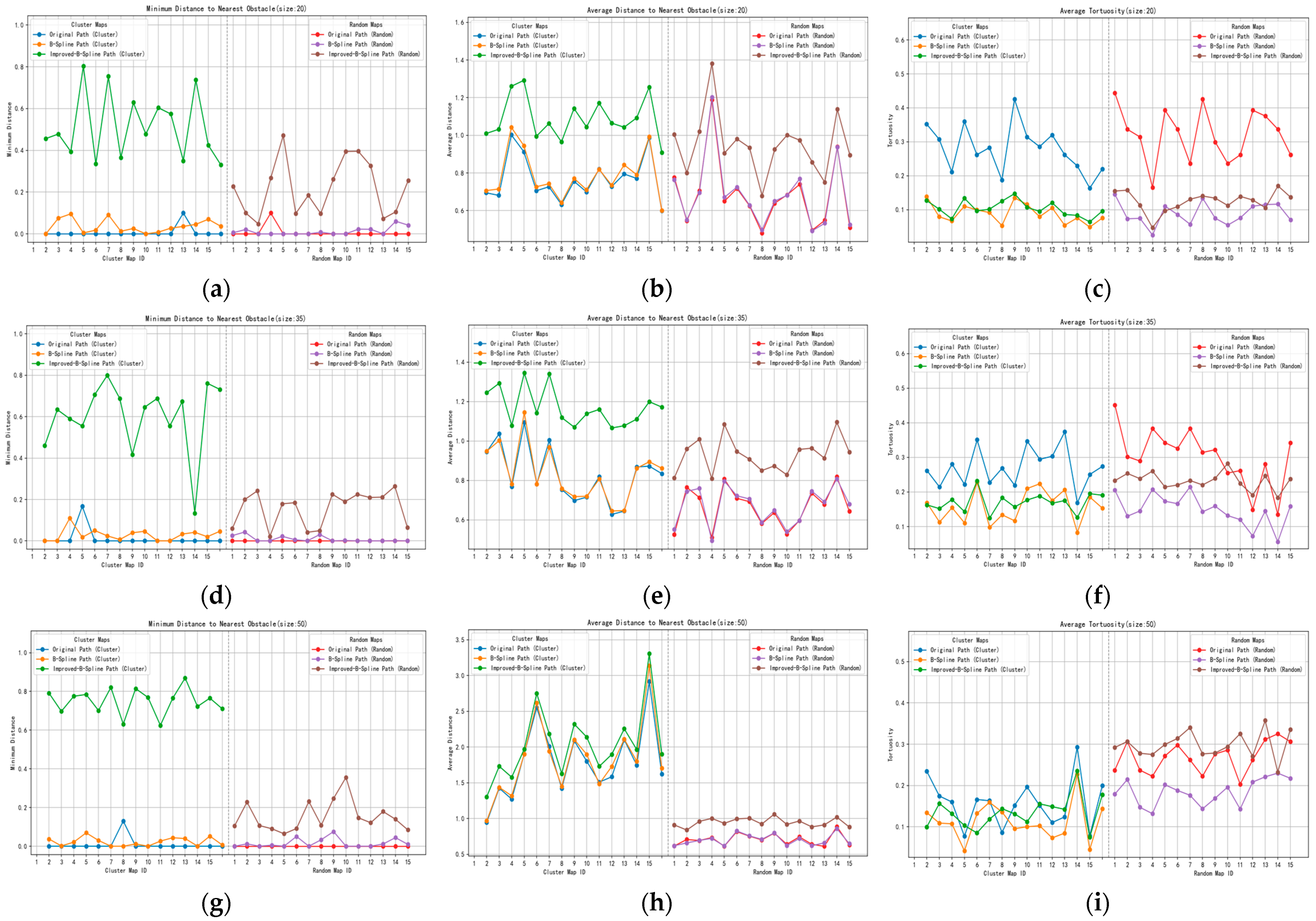
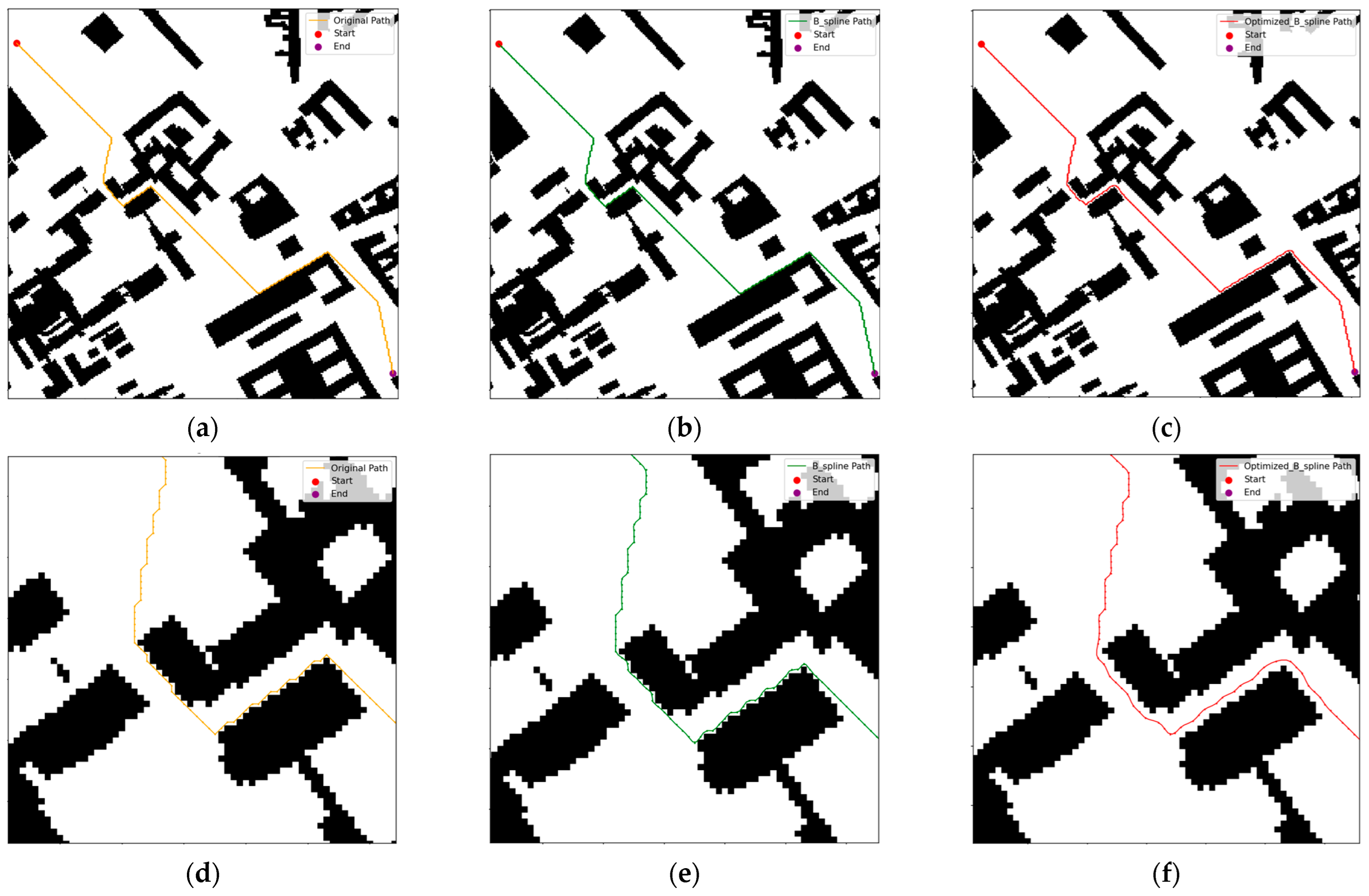
4.2. Path Smoothing Algorithm Simulation Experiment

4.2.1. Parameters for the Path Smoothing Algorithm Simulation Experiment

Python was used as the development environment, and grid maps of sizes 20 × 20, 35 × 35, and 50 × 50 were selected. The obstacle density and distribution methods were set to high-density clustering and low-density random, respectively, to represent the entire environmental information. The maps were categorized into six groups according to the above standards, with each group consisting of 15 different maps for testing. In the maps, the green circle represents the start point, the blue circle represents the endpoint, the light blue line represents the initial path, the orange line represents the path after smoothing with the B-spline algorithm, and the red line represents the path after smoothing with the improved B-spline algorithm.

The parameters for the B-spline algorithm used in the simulation experiment are shown in

Table 4. Parameter settings of B-spline interpolation.

Parameter Name	Parameter Value
Smoothing Factor ($s$)	0.1
Number of Interpolation Points	100

.

In B-spline interpolation, the smoothing factor is used to control the smoothness of the B-spline curve, while the number of interpolation points determines the accuracy and computational complexity of the B-spline curve. After repeated experiments, the smoothing factor was set to 0.1, and the number of interpolation points was set to 100.

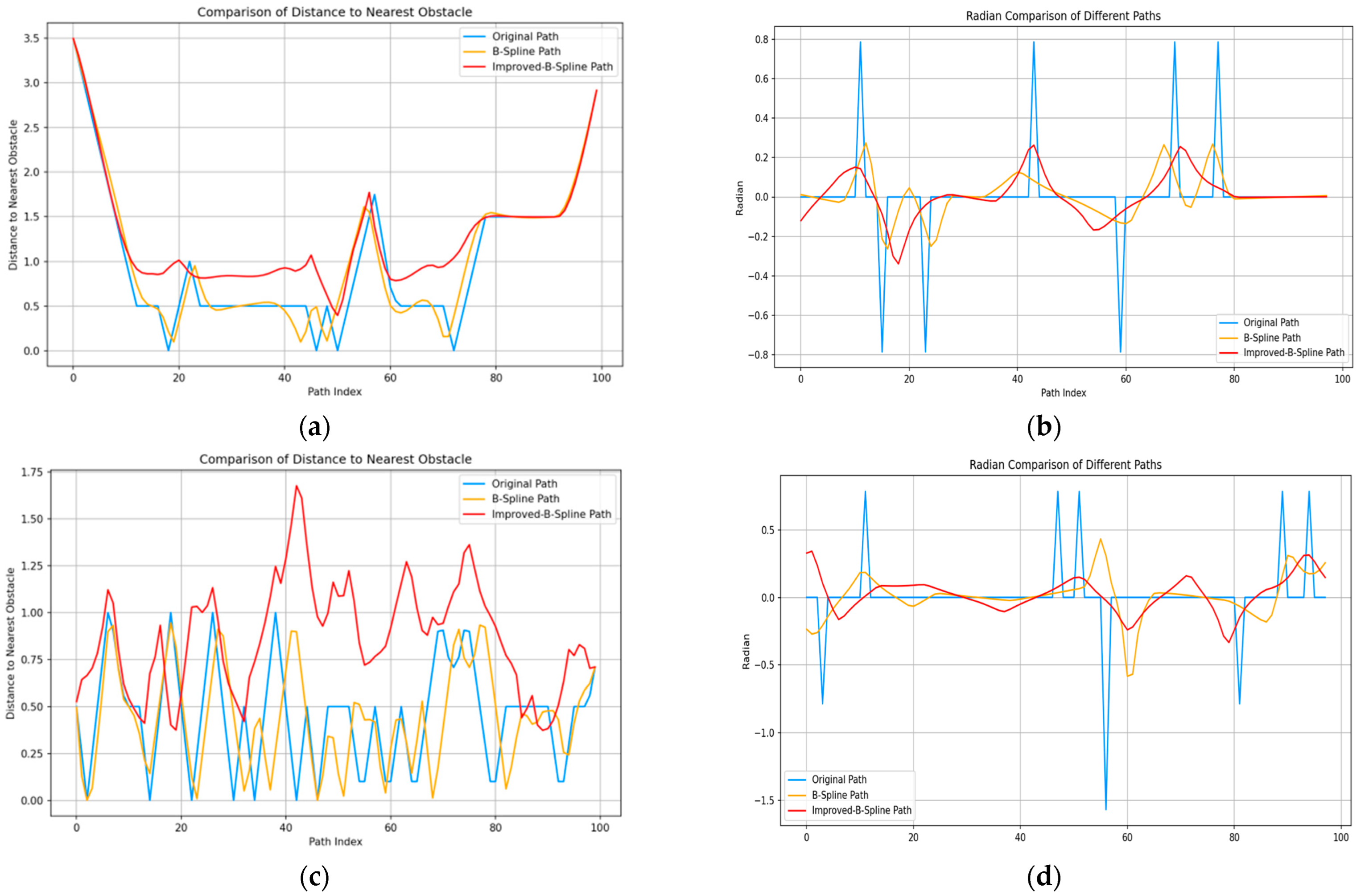
4.2.2. Results and Analysis of the Path Smoothing Algorithm Simulation Experiment

Based on the aforementioned simulation environment and parameter settings, simulation experiments were conducted to calculate the smoothed paths for different algorithms. The results are presented for a high-density clustered map of size 20 × 20 (in the upper part of Figure 8) and a low-density random map (in the bottom part of Figure 8). As shown in (a) and (e), the original path contains multiple dangerous points near obstacles, with the distance between the path and obstacles being too small, which could lead to collisions. In (b) and (f), after B-spline interpolation smoothing, the path becomes noticeably smoother and more continuous, with no sharp corners; however, the path still remains too close to the obstacles. As shown in (c) and (g), after smoothing with the improved B-spline algorithm, the path not only maintains a safe distance from the obstacles but also remains continuous and smooth.

The performance of the original path, the path smoothed by the B-spline algorithm, and the path smoothed by the improved B-spline algorithm is evaluated below. The evaluation primarily focuses on two key metrics: the curvature of the path and the distance from the path to the nearest obstacle.

The logic for calculating the degree of meandering is as follows: As shown in Figure 9, adjacent points in the path are connected to form two vectors. The angle between these vectors is calculated, and the rate of change in this angle is determined. This rate of change is defined as the degree of meandering. A smaller degree of meandering indicates a smoother path.

The distance from the path to the obstacle is one of the important indicators for measuring the safety of the path. The greater the distance from the path to the obstacle, the higher the safety and reliability of the path. Here, the distance from each point on the path to the nearest obstacle is calculated to assess the safety of the path.

In Figure 10, (a) and (b) compare the curvature of the paths and the distance from the paths to the nearest obstacle for each algorithm on the clustered map displayed above. (c) and (d) compare the curvature of the paths and the distance of the paths to the nearest obstacle for each algorithm on the random map displayed above. As can be seen from the figures, after smoothing with the improved B-spline algorithm, the path maintains the largest distance from the nearest obstacle, with a moderate curvature, thereby meeting the requirements.

Table 5. Performance comparison of each path.

Map ID	Algorithm	Cluster Maps			Random Maps
		MD	AD	AT	MD	AD	AT
1	A	0.0000	0.6945	0.3521	0.0000	0.7765	0.4439
	B	0.0000	0.7063	0.1387	0.0060	0.7638	0.1452
	C	0.4564	1.0097	0.1270	0.2277	1.0051	0.1549
2	A	0.0000	0.6809	0.3073	0.0000	0.5451	0.3366
	B	0.0752	0.7149	0.0792	0.0213	0.5507	0.0732
	C	0.4781	1.0321	0.1014	0.1000	0.7996	0.1575
3	A	0.0000	1.0024	0.2115	0.0000	0.7057	0.3142
	B	0.0961	1.0423	0.0668	0.0000	0.6960	0.0746
	C	0.3939	1.2601	0.0730	0.0480	1.0206	0.1132
4	A	0.0000	0.9127	0.3600	0.1000	1.1887	0.1653
	B	0.0046	0.9452	0.1102	0.0000	1.2021	0.0252
	C	0.8040	1.2919	0.1340	0.2677	1.3819	0.0469
5	A	0.0000	0.7055	0.2618	0.0000	0.6499	0.3927
	B	0.0183	0.7269	0.0994	0.0000	0.6707	0.1102
	C	0.3346	0.9950	0.0964	0.4718	0.9050	0.0967
6	A	0.0000	0.7267	0.2827	0.0000	0.7176	0.3366
	B	0.0919	0.7426	0.0915	0.0000	0.7250	0.0857
	C	0.7542	1.0624	0.1014	0.0975	0.9804	0.1088
7	A	0.0000	0.6324	0.1870	0.0000	0.6256	0.2356
	B	0.0127	0.6415	0.0532	0.0000	0.6289	0.0569
	C	0.3643	0.9650	0.1250	0.1845	0.9347	0.1308
8	A	0.0000	0.7558	0.4254	0.0000	0.4808	0.4254
	B	0.0260	0.7715	0.1350	0.0084	0.4984	0.1336
	C	0.6290	1.1425	0.1471	0.0974	0.6789	0.1402
9	A	0.0000	0.6990	0.3142	0.0000	0.6392	0.2992
	B	0.0000	0.7113	0.1155	0.0000	0.6500	0.0748
	C	0.4775	1.0443	0.1069	0.2611	0.9248	0.1339
10	A	0.0000	0.8205	0.2856	0.0000	0.6837	0.2356
	B	0.0084	0.8199	0.0793	0.0000	0.6818	0.0546
	C	0.6038	1.1713	0.0950	0.3946	1.0015	0.1122
11	A	0.0000	0.7276	0.3200	0.0000	0.7396	0.2618
	B	0.0277	0.7350	0.1053	0.0227	0.7692	0.0760
	C	0.5741	1.0648	0.1206	0.3956	0.9740	0.1391
12	A	0.1000	0.7944	0.2618	0.0000	0.4960	0.3927
	B	0.0359	0.8430	0.0541	0.0221	0.4932	0.1104
	C	0.3501	1.0428	0.0859	0.3259	0.8577	0.1283
13	A	0.0000	0.7710	0.2291	0.0000	0.5484	0.3756
	B	0.0458	0.7907	0.0758	0.0000	0.5329	0.1150
	C	0.7377	1.0929	0.0833	0.0731	0.7502	0.1057
14	A	0.0000	0.9868	0.1636	0.0000	0.9388	0.3366
	B	0.0702	0.9931	0.0487	0.0606	0.9384	0.1163
	C	0.4245	1.2563	0.0641	0.1057	1.1389	0.1701
15	A	0.0000	0.5984	0.2199	0.0000	0.5090	0.2618
	B	0.0365	0.6015	0.0754	0.0419	0.5247	0.0702
	C	0.3309	0.9086	0.0961	0.2562	0.8942	0.1368

compares the minimum distance (MD) to the nearest obstacle, the average distance (AD) to the nearest obstacle, and the average curvature (AT) of the initial path (A), the path smoothed by the B-spline algorithm (B), and the path smoothed by the improved B-spline algorithm (C) for two types of maps with a size of 20 × 20.

The following conclusions can be drawn:

In the high-density clustered map, the average minimum distance from the smoothed path of the improved B-spline algorithm to the nearest obstacle increased by 0.5142 compared to the initial path and by 0.4776 compared to the B-spline algorithm’s smoothed path. The average distance from the improved B-spline algorithm smoothed path to the nearest obstacle increased by 43.05% compared to the initial path and by 39.82% compared to the B-spline algorithm smoothed path. The average curvature of the improved algorithm smoothed path decreased by 61.87% compared to the initial path.

In the low-density random map, the average minimum distance from the improved B-spline algorithm’s smoothed path to the nearest obstacle increased by 0.2137 compared to the initial path and by 0.2082 compared to the B-spline algorithm’s smoothed path. The average distance from the improved B-spline algorithm’s smoothed path to the nearest obstacle increased by 42.20% compared to the initial path and by 41.04% compared to the B-spline algorithm’s smoothed path. The average curvature of the improved algorithm’s smoothed path decreased by 59.96% compared to the initial path.

Figure 11 shows the performance comparison of all maps in the test set, categorized by size. It presents line graphs of the minimum distance to the nearest obstacle, the average distance to the nearest obstacle, and the average curvature for two types of maps with a size of 20 × 20. The same classification and visualization are applied to the other two map sizes. From the figure, it is clearly observed that the distance from the path smoothed by the improved B-spline algorithm to the nearest obstacle is always the largest, the average distance to the nearest obstacle is also the largest, and the average curvature is moderate, significantly reduced compared to the original path.

4.3. Benchmark Tests

The tests were conducted using the city/street maps dataset from the MovingAI 2D Pathfinding Benchmarks, running on hardware with a Ryzen 7 6800H/RTX 3060 Laptop GPU configuration, with the algorithm implemented in Python 3.12.

Figure 12 presents the results of benchmark tests on a 256 × 256 map. (a) corresponds to the path generated by the SSA-A*. (b) corresponds to the path generated by the Classical A* Algorithm. (c) corresponds to the path generated by Dijkstra’s Algorithm. (d) corresponds to the path generated by the JPS-A* Algorithm. (e) corresponds to the path generated by ACO.

Table 6. Performance comparison of path planning algorithms in benchmark tests.

Algorithm	Comparison to A* (100%)
	Searched-Nodes (%)	Length (%)	Time (%)
SSA-A*	4.39	104.83	6.31
Dijkstra	320.17	100.00	94.08
A*-JPS	0.70	130.75	325.38
ACO	12.04	132.65	210.45

presents the performance comparison results of various path planning algorithms in benchmark tests. The test results demonstrate that the SSA-A* reduces pathfinding time by 93.69% compared to the A* algorithm and by 93.30% compared to Dijkstra’s Algorithm. The paths planned by the SSA-A*, JPS-A* algorithm, and ACO exhibit increases of 4.08%, 30.75%, and 32.65%, respectively, relative to the shortest path, while their average runtime accounts for 6.31%, 352.38%, and 210.45% of the A* algorithm’s runtime. This discrepancy arises because the JPS -A* algorithm incurs redundant computations due to its jump strategy in real-world scenarios with irregular obstacles, leading to inefficiency and longer planned paths. Meanwhile, the ACO tends to select suboptimal branches in early iterations due to randomness, resulting in circuitous paths. In contrast, the SSA-A* demonstrates superior performance in both path length and planning time.

Figure 13 presents the benchmark test results of five path smoothing algorithms on a 256 × 256 map. (a) and (d) show the global view and local details of the original path; (b) and (e) display the globally smoothed path and its local section after B-spline interpolation; (c) and (f) demonstrate the panoramic and zoomed-in views of the path processed by the improved B-spline interpolation smoothing algorithm.

For the path smoothing algorithms, the test results indicate that the Improved B-spline Path increases the minimum distance to the nearest obstacle by 0.78 compared to the Original Path and by 0.77 compared to the B-spline Path. Additionally, the average distance to the nearest obstacle for the Improved B-spline Path increases by 17.40% compared to the Original Path and by 14.93% compared to the B-Spline Path. Furthermore, the average curvature of the Improved B-spline Path decreases by 53.86% compared to the Original Path and by 28.54% compared to the B-spline Path.

5. Conclusions

To address the limitations of the traditional A* algorithm, such as low performance and unsmooth paths in path planning, this paper proposes a scheme that improves the A* algorithm by integrating the SSA for path planning, followed by path smoothing using the improved B-spline interpolation method. Through comparative experiments in various scenarios, including high-density clustered environments and low-density random environments, and multiple grid map scales (ranging from 20 × 20 to 50 × 50), the optimized algorithm demonstrates significant advantages in key indicators such as search efficiency, smoothness, and safety, offering a more efficient and reliable path planning approach for practical application scenarios.

However, the SSA-A* still has certain limitations. While the SSA greatly enhances the optimization of the heuristic function, its performance can vary based on the complexity and specific characteristics of the environment. In environments with dynamic obstacles that change frequently, the algorithm may require more frequent re-optimization to adjust to new conditions. Additionally, the current implementation assumes a static environment, and extending it to handle real-time dynamic obstacle environments or 3D path planning requires further adjustments.

Future research could focus on addressing these limitations. One potential direction is the development of adaptive mechanisms that dynamically adjust the SSA parameters based on real-time environmental changes, thereby improving the algorithm’s robustness in dynamic and real-time scenarios. Another approach could involve exploring hybrid algorithms that integrate the SSA-A* with other advanced techniques, such as reinforcement learning or machine learning models, to further enhance path planning performance. Additionally, expanding the algorithm’s scalability to handle more complex 3D path planning scenarios could be another key area for future development. In conclusion, while the SSA-A* offers a promising solution for path planning, continuous research is essential to overcome its current limitations and expand its applicability to a broader range of real-world environments.

References

1. Hassan, M.U.; Ullah, M.; Iqbal, J. Towards Autonomy in Agriculture: Design and Prototyping of a Robotic Vehicle with Seed Selector. In Proceedings of the 2016 2nd International Conference on Robotics and Artificial Intelligence (ICRAI), Rawalpindi, Pakistan, 1–2 November 2016; pp. 37–44. [Google Scholar] [CrossRef]
2. Liu, L.; Wang, X.; Yang, X.; Liu, H.; Li, J.; Wang, P. Path Planning Techniques for Mobile Robots: Review and Prospect. Expert Syst. Appl. 2023, 227, 120254. [Google Scholar] [CrossRef]
3. Bento, L.M.; Boccardo, D.R.; Machado, R.C.; Miyazawa, F.K.; de Sá, V.G.P.; Szwarcfiter, J.L. Dijkstra graphs. Discret. Appl. Math. 2017, 261, 52–62. [Google Scholar] [CrossRef]
4. Xiang, D.; Lin, H.; Ouyang, J.; Huang, D. Combined Improved A* and Greedy Algorithm for Path Planning of Multi-Objective Mobile Robot. Sci. Rep. 2022, 12, 13273. [Google Scholar] [CrossRef]
5. Zhang, T.; Xu, S.; Gao, Y.; Wang, P.; Schonfeld, P.; Zou, Y.; He, Q. 3D Constrained Hybrid A*: Improved Vehicle Path Planning Algorithm for Cost-Effective Road Alignment Design. Autom. Constr. 2024, 166, 105645. [Google Scholar] [CrossRef]
6. Huang, T.; Fan, K.; Sun, W. Density Gradient-RRT: An Improved Rapidly Exploring Random Tree Algorithm for UAV Path Planning. Expert Syst. Appl. 2024, 252, 124121. [Google Scholar] [CrossRef]
7. Huang, Z.; Chen, H.; Pohovey, J.; Driggs-Campbell, K. Neural Informed RRT*: Learning-based Path Planning with Point Cloud State Representations under Admissible Ellipsoidal Constraints. arXiv 2023, arXiv:2309.14595. [Google Scholar] [CrossRef]
8. Worring, A.; Mayer, B.E.; Hamacher, K. Genetic Algorithm Niching by (Quasi-)infinite Memory. In Proceedings of the Genetic and Evolutionary Computation Conference (GECCO ’21), Lille, France, 10–14 July 2021; pp. 296–304. [Google Scholar] [CrossRef]
9. García, M.; López, N.; Rodríguez, I. A Full Process Algebraic Representation of Ant Colony Optimization. Inf. Sci. 2024, 658, 120025. [Google Scholar] [CrossRef]
10. Wu, C.; Zhu, Z.; Tian, Z.; Zou, C. Generational Exclusion Particle Swarm Optimization with Central Aggregation Mechanism. In Advances in Swarm Intelligence; Tan, Y., Shi, Y., Niu, B., Eds.; Lecture Notes in Computer Science; Springer: Cham, Switzerland, 2022; Volume 13344, p. 15. [Google Scholar] [CrossRef]
11. Li, X.; Wang, L.; An, Y.; Huang, Q.L.; Cui, Y.H.; Hu, H.S. Dynamic Path Planning of Mobile Robots Using Adaptive Dynamic Programming. Expert Syst. Appl. 2024, 235, 121112. [Google Scholar] [CrossRef]
12. Xu, Y.; Li, Q.; Xu, X.; Yang, J.; Chen, Y. Research Progress of Nature-Inspired Metaheuristic Algorithms in Mobile Robot Path Planning. Electronics 2023, 12, 3263. [Google Scholar] [CrossRef]
13. Johansson, A.; Markdahl, J. Swarm Bug Algorithms for Path Generation in Unknown Environments. In Proceedings of the 2023 62nd IEEE Conference on Decision and Control (CDC), Singapore, 13–15 December 2023; pp. 6958–6965. [Google Scholar]
14. Wang, M.; Xu, J.; Zhang, J.; Cui, Y. An Autonomous Navigation Method for Orchard Rows Based on a Combination of an Improved A* Algorithm and SVR. Precis. Agric. 2024, 25, 429–453. [Google Scholar] [CrossRef]
15. Wu, L.; Huang, X.; Cui, J.; Liu, C.; Xiao, W. Modified adaptive ant colony optimization algorithm and its application for solving path planning of mobile robot. Expert Syst. Appl. 2023, 215, 119410. [Google Scholar] [CrossRef]
16. Zheng, L.; Duan, H.; Huo, M.; Wu, H. Enhancing the Heuristic Function of Improved A Algorithm for UAV Robotic Arm Path Planning Using Dynamic Pigeon-Inspired Optimization. In Advances in Guidance, Navigation and Control: ICGNC 2024; Yan, L., Duan, H., Deng, Y., Eds.; Lecture Notes in Electrical Engineering; Springer: Singapore, 2025; Volume 1343, p. 14. [Google Scholar] [CrossRef]
17. Zhang, Q.; Liu, X.; Peng, L.; Zhu, F. Path Planning for Mobile Robots Based on JPS and Improved A* Algorithm. J. Front. Comput. Sci. Technol. 2021, 15, 2233–2240. [Google Scholar]
18. Huang, J.; Chen, C.; Shen, J.; Liu, G.; Xu, F. A Self-adaptive Neighborhood Search A-star Algorithm for Mobile Robots Global Path Planning. Comput. Electr. Eng. 2025, 123, 110018. [Google Scholar] [CrossRef]
19. Fan, Q.; Chen, Z.; Zhang, W.; Fang, X. ESSAWOA: Enhanced Whale Optimization Algorithm Integrated with Salp Swarm Algorithm for Global Optimization. Eng. Comput. 2022, 38 (Suppl. S1), 797–814. [Google Scholar] [CrossRef]
20. Benmamoun, Z.; Khlie, K.; Bektemyssova, G.; Dehghani, M.; Gherabi, Y. Bobcat Optimization Algorithm: An Effective Bio-Inspired Metaheuristic Algorithm for Solving Supply Chain Optimization Problems. Sci. Rep. 2024, 14, 20099. [Google Scholar] [CrossRef]
21. Benmamoun, Z.; Khlie, K.; Dehghani, M.; Gherabi, Y. WOA: Wombat Optimization Algorithm for Solving Supply Chain Optimization Problems. Mathematics 2024, 12, 1059. [Google Scholar] [CrossRef]
22. Sang, H.; You, Y.; Sun, X.; Zhou, Y.; Liu, F. The Hybrid Path Planning Algorithm Based on Improved A* and Artificial Potential Field for Unmanned Surface Vehicle Formations. Ocean Eng. 2021, 223, 108709. [Google Scholar] [CrossRef]
23. Song, B.; Wang, Z.; Zou, L. An Improved PSO Algorithm for Smooth Path Planning of Mobile Robots Using Continuous High-degree Bezier Curve. Appl. Soft Comput. 2021, 100, 106960. [Google Scholar] [CrossRef]
24. Sun, W.; Sun, P.; Ding, W.; Zhao, J.; Li, Y. Gradient-based Autonomous Obstacle Avoidance Trajectory Planning for B-spline UAVs. Sci. Rep. 2024, 14, 14458. [Google Scholar] [CrossRef]
25. Hart, P.E.; Nilsson, N.J.; Raphael, B. A Formal Basis for the Heuristic Determination of Minimum Cost Paths. IEEE Trans. Syst. Sci. Cybern. 1968, 4, 100–107. [Google Scholar] [CrossRef]
26. Abualigah, L.; Shehab, M.; Alshinwan, M.; Alabool, H. Salp Swarm Algorithm: A Comprehensive Survey. Neural Comput. Appl. 2020, 32, 11195–11215. [Google Scholar] [CrossRef]
27. Mirjalili, S.; Gandomi, A.H.; Mirjalili, S.Z.; Saremi, S.; Faris, H.; Mirjalili, S.M. Salp Swarm Algorithm: A bio-inspired optimizer for engineering design problems. Adv. Eng. Softw. 2017, 114, 163–191. [Google Scholar] [CrossRef]
28. Nautiyal, B.; Prakash, R.; Vimal, V.; Liang, G.; Chen, H. Improved Salp Swarm Algorithm with Mutation Schemes for Solving Global Optimization and Engineering Problems. Eng. Comput. 2022, 38, 3927–3949. [Google Scholar] [CrossRef]
29. Guo, X.; Zhao, D.; Fan, T.; Long, F.; Fang, C.; Long, Y. Autonomous Underwater Vehicle Path Planning Based on Improved Salp Swarm Algorithm. J. Mar. Sci. Eng. 2024, 12, 1446. [Google Scholar] [CrossRef]
30. AlShabi, M.A.; Ballous, K.; Nassif, A.B.; Bettayeb, M.; Obaideen, K.; Gadsden, S.A. Path Planning for a UGV using Salp Swarm Algorithm. In Proceedings of the Autonomous Systems: Sensors, Processing, and Security for Ground, Air, Sea, and Space Vehicles and Infrastructure, National Harbor, MD, USA, 21–26 April 2024; Volume 13052. [Google Scholar]
31. Tang, S. Control Point Reduction for Lofted B-spline Surface Interpolation Based on Serial Closed Contours. Comput. Appl. Math. 2023, 42, 86. [Google Scholar] [CrossRef]
Figure 1. Calculation of obstacle count.
Applsci 15 05583 g001
Figure 2. Movement of the salp chain.
Applsci 15 05583 g002
Figure 3. The effect of corner avoidance optimization. (a) is the smoothed B-spline path; (b) is the improved smoothed B-spline path.
Applsci 15 05583 g003
Figure 4. Simulation experimental results of five path planning algorithms on a high-density clustered map. (a) is the SSA-A*; (b) is the Classical A* Algorithm; (c) is Dijkstra’s Algorithm; (d) is the JPS-A* Algorithm; (e) is ACO.
Applsci 15 05583 g004
Figure 5. Simulation experimental results of five path planning algorithms on a low-density random map. (a) is the SSA-A*; (b) is the Classical A* Algorithm; (c) is Dijkstra’s Algorithm; (d) is the JPS-A* Algorithm; (e) is ACO.
Applsci 15 05583 g005
Figure 6. Comparison of running time between the SSA-A* and Classical A* Algorithms. (a) corresponds to the 20 × 20 grid map, (b) corresponds to the 35 × 35 grid map, and (c) corresponds to the 50 × 50 grid map.
Applsci 15 05583 g006aApplsci 15 05583 g006b
Figure 7. Comparison of search node count and path length between the SSA-A* and Classical A* Algorithms. (a) corresponds to the 20 × 20 grid map, (b) corresponds to the 35 × 35 grid map, and (c) corresponds to the 50 × 50 grid map.
Applsci 15 05583 g007aApplsci 15 05583 g007b
Figure 8. Smoothed paths of various algorithms. The first three figures are high-density maps with clustering. (a) represents the original path, (b) represents the path smoothed by B-spline, and (c) represents the path smoothed by the improved B-spline. The last three figures are low-density maps with random distribution. (d) represents the original path, (e) represents the path smoothed by B-spline, and (f) represents the path smoothed by the improved B-spline.
Applsci 15 05583 g008
Figure 9. Method for calculating the degree of meandering.
Applsci 15 05583 g009
Figure 10. Performance comparison of each path. (a,b) represent the performance analysis of the high-density clustered map shown previously; (c,d) represent the performance analysis of the random low-density map shown previously.
Applsci 15 05583 g010
Figure 11. Performance comparison of the test set. (ac) present line graphs of the minimum distance to the nearest obstacle, the average distance to the nearest obstacle, and the average curvature for two types of maps with a size of 20 × 20, respectively; (df) present line graphs of the minimum distance to the nearest obstacle, the average distance to the nearest obstacle, and the average curvature for two types of maps with a size of 35 × 35, respectively; (gi) present line graphs of the minimum distance to the nearest obstacle, the average distance to the nearest obstacle, and the average curvature for two types of maps with a size of 50 × 50, respectively.
Applsci 15 05583 g011
Figure 12. Results of benchmark tests of five path planning algorithms on a 256 × 256 map. (a) is the SSA-A*; (b) is the Classical A* Algorithm; (c) is Dijkstra’s Algorithm; (d) is the JPS-A* Algorithm; (e) is ACO.
Applsci 15 05583 g012
Figure 13. Results of benchmark tests of five path smoothing algorithms on a 256 × 256 map. (a) represents the original path, (d) is a detailed view of a portion of (a); (b) represents the path smoothed by B-spline, (e) is a detailed view of a portion of (b); (c) represents the path smoothed by the improved B-spline, and (f) is a detailed view of a portion of (c).
Applsci 15 05583 g013