PLORC: A Pipelined Lossless Reference-Free Compression Architecture for FASTQ Files

Abstract

The rapid growth of genomic sequence datasets in a FASTQ format calls for efficient storage and transmission solutions. Compression–decompression algorithms for streaming applications offer a promising potential to address these challenges. In this paper, we present a novel Pipelined Lossless Reference-free Compression (PLORC) architecture designed specifically for streaming genomic data in a FASTQ format. The proposed PLORC architecture consists of several submodules optimized for the structure of FASTQ files, maintaining the balance between the compression ratio (CR) and throughput rate (TPR). To verify the PLORC architecture in hardware, we implemented the PLORC compressor and decompressor in FPGA (field-programmable gate array). The experimental results across various open-source genomic datasets reveal that our PLORC compressor achieved about a 440 MB/s throughput rate, which was higher than the tested Gzip, LZ4, and Zstd compressors. In addition, the PLORC decompressor achieved a throughput rate matching that of the compressor. Additionally, the PLORC achieved competitive compression ratios with some well-known non-streaming compression algorithms.

1. Introduction

The rapid advancement of next-generation sequencing (NGS) technologies has led to an exponential increase in the volume of genomic data, creating significant challenges for genomic analysis systems [1].

The collection and analysis of genomic data require the cooperation between multiple computation nodes [2,3,4,5,6]. Genomic data are transmitted between these nodes through a network. Recent research has been focused on the acceleration of genomic analysis [2,3,4,7,8,9,10,11]. However, the performance of data transmission and storage has not kept up pace with the increase in the genomic data volume in recent years [12,13,14,15]. As a result, storage and transmission have become bottlenecks in genomic analysis systems.

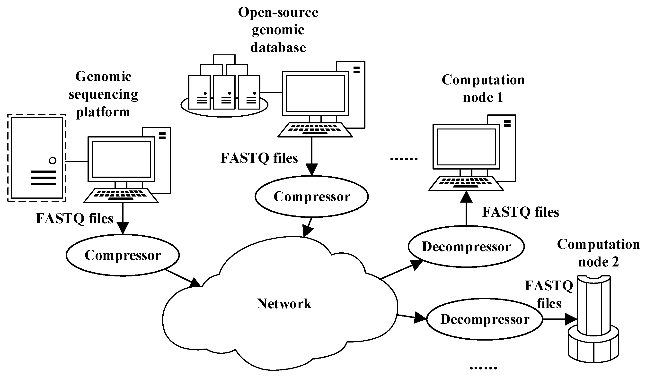
Compression algorithms can address these challenges by reducing the volume of genomic data (an example is shown in Figure 1). The compression result is transmitted by the network, while decompression is used to recover the files when genomic data analysis is requested by computation nodes. Currently, the volume of genomic data generated by high-throughput sequencing platforms or those downloaded from open-source genomic databases has reached GB or even TB level [16,17,18]. Furthermore, a NovaSeq X NGS platform can generate 8Tbase output in about 17–48 h [18]. It takes minutes, even hours [19,20,21], for the current available CPU-based compression algorithms to compress and decompress. For example, the algorithm in [20] used 10 min to compress a 7708 MB genomic file. The long processing time reduces the overall analysis system performance. Therefore, the acceleration of compression and decompression would be beneficial.

Online compression and decompression [22,23,24] can process data streams simultaneously with their input. FPGA (field-programmable gate array) is known for its support of high parallelism, flexible programming, and excellent real-time processing. These features make FPGA an ideal platform for implementing online compression algorithms. High parallelism helps increase the processing speed. Flexible programming enables special designs for genomic data to process input data faster and consume fewer power and hardware resources, which can help FPGA-based implementations easily embed in edge devices with limited resources and collaborate with existing FPGA-based data analysis algorithms [7,8,9,10,25,26,27].

FASTQ is a commonly used file format [17,19,20,21,28,29], with ‘.fastq’ as its suffix, for genomic data. Compression algorithms for FASTQ files can be categorized as either lossless or lossy. Although lossy compression can achieve higher compression ratios, it loses information after compression. This paper focuses on lossless compression for FASTQ files to maintain all the valid information.

LZ4 [30] and Zstd [31] are general lossless compression algorithms designed for fast compression, and they can be used to compress FASTQ files. The basic idea of such algorithms is to use contextual redundancy in a sliding window to achieve compression. However, the size of the sliding window is limited. The structural characteristics of FASTQ files determine that sliding windows often fail to capture much of the contextual redundancy.

Several lossless compression methods specifically designed for FASTQ files have been proposed. A reference probabilistic de Bruijn Graph, built de novo from a set of reads and stored in a Bloom filter, was used to compress sequencing data in [19]. Faraz Hach designed SCALCE, a ‘boosting’ scheme based on the Locally Consistent Parsing technique, to achieve FASTQ compression in [20]. Shubham Chandak developed a FASTQ compressor with multiple compression modes called SPRING in [21]. These algorithms are performed by CPU and can achieve a good compression ratio. However, their compression processes suffer from low throughput rates and high CPU occupation. It usually takes minutes (even hours), large memory, and multiple CPU cores for them to compress GB-level FASTQ files. Therefore, these algorithms can not achieve online compression.

J. Arram proposed a reference-based genomic alignment (REBA) method to perform genomic compression on FPGA in [16]. This method can achieve a better compression ratio than reference-free compression algorithms. ‘Reference-based’ algorithms require a genome sequence reference used as a dictionary to compress, while ‘reference-free’ algorithms do not need a genomic reference. However, storing the reference sequence and frequent memory access consume a great deal of power and hardware resources. In addition, looking up in the reference introduces unpredictable latency, which limits its throughput rate. The high resource and power consumption decrease the flexibility and reusability of the algorithm, which makes further parallel implementation difficult. Moreover, the decompression method was not proposed in [16].

In summary, when facing the challenge of online compression for genomic data, current genomic compression algorithms present several limitations:

• The CPU-based general and genomic-specific compression algorithms typically occupy multiple CPU cores while delivering limited processing speed. Therefore, these algorithms cannot achieve online compression and decompression.
• The FPGA-based general and reference-based compression algorithms tend to consume significant memory resources and require frequent memory access. Furthermore, our evaluations reveal that FPGA-based general-purpose compression algorithms yield suboptimal compression ratios when applied to FASTQ files.
• Existing studies primarily emphasize the acceleration of compression algorithms, with little attention given to the optimization or acceleration of decompression algorithms.

To address these issues, we propose PLORC, a novel Pipelined Lossless Reference-free Compression architecture, comprising both a compressor and a decompressor, specially designed for streaming genomic data in a FASTQ format. The main contributions of our work are as follows:

• We designed a fully pipelined architecture of the compressor and decompressor for streaming genomic data in a FASTQ format. All the modules were specially designed and built according to the structure of FASTQ files and the features of FPGA. As far as we know, PLORC is the first FPGA-based pipelined reference-free FASTQ compression architecture.
• The PLORC compressor achieved the best throughput rate among the representative algorithms we tested, while the decompressor matched the high throughput rate, maintaining balanced performance.
• PLORC demonstrated superior resource utilization and power efficiency compared to the FPGA-based algorithms evaluated in this study.
• The PLORC compressor surpassed some common general-purpose algorithms in terms of the compression ratio.

This paper is organized as follows: Section 2 provides a detailed explanation of the PLORC compressor and its hardware implementation. Section 3 discusses the PLORC decompressor and its corresponding hardware architecture. Section 4 presents the experimental results and discusses the findings. Finally, Section 5 concludes the paper and outlines directions for future work.

2. Proposed Compressor

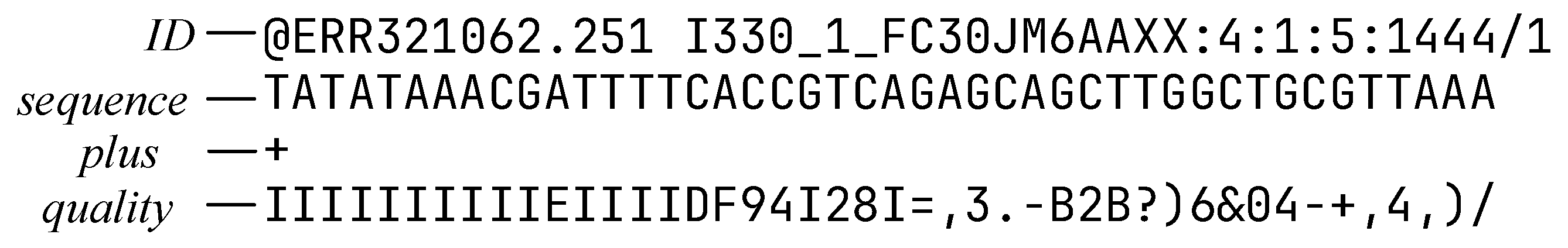
FASTQ files consist of fundamental data units called reads. Each read includes four parts [32] (as depicted in Figure 2): ID, sequence, plus, and quality. The sequence part represents the nucleotide bases. The quality part indicates the error probability of the bases. The plus part serves as a delimiter.

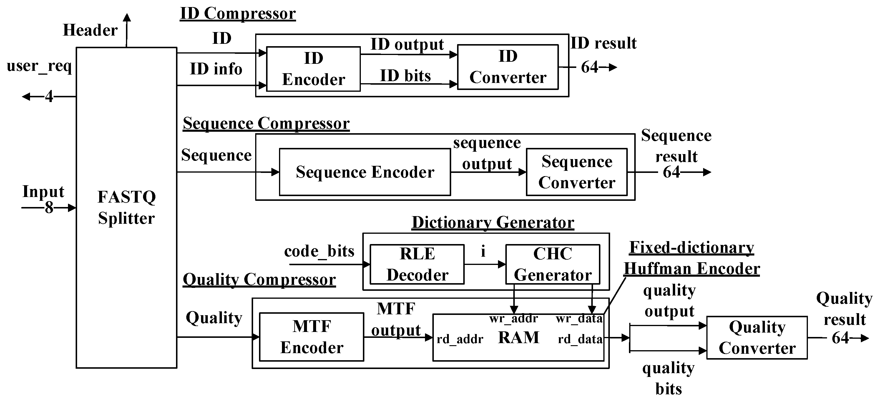
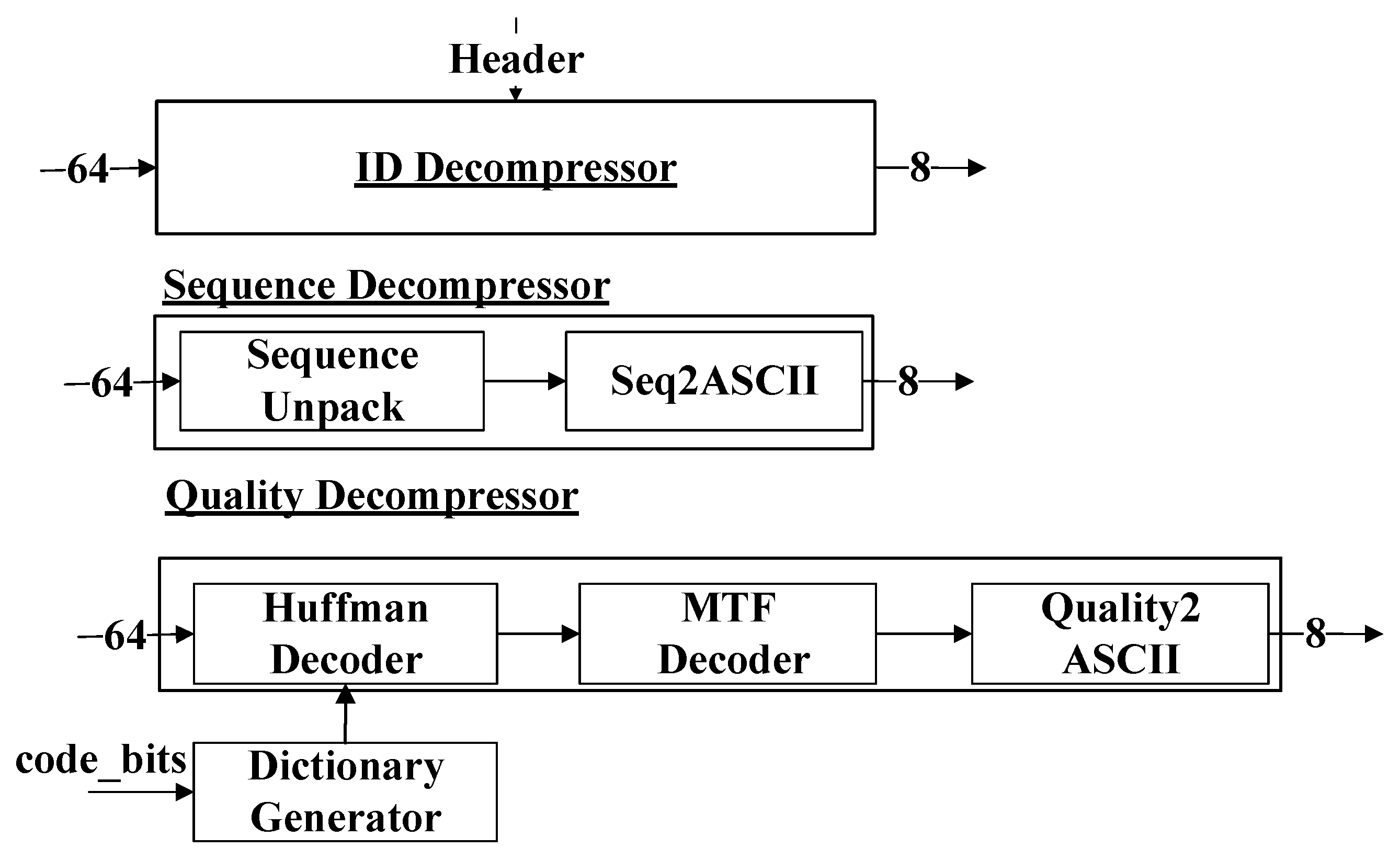
The block diagram of our proposed compressor is shown in Figure 3. The input of our compressor is in the format of an 8-bit ASCII (American Standard Code for Information Interchange) code stream. The compressor consists of seven modules: the FASTQ Splitter, the ID Compressor, the Sequence Compressor, the Quality Compressor, the ID Converter, the Sequence Converter, and the Quality Converter. ‘ID output’, ‘sequence output’, and ‘quality output’ stand for the compression results. ‘ID bits’ and ‘quality bits’ represent the number of valid bits in ‘ID output’ and ‘quality output’. The ‘code_bits’ signal represents a stream of the length of Huffman code words. The output is then processed by the three converter modules, respectively, to extract the valid information and form 64-bit output streams.

2.1. The FASTQ Splitter Module

The FASTQ Splitter module is responsible for the following:

• Dividing the input data stream into three output streams. The three compressors receive the streams and perform compression processes, respectively.
• Generating the header and ‘ID_info’ signal, as shown in Figure 3. The FASTQ Splitter extracts (1) the length of the first ID, (2) the content of the first ID, and (3) the positions, type, and amount of the special characters other than the numbers and English letters in the first ID. The information is transformed into the header and ‘ID_info’.
• Handling some exceptional situations and requesting user intervention. The module detects the exceptional situations and sets the corresponding bit as one in ‘user_req’ to call for user intervention. The information about ‘user_req’ is listed below:

  –

  The ‘user_req[0]’ notation represents the occurrence of ambiguous bases other than ‘A’, ‘C’, ‘G’, ‘T’, and ‘N’.

  –

  The ‘user_req[1]’ notation determines that the number of quality scores is different from the bases in the current read.

  –

  The ‘user_req[2]’ notation means a mismatch between the type or amount of special characters in the first read and the current read.

  –

  The ‘user_req[3]’ notation means some of the four parts are missing in the current read.

2.2. The ID Encoder Module

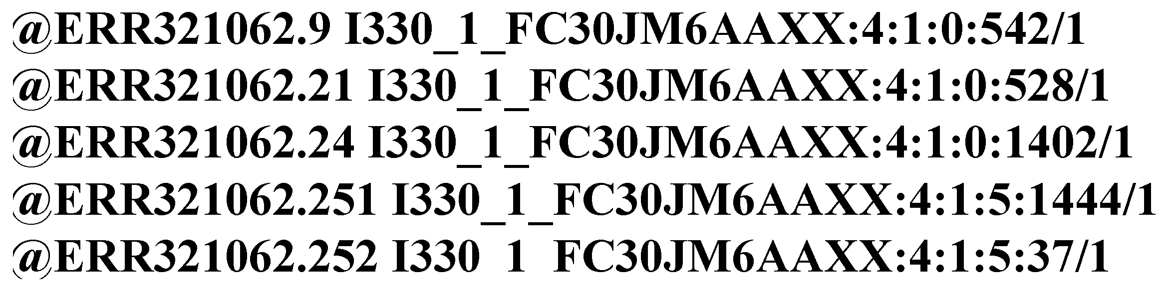
Figure 4 shows an example of IDs randomly selected from a FASTQ file. The characters in an ID can be divided into two categories:

• Numbers and English letters.
• Special characters other than numbers and English letters, such as ‘@’, ‘:’, and space.

The IDs from a FASTQ file are of a identical format [33]. Each ID is divided into several areas by special characters. The areas contain different information about this read. The differences between these IDs are merely a few symbols. Therefore, the IDs from the same FASTQ file show high structural similarity.

We designed an encoding method based on character comparison utilizing structural similarity. The method divides the character comparison process into eight different input patterns and employs different strategies. We used segments in the comparison to illustrate the strategies. The segments are shown in Figure 5 and Figure 6. The patterns in Figure 6 are the special cases of those in Figure 5. They are defined as ‘special patterns’ because they require special treatments compared with common patterns.

The ‘base_ID’ stores the ID from the previous read to participate in the comparison. For the first read, the ‘base_ID’ is itself extracted by the FASTQ Splitter module. The length of the ‘base_ID’ in bytes is also stored. The ‘input_ID’ represents the streaming ID input. The ‘base_ptr represents which symbol in the ‘base_ID’ is participating in the comparison, which is named ‘c_base’. The character from the ‘input_ID’ is referred to as the ‘c_input’. The first 4 bits of the result are the difference between the length of the current input ID and the previous ID in bytes, which is called the ‘len_diff’.

The encoding process decides which pattern the current comparison between the ‘c_base’ and ‘c_input’ belongs to and then applies the corresponding strategy.

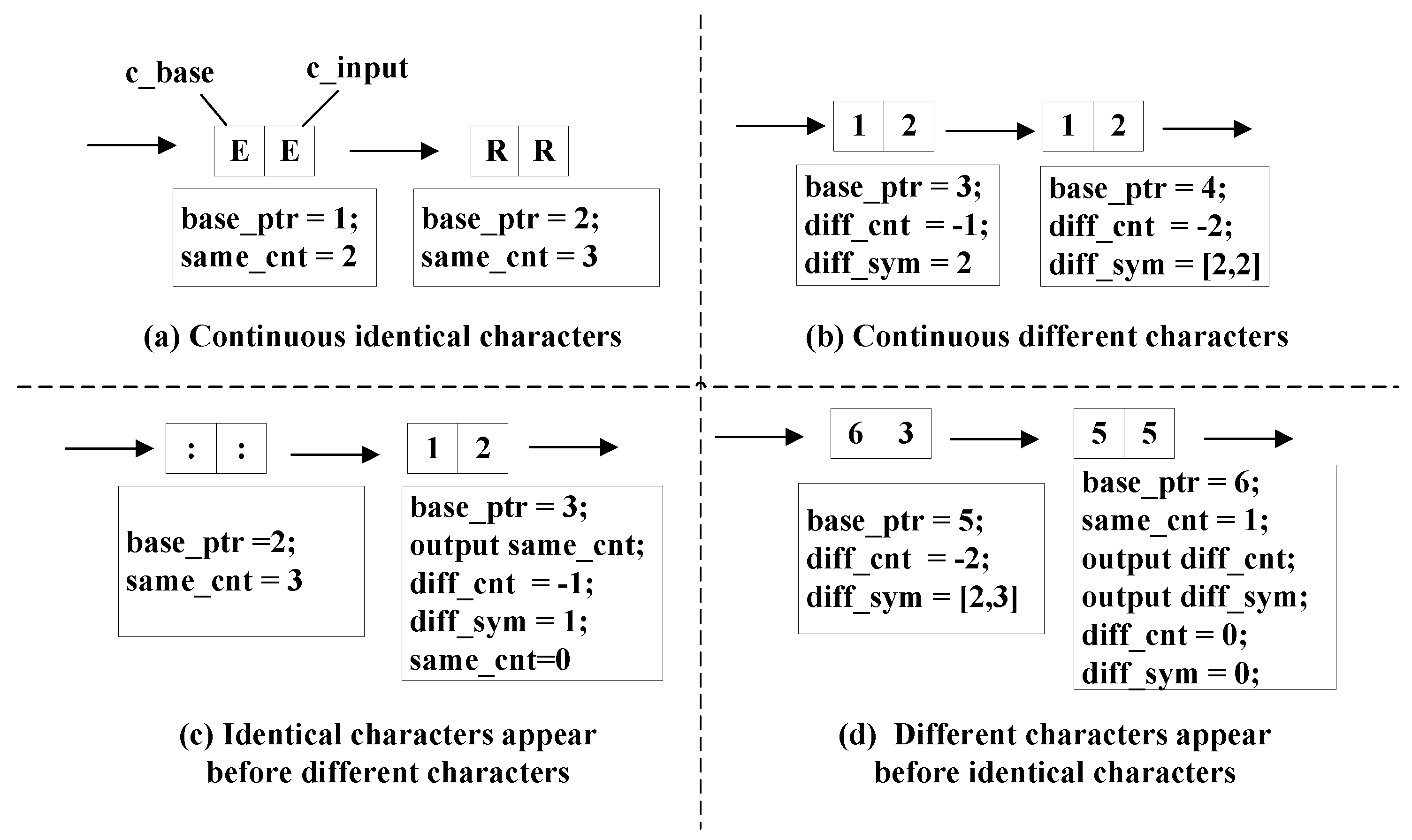
The strategies for common patterns shown in Figure 5 are listed below.

• In Figure 5a, there are continuous identical characters. A 1-byte register named ‘same_cnt’ is used to store the number of identical characters.
• In Figure 5b, there are continuous different characters. Another 1-byte register ‘diff_cnt’ calculates the number of different characters. Its value is negative to separate itself from the ‘same_cnt’ register. The ‘diff_sym’ register stores the input character. The number of characters contained in ‘diff_sym’ is recorded for future output.
• In Figure 5c, a pair of identical characters appear before different characters. The comparison status is changed. Therefore, the value of ‘same_cnt’ becomes the output signal ‘ID output’ in Figure 3 and is then set as zero. The ‘ID bits’ is 8 because ‘same_cnt’ is a 1-byte register.
• In Figure 5d, a pair of different characters appear before identical characters. The output is generated from ‘diff_sym’ nad ‘diff_cnt’.

The strategies for special patterns shown in Figure 6 are listed below.

• In Figure 6a, the ‘c_base’ becomes a special character before ‘c_input’. It is a special case of Figure 5d, and it means the same special character will appear after some characters in input_ID because of the high structural similarity. The base_ptr should remain unchanged. The ‘diff_sym’ and ‘diff_cnt’ are required to update continuously until the special character in ‘input_ID’ arrives. The following operations are the same as in Figure 5d.
• In Figure 6b, the ‘c_input’ becomes a special character before ‘c_base’. This pattern is also a special case of Figure 5d. The difference between the situations shown in Figure 6a,b is are the same as that in Figure 6b, and the ‘c_input’ can not remain unchanged when waiting for the special character from ‘base_ID’ because it introduces stream interruption. Therefore, the ‘base_ptr’ should jump to the position of the next special character in ‘base_ID’. The position is provided by the FASTQ Splitter module. The other operations are the same as in Figure 5d.
• In Figure 6c, the ‘c_input’ reaches the end of ‘input_ID’ first. The encoder should generate the output immediately and set the ‘base_ptr’ to zero to wait for new inputs. If the comparison status before the end is a pair of identical characters, the output should be generated from ‘same_cnt’. Otherwise, the output should be generated from ‘diff_sym’ and ‘diff_cnt.
• In Figure 6d, the ‘c_base’ reaches the end of ‘base_ID’ first. Under this situation, the following characters from ‘input_ID’ should be treated as pairs of different characters because there is no character from ‘base_ID’ to participate in the comparison. The encoder is supposed to wait until the ‘input_ID’ reaches its end and then generate outputs from ‘diff_sym’ and ‘diff_cnt’.

An example is shown below to illustrate the encoding process on a real ID.

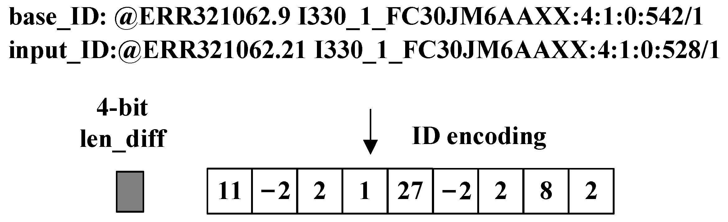
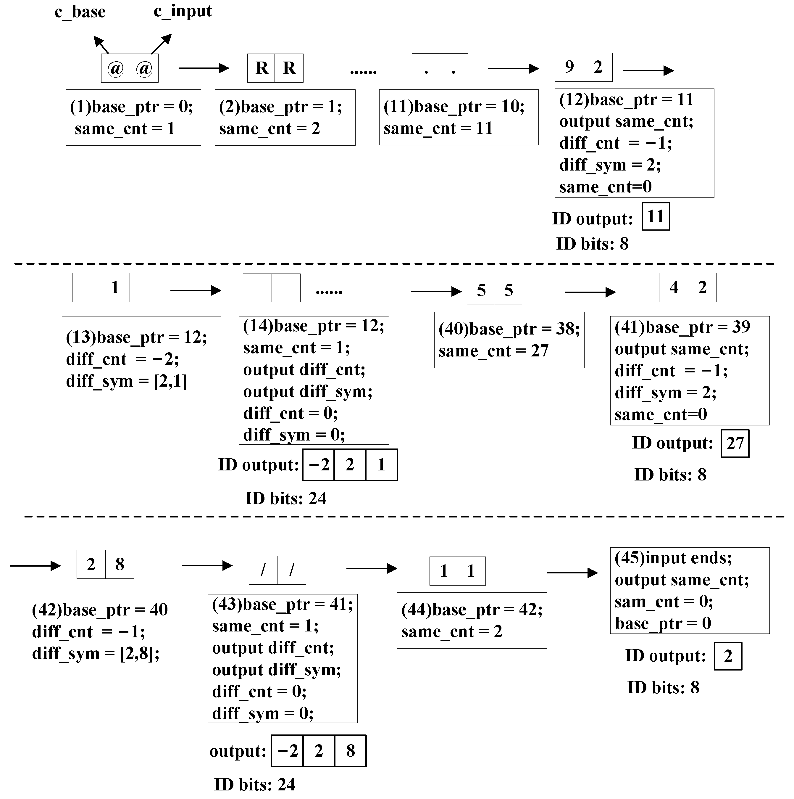
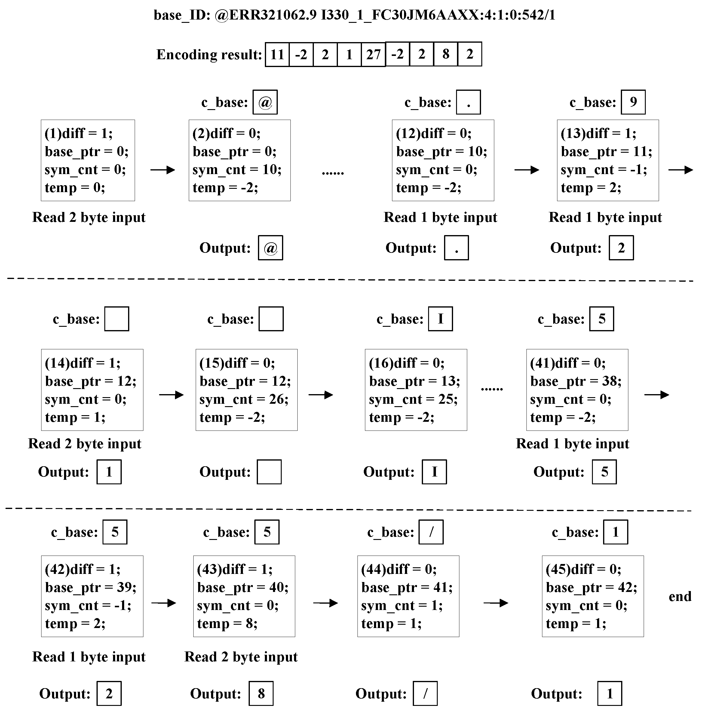
Figure 7 shows an example of a real ID encoding result. Its encoding process is shown in Figure 8. The white blocks in Figure 7 and Figure 8 represent 1-byte data. Our encoding method turns 44 bytes ‘input_ID’ into a 9.5-byte encoding result, including a 4-bit ‘len_diff’.

In Figure 8, ‘c_base’ means a character from ‘base_id’, and ‘c_input’ means a character from ‘input_id’. The value of ‘c_base’ changes with ‘base_ptr’ and the ‘c_input’ changes with the input stream.

• The encoder first generates the ‘len_diff’ from the difference between the length of the current input ID and the previous ID in bytes. The ‘c_input’ character in each step is stored, and the number of ‘c_input’ characters is recorded by registers to update the ‘base_id’ at the end of the current comparison.
• From Step (1) to Step (11) in Figure 8, the encoder encounters continuous identical characters, as shown in Figure 5a. The ‘same_cnt’ and ‘base_ptr’ registers the increase by one in each step.
• The encoder encounters a pair of identical characters in Step (11) and then different characters in Step (12), as shown in Figure 5c. Therefore, the ‘ID output’ signal is generated from ‘same_cnt’. Meanwhile, ‘diff_sym’ and ‘diff_cnt’ begin to update.
• In Step (12) and Step (13), the encoder encounters continuous different characters, as shown in Figure 5b. Then, ‘diff_sym’ and ‘diff_cnt’ resisters continue to update.
• The value of register ‘c_base’ becomes a special character in Step (13) first, as shown in Figure 6a. The ‘c_base’ register remains unchanged until the special character from ‘input_id’ arrives in Step (14). The ‘ID output’ signal is generated from ‘diff_sym’ and ‘diff_cnt’.
• From Step (14) to Step (40), the encoder encounters continuous identical characters again. Then, ‘same_cnt’ and ‘base_ptr’ register the increase by one in each step.
• The encoder encounters a pair of identical characters in Step (40) and a pair of different characters in Step (41). The pattern is the same as Step (11)–(12).
• In Step (41) and Step (42), the encoder encounters continuous different characters. The pattern is the same as Steps (12)–(13).
• The encoder encounters a pair of different characters in Step (42) and identical characters in Step (43), as shown in Figure 5d. The ‘ID output’ signal is generated from ‘diff_sym’ and ‘diff_cnt’. Meanwhile, ‘same_cnt’ begins to update.
• In Steps (43) and (44), the encoder encounters continuous identical characters the third time. The operations are the same as Steps (1)–(11).
• In Step (45), ‘c_input’ reaches the end first, as shown in Figure 6c. The outputs are generated, and all the registers are set to zero. Then, ‘base_ID’ and its size are updated by the ‘input_ID’ in the finished comparison and its length in bytes.

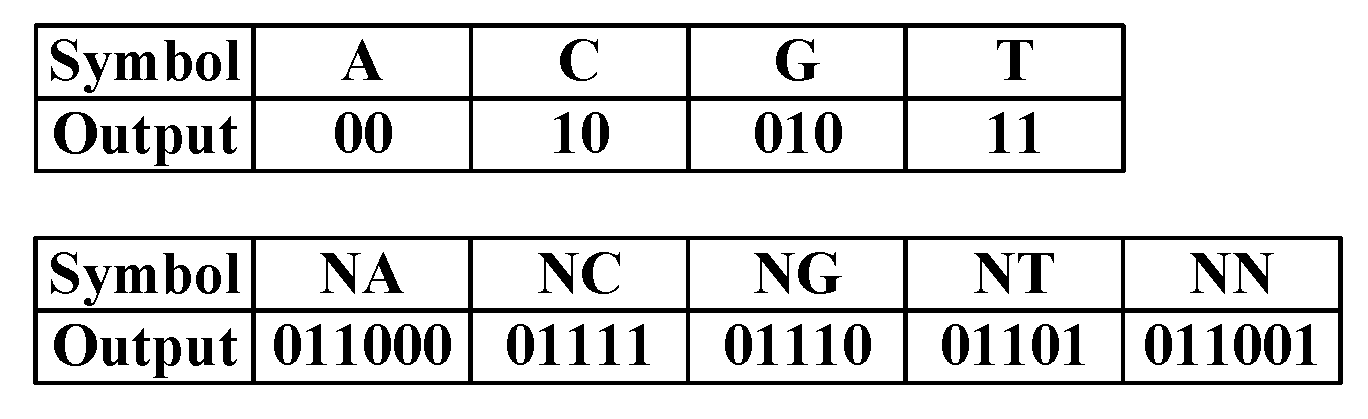
2.3. The Sequence Compressor Module

Sequences are composed of four nucleotide bases: ‘A’, ‘C’, ‘G’, and ‘T’. In addition, the character ‘N’ indicates an ambiguous base in the sequence. We used a Huffman code table to encode the sequence part losslessly, as shown in Figure 9. During the encoding, the code table is unchanging.

The number of bases in the sequence part is calculated and serves as the first 2 bytes of the ‘sequence output’ of each read.

2.4. The Quality Compressor Module

There are merely 41 types of characters in the quality part [34]. The distribution pattern of the quality part is that characters corresponding to higher sequencing accuracy tend to occur with higher frequency [35]. Figure 10 shows the frequency distribution of characters based on the first 1000 reads of ERR174310_1.fastq. The x-axis represents the rank of the occurrence frequency of the characters in descending order. The y-axis represents the percentage of the character.

Table 1. The percentage of the top five characters in quality characters from ERR174310_1.fastq in terms of appearance frequency.

Rank	Symbol	p_error	%
1	J	0.00008	23.86
2	I	0.00010	12.33
3	H	0.00013	10.17
4	F	0.00020	9.02
5	D	0.00032	8.78

shows the percentage of the top five characters in terms of appearance frequency, where p_error means the probability of error. This distribution pattern can be used to simplify the compression process.

Given the distribution pattern shown in Figure 10, entropy encoding can achieve appreciable compression performance. Among the entropy encoding methods, Huffman encoding can be easily realized by FPGA devices using RAMs. Therefore, an optimized Huffman encoding process is used in the Quality Compressor module.

The structure of the Quality Compressor is shown in Figure 3.

The hardware details of the submodules are discussed below.

2.4.1. The MTF Encoder Module

We apply the MTF (move-to-front) transform [36] to turn the characters into numbers. An example of the MTF encoding process is shown in

Table 2. An example of MTF encoding.

Input	Stack	Output
1	[0,1,2]	1
0	[1,0,2]	1
2	[0,1,2]	2
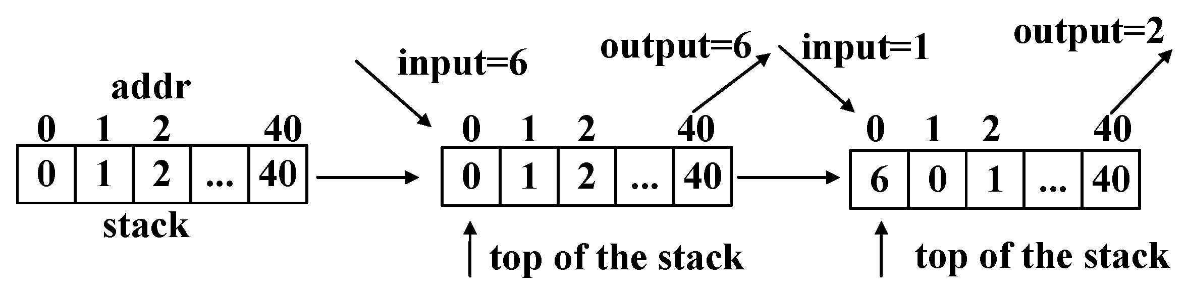
2	[2,0,1]	0
2	[2,0,1]	0

. A stack is maintained to achieve the encoding process. The stack is initialized with incremental integers, starting from 0. The first input signal is 1. This input signal is then looked up in the stack, and its address is returned as the output signal. Element 1 is then moved to the top of the stack. The second input signal is 0. According to the above process, the corresponding output signal is 1. An example of the MTF encoding for quality parts is shown in Figure 11. The basic encoding method is the same as in Table 2.

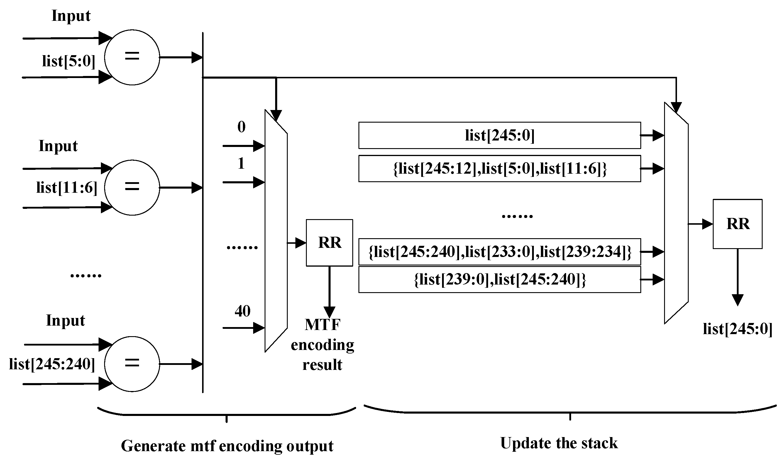
The architecture of the MTF Encoder module is shown in Figure 12. The $list$ signal is the stack in the MTF Encoder module. ‘RR’ means ‘register’ in Figure 12.

The MTF Encoder transforms those characters that appear more frequently into smaller integers.

Table 3. The distribution of the MTF input and results.

FASTQ File	ERR174310_1		SRR554369_2
Rank	MTF Input	MTF Results	MTF Input	MTF Results
1	23.86%	43.73%	36.63%	41.50%
2	13.33%	15.98%	10.28%	16.14%
3	10.17%	8.07%	9.2%	9.11%
total	47.36%	67.78%	56.11%	66.75%

shows the MTF encoding input and results on ERR174310_1.fastq and SRR554369_2.fastq, where the percentage of the first, second, and third most frequent characters and their sums are listed. As shown in Table 3, the sum of the percentage of the top 3 characters is increased after MTF encoding. Additionally, the percentages of the top 2 characters are both increased by MTF.

2.4.2. The Dictionary Generator Module

The structure of the Dictionary Generator is shown in Figure 3. It transforms the Huffman code word length values into the corresponding Huffman code table. The code word length values are set by the users before the compression. The Huffman code table remains unchanged during the compression process.

We introduce Canonical Huffman Coding (CHC) [37,38,39] to simplify the transmission of the Huffman dictionary. CHC allows generating binary Huffman codes $f\left(i\right)$ from the Huffman code length i and several rules. These rules are listed below.

• The codes with the same length are consecutive integers in binary format.
• The first code $f\left(i\right)$ of length i can be calculated from the last code of length $i-1$, which can be expressed as $f\left(i\right)=\left(f\right(i-1)+1)\times 2$.
• The first code with the smallest length starts from 0.
• If $f(i+1)$ does not exist after $f\left(i\right)$, and the nearest code word is $f(i+k)$, then $f(i+k)=(f\left(i\right)+1)\times 2^k$.

The Dictionary Generator module consists of two submodules: the RLE Decoder module and the CHC Generator module.

Since consecutive identical code length values occur frequently, the code length values are encoded as the ‘code_bits’ signal with the RLE method.

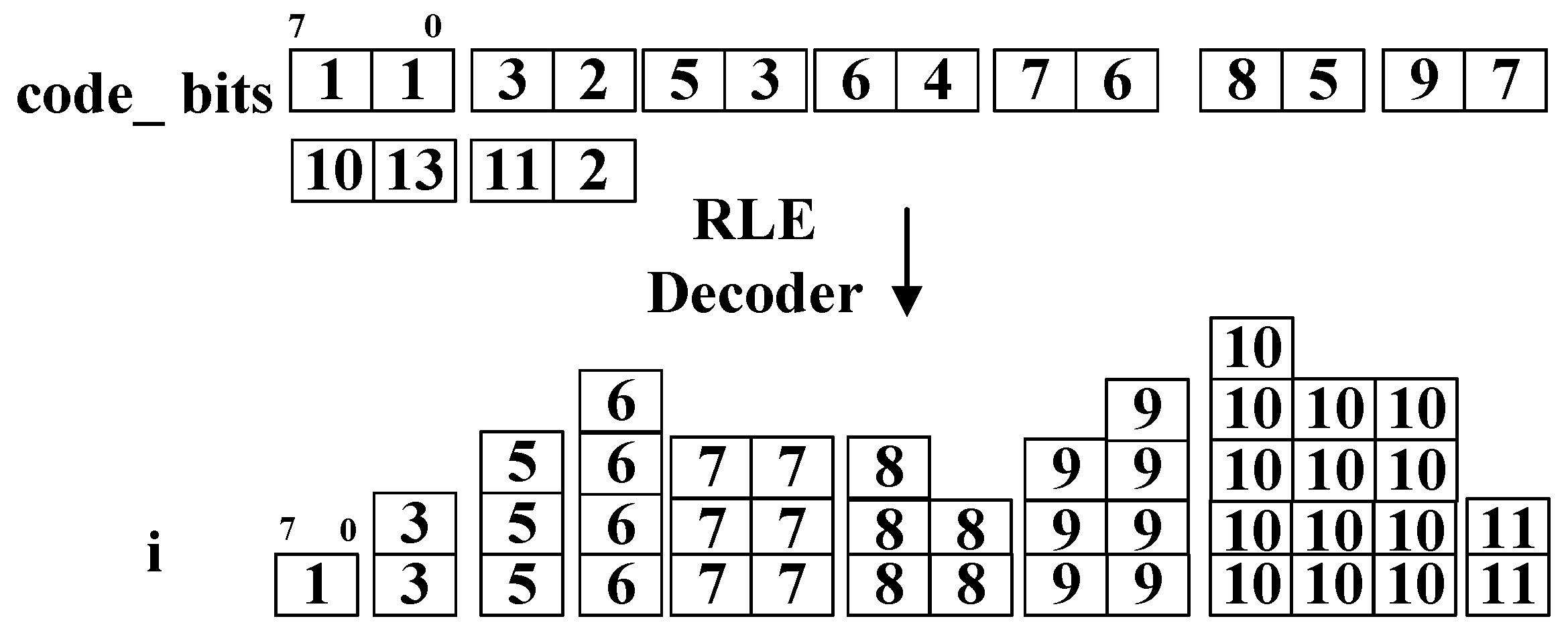
The RLE Decoder module generates the code length i from the ‘code_bits’ signal. An example of the input and output of the RLE Decoder module is shown in Figure 13, where the total size of ‘code_bits’ is 9 bytes and the total size of i is 43 bytes. A smaller volume of the input saves time in configuring the Huffman encoder.

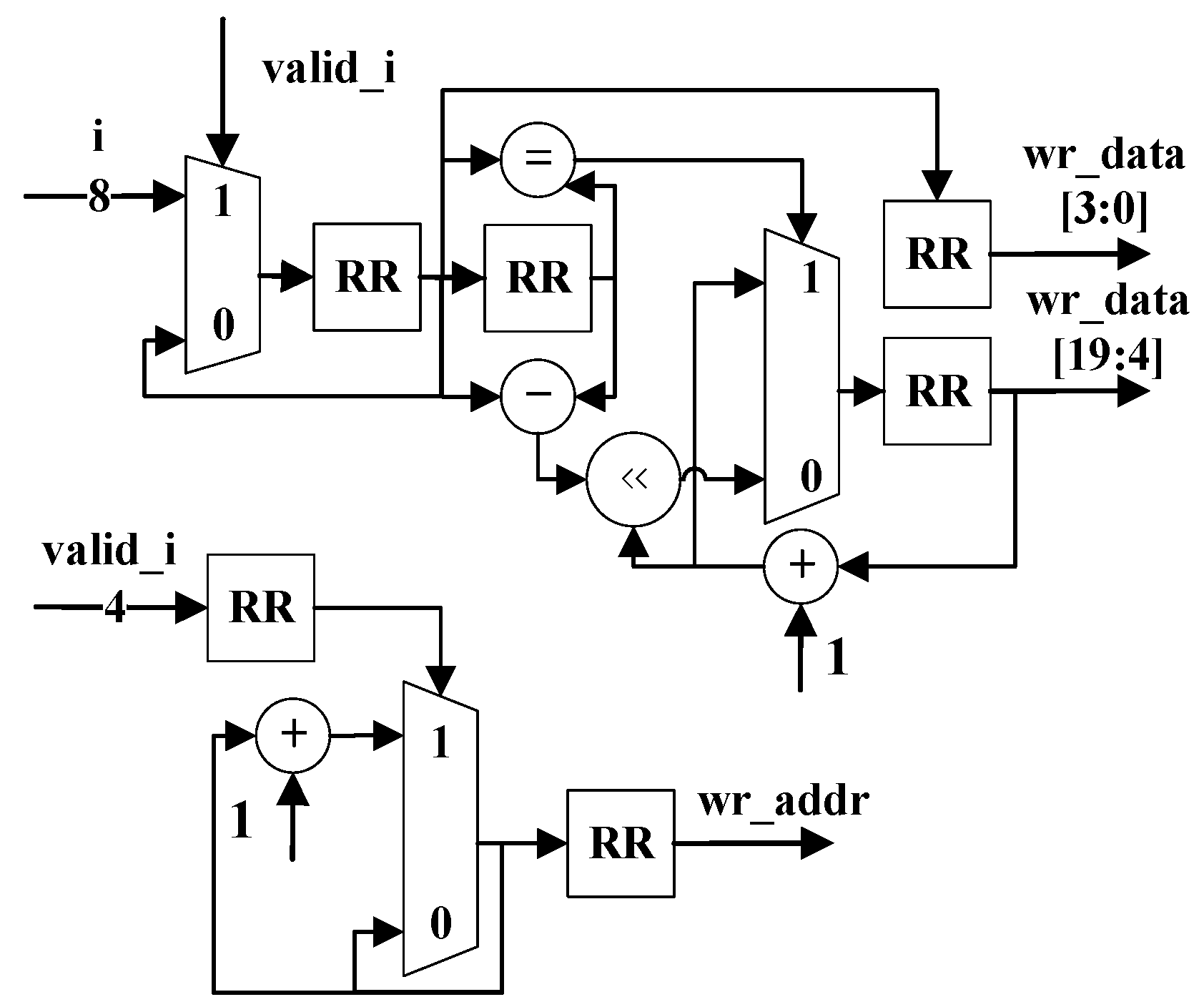
The CHC Generator module transforms the code word length i into the code table $f\left(i\right)$. Its architecture is shown in Figure 14. ‘RR’ means ‘register’ in Figure 14. Its input i is the output of the RLE Decoder module. Its output $wr\_addr$ and $wr\_data$ are served as the input of the fixed-dictionary Huffman Encoder module. In Figure 14, $wr\_data[19:4]$ represents the Huffman code table and $wr\_data[3:0]$ means the amount of valid bits in $wr\_data[19:4]$.

2.4.3. The Fixed-Dictionary Huffman Encoder Module

The traditional Huffman encoding consists of two phases: constructing a Huffman tree, and encoding based on the tree. This scheme requires the nodes on the tree to be scanned twice, which results in a longer encoding time [39]. The construction of a Huffman tree consumes 38% of the total encoding time [40]. In addition, the FPGA implementation of the Huffman tree construction process needs extra memory [41].

To avoid the latency and resource overhead of constructing a Huffman tree, we omitted the Huffman tree construction process and utilized a fixed-dictionary Huffman encoder. Based on the observed character frequency distribution in Figure 10 and Table 3, applying fixed-dictionary Huffman encoding will lose little compression ratio. Additionally, this modification enables pipelined and resource-efficient implementation of the Huffman encoding process.

The fixed-dictionary Huffman Encoder module consists of a RAM (Random Access Memory). The Huffman dictionary generated by the Dictionary Generator module is written in RAM. The Huffman encoding process is implemented by reading the RAM with the ‘MTF output’ signal as the reading address.

2.5. The ID, Sequence, and Quality Converter Modules

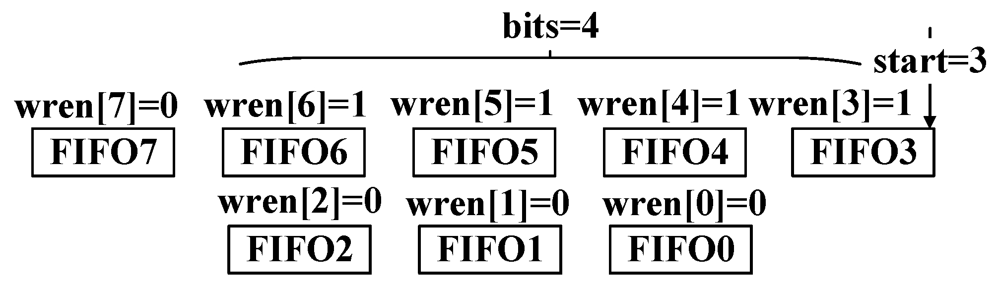
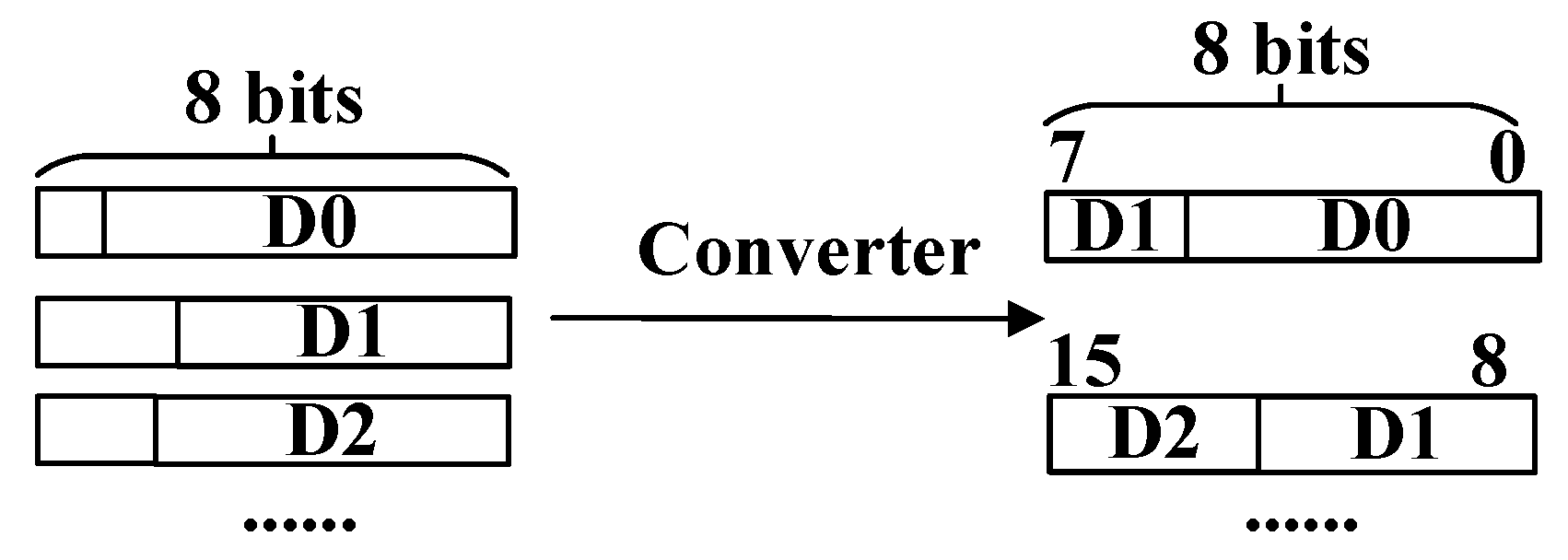
The ID Converter, Sequence Converter, and Quality Converter collect the valid bits in the input and transform these bits into output with a unified bit width. All modules utilize parallel 1-bit width FIFOs to achieve this transformation, as shown in Figure 15. Figure 16 shows the process of transforming the data less than eight bits into eight bits. The input signals are D0, D1, and D2 with a bit width of less than 8 bits. To illustrate their hardware structure, the output bit width of the package module is set as eight bits, as is shown as examples in Figure 15 and Figure 16.

Figure 15 shows the hardware architecture of the converter. The input contains 4-bit valid data and should be written starting from FIFO3. Moreover, ‘bits’ indicates the number of valid bits in the input data. Only these valid bits can be written into FIFOs. Furthermore, ‘start’ means where this writing process should begin. Reading these FIFOs when they are not empty simultaneously can form an 8-bit signal. The actual output is set to a 64-bit width in the experiments. The 64-bit (8 bytes) width is convenient for further storage and calculation of the compression output. Other output widths can be easily transformed from the 64-bit output.

3. Proposed Decompressor

The proposed decompressor is illustrated in Figure 17. The input consists of 64-bit compressed data, while the output is an 8-bit ASCII code stream. The decompression process is symmetric to the compression process.

3.1. The ID Decompressor Module

The ID decompression process is symmetric to the ID encoding process. We used the example from Figure 7 as the decoding input and output to illustrate the decoding strategies. The decoding process is shown in Figure 18.

In Figure 18, ‘c_base’ is the character in the ‘base_ID’ pointed by ‘base_ptr’. The ‘sym_cnt’ register represents the number of characters that need decoding, and ‘temp’ is a register for the unused byte from the ID compression result. These registers are 1-byte registers. The 1-bit ‘diff’ register represents whether the output is identical or different characters. The length of the compressed ID is calculated from the 4-bit ‘len_diff’.

The most important register in the module is ‘diff’. The 1-bit value of ‘diff’ changes when ‘sym_cnt’ is zero. A classification of the operations in Figure 18 is shown in

Table 4. A classification of the operations in Figure 18.

‘diff’	0	1
How many bytes should be	Read 1 byte when ‘sym_cnt’ = 0;	Read 2 bytes when ‘sym_cnt’/ = 0;
read	otherwise read no byte.	otherwise read 1 byte.
	example: Steps (12) and (41).	Example: Steps (1), (14), and (43).
The source of the	Output = ‘c_base’.	Output = ‘temp’.
output characters	Example: Step (2)–(12), (15)–(41), and (44)–(45).	Example: Steps (13), (14), (42), and (43).
How to update	‘sym_cnt’ = ‘temp’;	(a) if one byte is read,
‘sym_cnt’ and ‘temp’	then ‘temp’ = new input.	‘sym_cnt’ = ‘sym_cnt’-1;
after reading input bytes	Example: Steps (12) and (41).	‘temp’ = new input.
		(b) if two bytes are read,
		‘sym_cnt’ = the first byte,
		‘temp’ = the second byte.
		Example for (a): Steps (13) and (42);
		Example for (b): Step (1), (14), and (43).

. The steps from Figure 18 are given as examples in the table.

A discussion about some of the special situations in Figure 18 is listed below.

• In Step (14), ‘c_base’ becomes a space character. Furthermore, ‘base_ptr’ remains unchanged. When ‘diff’ is zero, it means the special character identical to ‘c_base’ is read from the encoding result. Then, ‘base_ptr’ begins to change.
• After Step (45), this decoding process reaches its end. The end is determined by the length value of this ID generated from ‘len_diff’. The last character of the decoding result is a linefeed symbol inserted by the decoder. The decoder updates base_id using the decoded ID result to participate in the next decoding process.

3.2. The Sequence Decompressor Module

The decompression for the sequence part is first extracting the first 2 bytes of the sequence encoding result as the length of this sequence. The decoding process is a Huffman decoding process, according to the encoding table in Figure 9. The architecture of the Huffman decoding is discussed in Section 3.3.1. The encoding table is contained in the architecture.

A look-up table is applied in the Seq2ASCII module to transform the Huffman decoding output into ASCII format. When the amount of output reaches the length of this sequence, a linefeed character and a plus character are set as outputs to recover the FASTQ structure [32].

3.3. The Quality Decompressor Module

3.3.1. The Huffman Decoder Module

The primary challenge in the Huffman decoding process is to extract Huffman code words from the input. The Huffman encoding results are of two features:

• Huffman code words are prefix codes, which means each code is not the prefix of the other codes.
• A 16-bit width is enough for Huffman code words because of the limited types of characters.

These two features allow parallel comparisons between the Huffman decoding input and the Huffman Dictionary items to expedite processing.

Two kinds of registers are generated from the Huffman dictionary:

• ‘code_times[i]’: an 8-bit width register that specifies the number of Huffman code words with i-bit length.
• ‘code_start[i]’: the starting code for i-bit length Huffman code words.

If no i-bit length Huffman code word exists, these registers hold a value of 0. For example, the ‘code_times[i]’ and code_start[i]’ generated from the Huffman code table in Figure 13 are listed in

Table 5. The information generated from the Huffman code word length example.

i	code_start[i]	code_times[i]	i	code_start[i]	code_times[i]
	(hex)	(dec)		(hex)	(dec)
1	0x0	1	9	0x1f2	7
2	0x0	0	10	0x3f2	13
3	0x4	2	11	0x7fe	2
4	0x0	0	12	0x0	0
5	0x18	3	13	0x0	0
6	0x36	4	14	0x0	0
7	0x74	6	15	0x0	0
8	0xf4	5	16	0x0	0

. The ‘code_times[i]’ values are in decimal format. The prefix ‘0x’ means the ‘code_start[i]’ values are in hexadecimal format.

Algorithm 1 outlines the comparison process. The Huffman decoding input is stored in a register named ‘bytes’. The ‘diff[i]’ values and the comparison processes can be performed concurrently in the FPGA implementation.

Algorithm 1 Finding the Huffman encoding result.

1:  for $i\leftarrow 1,16$ do   2:        diff[i] ← bytes[0:i-1] - code_start[i]   3:        if $0<=$ diff[i] < code_times[i] then   4:           break;   5:        end if   6:  end for   7:  bytes[0:i-1] is a Huffman encoding result.

Figure 19 shows an example of the Huffman decoding process, where ‘start’ represents where the Huffman code begins, and ‘addr’ means the start address of the Huffman encoding results. Algorithm 1 shows how to look up a symbol in the Huffman dictionary.

Another Huffman decoding process example is listed in

Table 6. An example of the Huffman decoding process.

i	bytes[0:i-1]	code_start[i]	code_times[i]	diff[i]
	(hex)	(hex)	(dec)	(dec)
1	0x1	0x0	1	1
2	0x2	0x0	0	2
3	0x4	0x4	2	0
4	0x9	0x0	0	9
5	0x12	0x18	3	−6
6	0x25	0x36	4	−17
7	0x48	0x74	6	−41
8	0x97	0xf4	5	−93
9	0x12e	0x1f2	7	−196
10	0x25c	0x3f2	13	−406
11	0x4b8	0x7fe	2	−838
12	0x971	0x0	0	2417
13	0x12e3	0x0	0	4835
14	0x2620	0x0	0	9760
15	0x4b8c	0x0	0	19,340
16	0x9718	0x0	0	38,680

. The decoding input is ‘1001011100011001’. Only when i = 3, the condition in Algorithm 1 is satisfied. Therefore, ‘100’ is identified as a valid Huffman code.

3.3.2. The MTF Decoder Module

The MTF decoding process is symmetric to the encoding process. The example of the MTF decoding process is shown in Figure 20.

The input represents an address in the stack, while the output is the content located at that address. The element indicated by the input address is moved to the top of the stack when the output is generated.

3.3.3. The Quality2ASCII Module

The Quality2ASCII module converts the MTF decoding results into their ASCII code. Due to the limited character set used in the quality part [34], this conversion can be efficiently implemented using look-up tables.

3.3.4. The Dictionary Generator Module

The Dictionary Generator module in the Quality Decompressor is identical to that used in the Quality Compressor module.

4. Results and Discussion

4.1. Datasets

The datasets used in this study [42,43,44,45,46] comprise publicly available paired-end FASTQ files obtained from EMBL-EBI [17]. These datasets encompass a wide range of DNA information from species and organisms, with the specific details provided in

Table 7. The description for tested fastq files.

Dataset
Number	Name	Organism	Size (GB)
1	ERR174310_1.fastq [42]	Human	50.1
2	ERR174310_2.fastq [42]		50.1
3	ERR321062_1.fastq [43]	Human gut metagenome	1.58
4	ERR321062_2.fastq [43]		1.58
5	SRR327342_1.fastq [44]	Saccharomyces cerevisiae	2.61
6	SRR327342_2.fastq [44]		2.95
7	SRR554369_1.fastq [45]	Pseudomonas	0.35
8	SRR554369_2.fastq [45]		0.35
9	SRR870667_1.fastq [46]	Theobroma cacao	17.2
10	SRR870667_2.fastq [46]		12.8

.

4.2. Experiment Information

We executed different compression algorithms on the FASTQ files listed in Table 7. As discussed in Section 1, CPU-based genomic-specific compression algorithms [19,20,21] have limited throughput rates. Therefore, these algorithms are not within the comparing scope of this article.

Our PLORC compressor and decompressor are implemented on a Zynq UltraScale+ ZCU102 Evaluation Board by Vivado 2022.2.

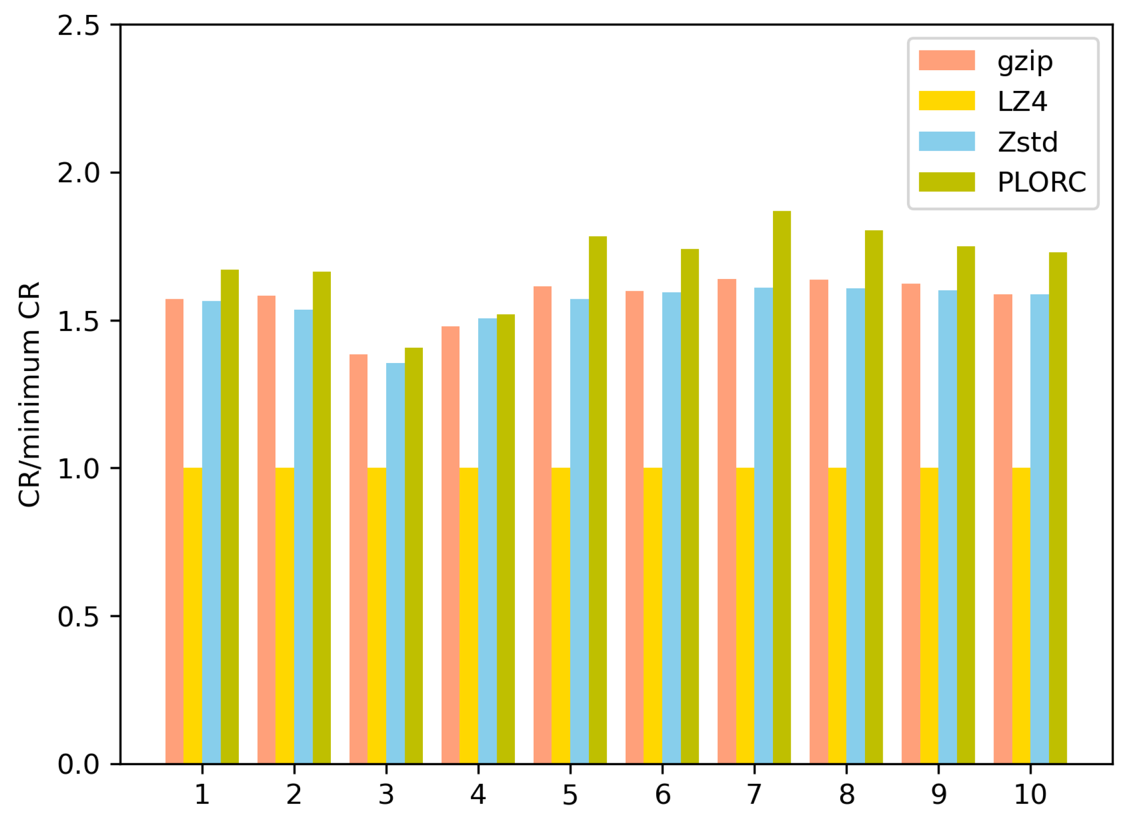
We conducted compression experiments on Gzip [47], LZ4 [30], and Zstd [31] to measure their CRs (compression ratios). The definition of CR is shown in Equation (1). The CRs of the tested compression algorithms are shown in

Table 8. The compression ratios of tested compression algorithms.

Dataset
Number	Gzip	LZ4	Zstd	PLORC
1 [42]	3.00	1.91	2.99	3.19
2 [42]	3.10	1.96	3.01	3.26
3 [43]	3.13	2.26	3.06	3.18
4 [43]	2.93	1.98	2.98	3.01
5 [44]	3.05	1.89	2.97	3.37
6 [44]	2.83	1.77	2.82	3.08
7 [45]	2.77	1.69	2.72	3.16
8 [45]	2.75	1.68	2.70	3.03
9 [46]	2.84	1.75	2.80	3.06
10 [46]	2.76	1.74	2.76	3.01

. A comparison of the CRs is shown in Figure 21. The x-axis of Figure 21 represents the ‘Dataset Number’ in Table 7. The y-axis means the ratio between the CR of the tested algorithm and the minimum CR on the same dataset. In addition, we implemented Gzip [48], LZ4, and Zstd [49] on a Zynq UltraScale+ ZCU102 Evaluation Board to measure their TPRs (throughput rates) and resource consumption.

The throughput rates and power consumption results of the FPGA-based algorithms are shown in

Table 9. The throughput rates and power consumption of the FPGA-based compressors.

	Gzip on FPGA 1	LZ4 on FPGA		Zstd on FPGA		REBA 2	PLORC
	Com 3	Com	Decom	Com	Decom	Com	Com	Decom
FPGA type	ZCU102	ZCU102	ZCU102	ZCU102	ZCU102	Stratix V	ZCU102	ZCU102
Power (W)	1.19	0.76	1.127	1.064	1.414	- 4	0.87	1.306
TPR (MB/s)	341	301	266	284	217	311 5	445	418
Pipeline Mode	Non-streaming	Non-streaming	Non-streaming	Non-streaming	Non-streaming	Non-streaming	Streaming	Streaming
PE ((MB/s)/W)	286.55	396.05	236.02	266.92	153.47	- 4	511.49	320.06

¹ There was no open-source code about the Gzip decompressor in [48]. ² There were no experiment results about its decompressor in [16]. ³ ‘Com’ means ‘compressor’ and ‘Decom’ means ‘decompressor’. ⁴ There was no comparable power consumption result in [16]. ⁵ The TPR of REBA was calculated from the experiment results of [16,50].

. The resource consumption is shown in

Table 10. The resource consumption of the FPGA-based compression algorithms.

	Gzip on FPGA 1	LZ4 on FPGA		Zstd on FPGA		REBA 2	PLORC
	Com 3	Com	Decom	Com	Decom	Com	Com	Decom
FPGA type	ZCU102	ZCU102	ZCU102	ZCU102	ZCU102	Stratix V	ZCU102	ZCU102
LUTs 4	8.2K	3K	0.6K	22K	17.7K	72K	2.7K	5.6K
Flip-Flops	8.1K	3K	0.5K	22K	13.8K	129K	5.3K	8.7K
BRAM	24.5	14	32	32	64	0.8K	0	0

¹ There was no open-source code about the Gzip decompressor in [48]. ² There were no experiment results about its decompressor in [16]. ³ ‘Com’ means ‘compressor’ and ‘Decom’ means ‘decompressor’. ⁴ LUT (Look-Up Table), FF (Flip-Flop), and BRAM (Block RAM) are basic types of hardware resources on FPGA. The LUTs in ZCU102 are 6-input LUTs [51], and those in Stratix V are detailed in [52].

. ‘Com’ means ‘compressor’ and ‘Decom’ means ‘decompressor’ in Table 9 and Table 10. The throughput rate and resource consumption results of REBA are calculated from the results in [16,50].

To provide a comprehensive evaluation, we introduce Power Efficiency (PE), as shown in Table 9. The definition of PE is shown in Equation (2).

$$\begin{array}{c}\hfill \mathrm{CR}={\displaystyle \frac{\mathrm{original}\mathrm{file}\mathrm{size}}{\mathrm{compressed}\mathrm{file}\mathrm{size}}},\end{array}$$

(1)

$$\begin{array}{c}\hfill \mathrm{Power}\mathrm{Efficiency}\left(\right(\mathrm{MB}/\mathrm{s})/\mathrm{W})={\displaystyle \frac{\mathrm{throughput} \mathrm{rate} (\mathrm{MB}/\mathrm{s})}{\mathrm{Power}\left(\mathrm{W}\right)}}.\end{array}$$

(2)

4.3. Compression Ratios

As illustrated in Table 8 and Figure 21, our PLORC compressor achieved a better compression ratio than Gzip, LZ4, and Zstd.

Our compression algorithm was specially designed and implemented according to the structure of FASTQ files. Therefore, the PLORC compressor can better reduce contextual redundancy.

Gzip, LZ4, and Zstd utilize a sliding window and dictionary-based methods to reduce contextual redundancy. When applied to FASTQ files, the size of one read often exceeds the size of the sliding window. Therefore, general compression algorithms, such as Gzip, LZ4, and Zstd, often fail to capture much contextual redundancy.

The reference-based design in [16] achieved a superior CR 14.1 on a 964 MB FASTQ file from the ERP001652 dataset [53]. However, this high CR depends on manual selection for reference. Additionally, it consumes a great deal of hardware resources, as illustrated later in Section 4.5.

4.4. Throughput Rates

Our PLORC compressor and decompressor achieve a better TPR than Gzip, LZ4, and Zstd on FPGA, enabling the online compression of FASTQ files. Moreover, our decompressor achieves a TPR matching that of the compressor, as shown in Table 9. This means that our compressor and decompressor can work at nearly identical speeds. The development of automated high-speed data processing accelerators calls for fast data recovery [54,55]. A decompressor with a high throughput rate is helpful to address the issue [56].

Our compressor and decompressor are fully pipelined, with no dependencies between the input and output of the same submodule. The PLORC compressor and decompressor can process input streams continuously, significantly improving their TPRs. Our architecture requires no data buffering or string matching. Therefore, there is no unpredictable latency. In addition, the latency between the input and output is small considering the large input data scale and the streaming design.

Gzip, LZ4, and Zstd achieve compression by searching the dictionary for a string that matches the input data. Each search contains an uncertain amount of access to BRAM. Multiple BRAM access before finding a matching string or traversing the dictionary without finding a matching string introduces unpredictable latency, interrupting the input data stream. This interruption forces the following parts of the algorithm to wait.

Large memory must be allocated for the reference-based designs to store the reference sequence. For example, the reference sequence for the human genome is 17 GB according to [16]. In addition, frequent memory access is also required to find the matched string. The memory access process introduces unpredictable latency, hampering continuous data processing. Moreover, to increase the TPR of the design, a clock domain crossing design between memory devices and FPGA logic is introduced in [16]. The memory devices in REMA work at a faster clock than the FPGA logic. The clock domain crossing design makes the implementation more complex and consumes more hardware resources. Additionally, it prevents the FPGA logic from achieving a better TPR by increasing the clock frequency.

4.5. Power and Resource Consumption

Table 9 further demonstrates that the PLORC compressor delivers the highest power efficiency, achieving a superior processing speed with equivalent power and hardware resource consumption. In addition, the power efficiency of our decompressor is better than that of the other tested decompressors.

Table 10 indicates the resource consumption of the tested algorithms. Our PLORC compressor and decompressor consume relatively fewer LUTs and FFs. Moreover, our architecture consumes no BRAM. The high power and resource efficiency enable the implementation of multiple PLORC architectures on a single ZCU102 board to compress data from multiple sequencing platforms in the future. Considering LUTs and Flip-Flops, the total logic resource on a ZCU102 FPGA platform can support the implementation of about dozens of PLORC compressors or decompressors.

As analyzed in Section 4.4, Gzip, LZ4, Zstd, and REBA demand considerable memory resources and frequent memory access. The BRAM usage in LZ4 and Zstd is detailed in Table 10, and the memory requirement for REBA is in the GB range according to [16]. Furthermore, applying different clock domains between memory devices and FPGA logic in REBA introduces circuit complexity and increases resource consumption.

5. Conclusions and Future Work

In this paper, we introduce PLORC, a pipelined resource-efficient, power-efficient, lossless, and reference-free FASTQ compression architecture for streaming genomic data in a FASTQ format, along with its FPGA implementation. Experiments demonstrated that our proposed design can achieve a significantly higher throughput rate than other tested compression algorithms. Additionally, PLORC offers superior resource and power efficiency over other FPGA-based implementations, making it particularly suitable for integration into computational nodes and collaboration with other FPGA-based genomic analysis frameworks. Furthermore, the architecture lends itself well to the parallel deployment of several PLORC blocks, which can further enhance the overall throughput rate. In the future, we will improve our architecture to support more comprehensive mechanisms of error handling and recovery from exceptional situations.