A Simulation of Tire Hydroplaning Based on Laser Scanning of Road Surfaces

Abstract

To investigate the influence of pavement texture on tire hydroplaning, this study utilized laser scanning to capture the surface characteristics of three asphalt mixtures—AC-13, SMA-13, and OGFC-13—across fifteen rutting plate specimens. Three-dimensional (3D) pavement models were reconstructed to incorporate realistic texture data. Finite element simulations, employing fluid-structure interaction and explicit dynamics in Abaqus, were conducted to model tire-water-pavement interactions. The results indicate that the anti-skid performance ranks as OGFC > SMA > AC. However, despite OGFC and SMA exhibiting comparable anti-skid metrics (e.g., pendulum friction value and mean texture depth), OGFC’s superior texture uniformity results in significantly better hydroplaning resistance. Additionally, tire tread depth critically influences hydroplaning speed. A novel Anti-Slip Comprehensive Texture Index (ACTI) was proposed to evaluate pavement texture uniformity, providing a more comprehensive assessment of anti-skid performance. These findings underscore the importance of texture uniformity in enhancing pavement safety under wet conditions.

1. Introduction

Wet and slippery roads are a significant cause of traffic accidents, especially under rainy conditions, where the risk of vehicle skidding increases markedly due to water accumulation. According to statistics, accidents related to wet and slippery roads account for 70% of weather-related incidents, causing numerous casualties and property damage each year [1]. The phenomenon of water accumulation originates from the formation of a water film between tires and the road surface, leading to a loss of traction [2]. Road texture, particularly macro-texture, plays a crucial role in anti-skid performance by facilitating the drainage of water [3], while macro-texture also affects anti-skid performance at high speeds [4].

For the study of tire water skimming on flooded road sections, there are generally three methods: deriving a water skimming model from theoretical formulas, conducting finite element simulations of the water skimming model, and summarizing rules through field tests. Regarding the derivation of theoretical formulas, most scholars both domestically and internationally have used hydrodynamic and dynamic theories to analyze the situation of tire water skimming. For example, Harry et al. [5] applied momentum and mass conservation principles, combined with simplified tire tread information and hydrodynamic and dynamic analyses, to derive a water film thickness model related to tire tread depth and water skimming speed; H. Grogge et al. [6] simplified the fluid-structure interaction model describing fluid motion around tires, calculated the effect of velocity on fluid lift, and predicted the water skimming trend of smooth tires to some extent; Ji Tianjian et al. [7], based on elastic fluid dynamic lubrication theory, treated the tire, the road surface water film, and the road surface as an elastic fluid dynamic lubrication system to study the dynamic water skimming of tires. However, the drawback of theoretical formulas lies in their inability to consider all factors, and overly simplified models may lead to distorted results.

For on-site experiments, water slide scenarios are typically constructed, and sensor components for tires are installed to test pressure data during water slides. This helps in summarizing and analyzing the water slide model. For example, after conducting extensive water slide tests on aircraft tires, Horne WB et al. [8] summarized the NASA water slide equation related to tire pressure; Hermange et al. [9] conducted water slide tests on Michelin’s test track, examining factors such as tire tread patterns, tire pressure, and tread depth, and identified key influencing factors; Shen Aiqin et al. [10] performed on-site road surface dynamic water pressure tests and combined finite element simulations to analyze the risks of vehicle water sliding. However, on-site experiments are based on specific conditions and cannot consider all factors, making it difficult to generalize the formulas.

Current experimental studies on vehicle skidding, along with their models, theoretical derivations, and empirical models, primarily focus on tire-related parameters as variables, such as tire tread patterns, tread depth, and tire pressure. However, less attention has been paid to road surface textures, especially macro-textures, in the research on vehicle skidding. This may be because it is difficult to control and modify texture parameters when using road surface textures as variables in field experiments. Additionally, theoretical studies often use simplified models and do not adequately consider the road surface as a variable in vehicle skidding research [7].

Considering the difficulties and limitations of experimental and theoretical analysis, in recent years, with the development of simulation technology, more scholars have chosen finite element simulation methods to model tire-road water skidding. Scholars such as Zhou Haichao [11], Dong Bin [12], and Wu Qi [13] have simplified the contact conditions between tires and the road surface, using this as a flow model and solving for road water skidding through computational fluid dynamics. This approach focuses more on tire-related indicators like tread patterns and the impact of vehicle factors on skidding speed; on the other hand, researchers such as Huang Xiaoming’s team [14,15,16], Zhang Lixia [17], and Li Bo [18] have reconstructed real tire and road models, using display dynamics and coupled flow-structure models to realistically simulate road water skidding, exploring changes in different anti-skid performance metrics under skidding conditions.

Among them, some scholars have carried out targeted research on the influence of road texture on tire slip.

Srirangam et al. [19] used the finite element method to study the impact of different asphalt mix surface textures on wet friction coefficients, finding that an increase in macro-texture depth (MPD) could significantly enhance wet friction coefficients, thereby reducing water skid risk. Moreover, open-graded mixtures had the highest wet friction coefficient, while dense-graded mixtures had relatively lower coefficients. Dehnad and Khodaii [20] designed a new laboratory apparatus for evaluating the effects of different asphalt mixes on water skidding phenomena. Through experimental studies, they investigated the water-skidding characteristics of three different gradations of asphalt mixtures under dry and wet conditions. The results showed that an increase in pavement macro-texture depth could significantly accelerate water skidding, with each additional 0.5 mm of texture depth increasing the water skidding rate by 33%. Liu et al. [21] utilized numerical simulations to establish a tire water skidding model, studying the effects of tire tread patterns, inflation pressure, water film thickness, and pavement type on critical water skidding speeds. They found that OGFC pavements performed better in terms of anti-skid performance compared to AC and SMA pavements. However, this study simplified the characterization of macro-texture and did not adequately consider the dynamic changes in macro-texture under different operating conditions, leading to insufficient analysis of the interaction mechanisms between macro-texture and water skidding behavior. Zou et al. [22] introduced a macroscopic probability normal distribution model to construct a dynamic water pressure model under wet road-wheel interaction, analyzing the anti-skid performance of different pavement types under wet conditions. However, the characterization of macroscopic texture in this study is mainly based on the probabilistic model and lacks the direct measurement and analysis of the detailed features of macroscopic texture. The dynamic variation law of macroscopic texture under different water film thickness and velocity conditions is not studied deeply enough.

In short, although some scholars have considered the effect of real road surfaces on water skidding in finite element simulation, there is still no specific analysis on the effect of road surface texture uniformity on water skidding.

Based on this, this paper uses laser scanning to obtain macro-texture information of different road surfaces and constructs a road surface model for finite element water skimming experiments on meridian tires. The experiment employs a water flow model of tire movement relative to the water accumulation area and the Euler-Lagrange coupling algorithm to simulate tire water skimming. The actual anti-skid performance of different road surfaces and the simulated performance in the experiment are compared based on the simulation results.

2. Background of Research

2.1. Principle of Tire Water Slip

Currently, researchers both domestically and internationally have divided the contact area between tires, water film, and road surface into three zones: the fully floating zone, the transitional zone, and the direct contact zone [23,24]. Figure 1 shows the interaction zones between the tire, water film, and road surface. The vehicle’s direction of travel is to the left. Zone I is located at the front of the vehicle where it first contacts the water film zone. In this area, the tire is not in contact with the road surface due to the dynamic pressure of the water film, making it a fully floating zone. Zone II has longitudinal grooves and transverse patterns that are not fully dispersed by water, resulting in partial contact with the road surface due to some dynamic pressure from the water film, which is the transitional zone. Zone III experiences no water film effect and directly contacts the road surface, providing full contact friction between the tire and the road surface, thus generating driving force for vehicle advancement or braking force for vehicle deceleration. As the vehicle’s speed increases, the thickness of the water film in Zone II gradually increases, and the tire is subjected to greater dynamic pressure from the water film, eventually being lifted completely. The water begins to invade Zone III, causing the entire tire to lose contact with the road surface, resulting in complete hydroplaning.

2.2. Three-Dimensional Road Surface Reconstruction Method

2.2.1. CT Scan of the Road

The principle of CT (computerized tomography) scanning is using X-rays to scan the human body or other objects from different angles, and then using a computer to synthesize layer-by-layer slice images, thus reconstructing a 3D image. Specifically, an X-ray tube emits an X-ray beam that passes through the object being scanned, and the X-rays attenuate according to the varying densities of different materials. Industrial CT scanners acquire attenuation data from multiple angles by rotating the object or the X-ray source. The computer uses this data to reconstruct the three-dimensional internal structure of the object through an inverse projection algorithm.

The most commonly used CT devices are divided into two major categories: medical CT and industrial CT. Industrial CT focuses more on the spatial resolution and density resolution of scanned objects compared to medical CT, allowing for the determination of the position and density differences of internal components based on CT images [25]. Asphalt concrete test blocks are materials obtained by mixing aggregates and asphalt paste through stirring and compaction. After formation, they contain three different components: aggregates, asphalt paste, and voids. During the in situ hot recycling heating process of asphalt pavements, the thermal properties of the various components that make up asphalt concrete differ, affecting heat transfer. Therefore, to study the heat transfer patterns within asphalt pavements, CT scanning technology can be used to process asphalt concrete test blocks, obtaining the spatial distribution of each component inside the block [26]. Overall, CT scanning can capture the texture characteristics of the pavement surface, but more importantly, it is better suited for obtaining structural features such as the porosity of the pavement material. Additionally, CT has high costs and requires significant time for scanning and data processing.

2.2.2. Laser Scanning of Road Surface

Laser scanning of road surfaces involves using 3D laser detection technology to collect texture features on the road surface to obtain a real road with macroscopic texture characteristics. This technique measures elevation data of object surfaces based on the principle of laser triangulation. Through laser triangulation, it is possible to obtain the elevation h of any point on an object’s surface relative to a reference plane. The basic principle is to project this elevation from the world coordinate system through the CCD camera coordinate system onto the image coordinate system, and then determine the elevation value h [27] according to the geometric relationship formed by the three coordinate systems and the laser line. Currently, many devices based on laser detection principles have been applied in road-related research, such as LS-40, LCMS (Laser Road Crack Measurement System), and circular texture testers. Laser technology can quickly and accurately capture the external shape and surface details of objects at a lower cost.

2.2.3. Laser Texture Measuring Instrument

The three-dimensional road surface data for this study were obtained using a laser texture measuring instrument developed by our research group, as shown in Figure 2. This instrument primarily controls the test range through programmed settings of the guide rails and servo motors, in conjunction with a laser rangefinder sensor and computer software for data collection. The measurement principle of the laser rangefinder sensor is direct-line-of-sight triangulation, as illustrated in Figure 3.

The theoretical calculation relationship between the displacement H of the object to be measured and the distance x of the spot movement on the receiver is shown in Equation (1) [28].

$$\mathrm{H}={\displaystyle \frac{\mathrm{x}{\mathrm{L}}_1\sin \mathsf{\alpha }}{{\mathrm{L}}_2\mathrm{s}\mathrm{i}\mathrm{n}\mathsf{\beta }-\mathrm{x}\mathrm{s}\mathrm{i}\mathrm{n}(\mathsf{\alpha }+\mathsf{\beta })}}$$

(1)

In the formula, H is the measurement value of the laser device, x is the distance traveled by the light spot on the receiver, L₁ is the distance between the incident point and the center O of the receiving lens, L₂ is the distance between the center O of the receiving lens and the receiver, α is the angle between the scattered beam of the reference plane and the receiver, and β is the angle between the scattered beam of the laser beam and the scattered beam of the reference plane.

Based on the principle of direct laser triangulation, linear laser beams are used to scan rough surfaces. By analyzing the reflection data from different measurement points, the elevation differences of the points can be calculated, thus obtaining elevation data points that represent the texture contours of the road surface. The calculation relationship for instrument measurements is shown in Equation (2) [28].

$$\mathrm{Z}={\displaystyle \frac{\mathrm{H}-(2^{16}/2)}{2^{16}/2}}\times 2\times \mathrm{m}\mathrm{f}\times {10}^{-\mathrm{p}}$$

(2)

In the formula, Z is the elevation, and H is the measurement value of the laser device. mf is the amplification coefficient, and p is the position of the laser device point.

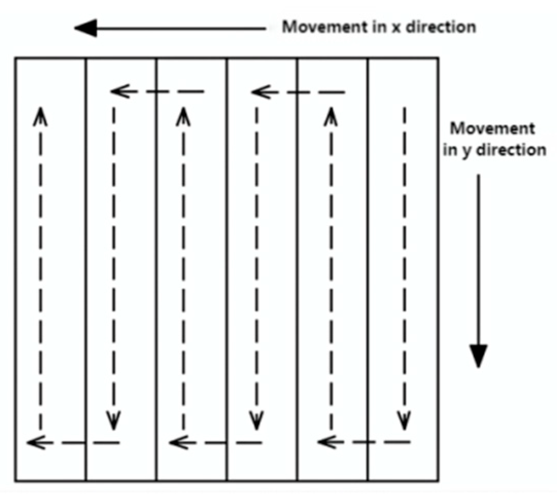
The laser rangefinder sensor uses a blue semiconductor laser with a wavelength of 405 nm, and the laser beam is 32 mm wide. The effective measurement range is ±23 mm, and the resolution is 0.05 mm. The measurement range of the instrument can reach 300 mm × 300 mm, and the effective width of a single scan is 30 mm. The schematic diagram of the laser beam movement route during measurement is shown in Figure 4.

2.3. Road Profile Characteristics and Anti-Slip Indexes

The texture of road surfaces at different scales directly affects the contact characteristics between tire treads and the road surface, thereby impacting the road’s anti-skid performance, noise levels, ride comfort, and tire wear. Based on the wavelength of the texture, the International Association for Road Surface Technology (The Permanent International Association of Road Congress, abbreviated as PIARC) [19] categorizes road surface textures into four types: unevenness, macro-texture, macroscopic texture, and microscopic texture. The classification indicators of pavement texture and their impact on different pavement performance are shown in

Table 1. Wavelengths of pavement surface texture.

Classify	Micro-Texture	Macro-Texture	Coarse Texture	Irregularity Degree
wavelength (mm)	<0.5	0.5~50	50~500	500
amplitude (mm)	<0.5	0.1~20	0.1~50	— —
The performance of the impact	adhesion	drainability	driving comfort	driving comfort

— — stands for no data range.

.

Micro-texture of the road surface refers to wavelengths and amplitudes both less than 0.5 mm, primarily manifesting as the undulating characteristics of the exposed aggregate surface. This is related to the mineral composition of the aggregates, lithology, and the source of the aggregates (natural or synthetic). It ensures basic friction under low-speed dry road conditions and rapidly breaks down the thin water film on wet roads, increasing the contact area between the tire and the road surface, thereby enhancing anti-skid performance [29]. Macro-texture refers to wavelengths ranging from 0.5 to 50 mm and amplitudes from 0.1 to 20 mm, mainly characterized by the undulating properties between aggregates on the road surface. This is associated with the geometric shape, gradation composition, and construction techniques of the aggregates. Under high-speed wet road conditions, it provides rapid drainage channels, reducing the likelihood of water skidding and ensuring driving safety [22]. Coarse texture refers to wavelengths ranging from 50 to 500 mm and amplitudes from 0.1 to 50 mm, primarily resulting from irregular surfaces caused by non-standard operations during construction. These can easily lead to localized water accumulation, increase tire rolling resistance, and generate significant road noise. During construction, efforts should be made to avoid the formation of coarse texture. Unevenness refers to wavelengths greater than 500 mm, mainly caused by serious quality issues during asphalt paving or significant damage and uneven settlement during use. This can result in large areas of water accumulation on the road surface, causing severe noise and affecting passenger comfort. The formation of unevenness should be avoided.

The macro- and micro-texture of the road surface is an important factor affecting the anti-slip performance of the road surface. Different levels of macro- and micro-texture will directly affect the contact characteristics of the road surface between the tire and the water. However, at present, the simulation techniques of micro-texture are limited. This paper will mainly focus on the influence of different macro-texture levels on the anti-slip performance of the road surface.

3. Test Methods

3.1. Material Preparation

3.1.1. Road Surface Materials

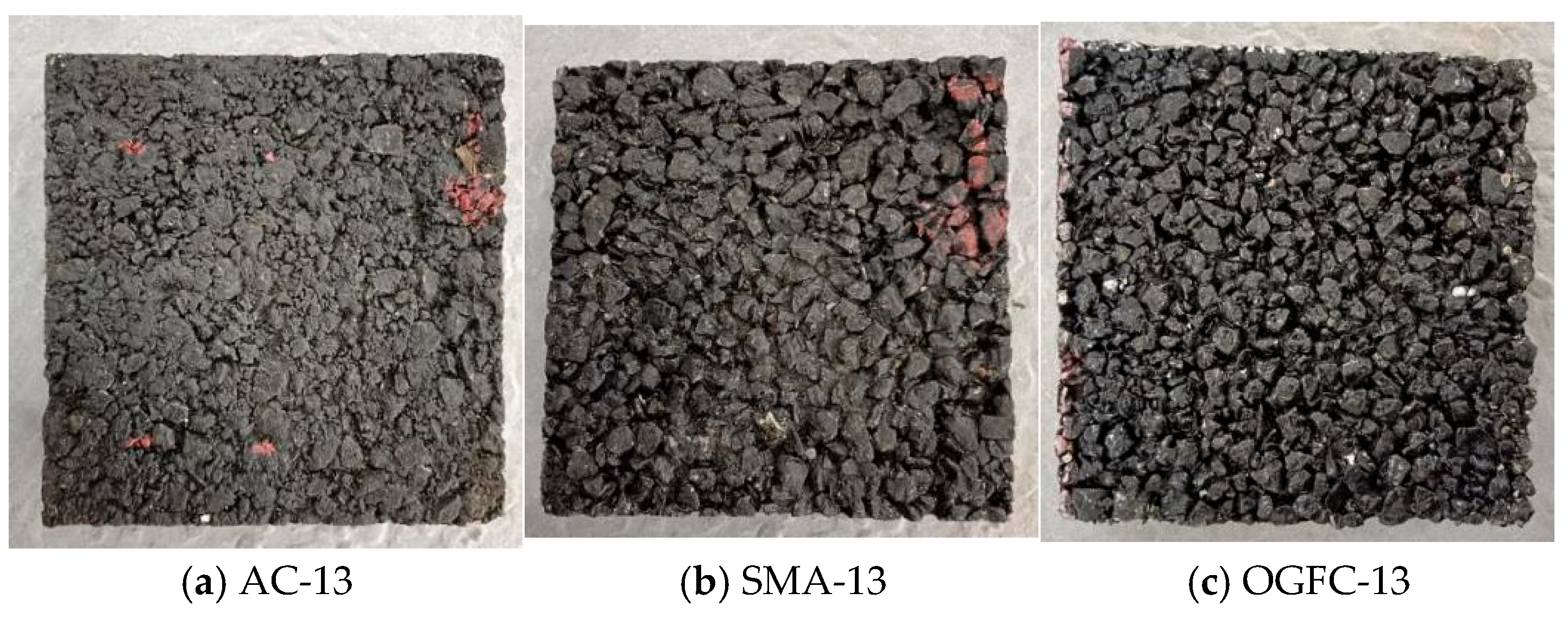
To investigate the impact of texture on anti-skid performance for different pavement types, this paper selects commonly used continuous dense-graded mix AC-13, traditional skeleton-compacted asphalt macadam SMA-13, and open-graded asphalt mix OGFC-13 as research subjects. Three different asphalt mixtures were formed into five rutting specimens, each measuring 300 mm in length, 300 mm in width, and 50 mm in height, according to their gradation design and optimal asphalt content, as shown in Figure 5.

The gradation composition is shown in Figure 6.

3.1.2. Measurement of Pavement Texture Index

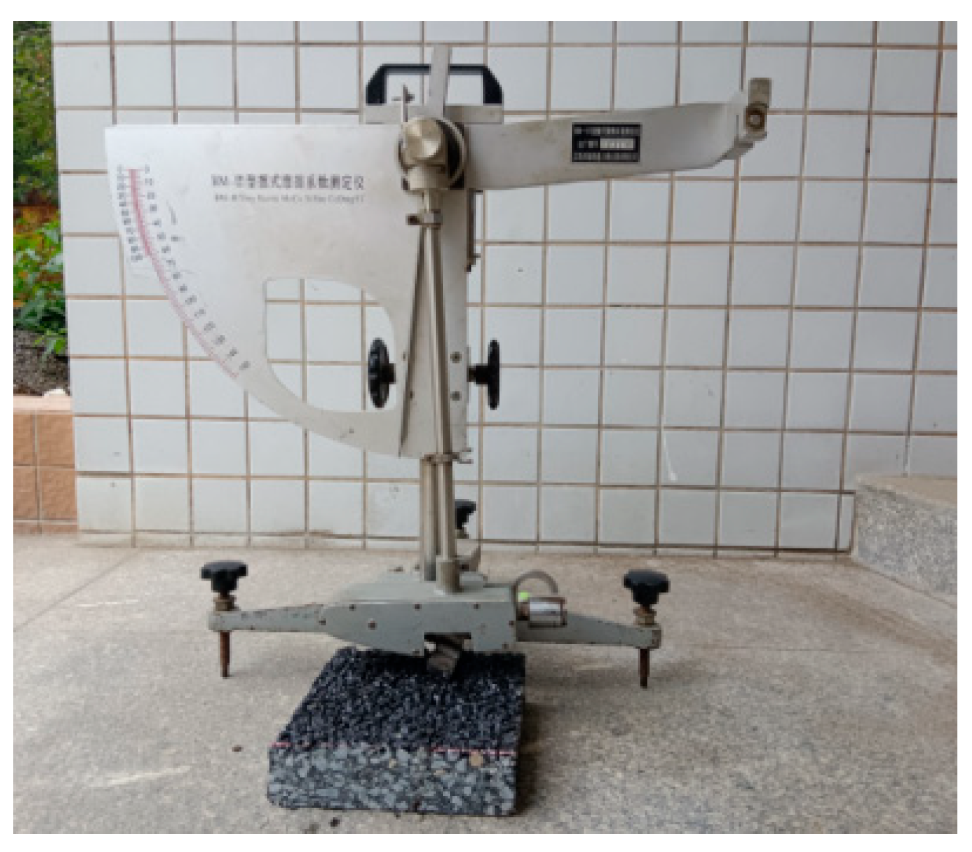
First, the oscillating friction coefficient tester was used to test the rutting specimens of three types of asphalt mixtures that had already been formed, as shown in Figure 7. The average value of five tests was taken as the oscillation value for each pavement, and the test results are presented in

Table 2. Asphalt pavement BPN values.

Type of Pavement	Bump Value (BPN)
	1	2	3	4	5	Average Value
AC-13	57.6	60.1	58.8	59.2	59.8	59.1
SMA-13	67.6	69.2	68.3	67.4	68.5	68.2
OGFC-13	74.4	73.6	75.2	73.5	75.3	74.4

. The ranking of the oscillation values for each asphalt pavement is as follows: O GF C-13 > SMA-13 > AC-13.

Secondly, the point cloud data measured by MATLAB (Version R2021a) are used to calculate the average cross-sectional construction depth (Mean Texture Depth, MTD) of each rutting plate, and the calculation formula is as follows:

$$\mathrm{M}\mathrm{P}\mathrm{D}={\displaystyle \frac{{\mathrm{h}}_{\mathrm{m}\mathrm{a}\mathrm{x}1}+{\mathrm{h}}_{\mathrm{m}\mathrm{a}\mathrm{x}2}}{2}}-\overline{\mathrm{h}}={\displaystyle \frac{{\sum }_{\mathrm{i}=1}^{\mathrm{n}}(\frac{{\mathrm{h}}_{\mathrm{m}\mathrm{a}\mathrm{x}1}+{\mathrm{h}}_{\mathrm{m}\mathrm{a}\mathrm{x}2}}{2}-{\mathrm{h}}_{\mathrm{i}})}{\mathrm{n}}}$$

(3)

The average value of the five tests is taken as the MTD of each pavement, and the test results are shown in

Table 3. MDP of asphalt pavement.

Type of Pavement	Average Construction Depth (mm)
	1	2	3	4	5	Average Value
AC-13	1.03	0.98	1.06	0.96	1.08	1.022
SMA-13	1.88	1.86	1.85	1.83	1.77	1.838
OGFC-13	2.08	2.12	2.06	2.05	2.03	2.068

. The average section construction depth of each asphalt pavement is ranked as follows: OGFC-13 > SMA-13 > AC-13.

3.2. Simulation Model

3.2.1. Tire Modeling

The focus of this study is the influence of different road surfaces on water accumulation and water sliding. Considering the use of computing resources, tire modeling is simplified to a certain extent under the condition of ensuring the accuracy of the road surface model, and tire modeling is selected with representative tire size and tread pattern.

Referring to existing research [30,31,32], the current weight range of passenger vehicles is approximately 1800–2300 KG. Additionally, 205/55 R16 tires are chosen by a significant portion of passenger vehicles. Therefore, this experiment selected this model of tire as the research subject. The factors ultimately determining the water skid resistance of the tire model also include tire load, tire pressure, tread pattern, and tread depth. Specifically, the tire load is 40 KN (400 KG), the tire pressure is 0.23 MPA, and the tread depth is 8 mm.

Tires are classified into two major categories based on their structural design: bias-ply tires and radial tires. Bias-ply tires have cross-laid cords that run diagonally across the carcass, with the crown and sidewalls sharing the same layer of fabric. They offer high strength, moderate elasticity, and strong load-bearing capacity, but they suffer from stress concentration, making sidewall deformation more likely to propagate to the tread, leading to unstable contact area and poor grip. Radial tires have nearly parallel cords arranged in the cross-section, with small cord angles, a rational structure, excellent wear resistance, low rolling resistance, good adhesion and cushioning properties, high load-bearing capacity, and are less prone to puncture. Currently, the main type of tire used in the market is the radial tire [33].

Meridian tires are made from a composite of rubber and cord skeleton materials, with a complex structure. Rubber is an ultra-elastic material with super elasticity and viscoelasticity, capable of absorbing impact energy, and is wear-resistant and impact-resistant. It mainly includes tread rubber, crown rubber, and carcass rubber. The cord skeleton consists of two layers of cords and one layer of skeleton, as shown in Figure 8.

Tire rubber materials are made from processed natural rubber, with a complex molecular structure that combines superelasticity and viscoelasticity, exhibiting highly nonlinear deformation under force. Scholars both domestically and internationally have studied their mechanical properties using various methods, establishing models such as Mooney-Rivlin, Neo-Hookean, and Yeoh, which are included in the Abaqus material library. Among these, the Neo-Hookean model is simple and versatile, suitable for simulating mechanical behavior at small strains, making it ideal for complex finite element models involving tire-soil-road coupling, with high computational accuracy [34,35,36]. Therefore, this paper adopts the Neo-Hookean model to describe the superelastic characteristics of tire rubber materials, with its strain energy relationship given by:

$$\mathrm{U}={\mathrm{C}}_{10}({\mathrm{I}}_1-3)+{\displaystyle \frac{1}{{\mathrm{D}}_1(\mathrm{J}-1)}}$$

(4)

In the formula, U is the strain potential energy, C10 is the material constant, I1 is the first invariant, J is volume change, and D1 is the material parameter, which represents the incompressibility of the material.

The Neo–Hookean model parameters and material density [37], obtained from the relevant test results of rubber materials, are shown in

Table 4. Parameters of rubber materials for meridian tires.

Material Parameter	Neo–Hookean Model
	C10 (MPa)	D1 (MPa-1)	ρ (g/cm3)
green tread	0.835	0.024	1.12
Cap gum	0.869	0.04	1.12
Body glue	1.0	0.02	1.15

.

At the same time, because rubber materials have the characteristics of super elasticity and viscoelasticity, it is necessary to choose an appropriate viscoelastic constitutive model to simulate tire rubber materials. The constitutive model selected in this paper is the genetic gene model [35], and its constitutive model relationship is shown in Equation (5) [37].

$$\mathsf{\sigma }={\int }_0^{1}2\mathrm{G}(\mathrm{t}-\mathsf{\tau }){\displaystyle \frac{\mathrm{d}\mathrm{e}}{\mathrm{d}\mathsf{\tau }}}\mathrm{d}\mathsf{\tau }+\mathrm{I}{\int }_0^1\mathrm{K}(\mathrm{t}-\mathsf{\tau }){\displaystyle \frac{\mathrm{d}\mathsf{\Delta }}{\mathrm{d}\mathsf{\tau }}}\mathrm{d}\mathsf{\tau }$$

(5)

In the equation, σ is the Cauchy stress, G (t) is the shear relaxation kernel function, K (t) is the volume relaxation kernel function, e is the shear strain, Δ is the volume deformation strain, t is a certain time, and τ is the past time.

The viscoelastic behavior of rubber materials is described using a generalized Maxwell model, in which the time-dependent shear and bulk relaxation moduli, G(t) and K(t), are expressed as Prony series expansions (Equations (6) and (7)). This formulation is widely used in commercial finite element software such as Abaqus (Version 2021^®) to represent linear viscoelasticity in the time domain [37].

$$\mathrm{G}(\mathrm{t})={\mathrm{G}}_{\mathrm{\infty }}+\sum _{\mathrm{i}=1}^{{\mathrm{n}}_{\mathrm{G}}}{\mathrm{G}}_{\mathrm{i}}\exp (-{\displaystyle \frac{\mathrm{t}}{{\mathsf{\tau }}_{\mathrm{i}}^{\mathrm{G}}}})$$

(6)

$$\mathrm{K}(\mathrm{t})={\mathrm{K}}_{\mathrm{\infty }}+\sum _{\mathrm{i}=1}^{{\mathrm{n}}_{\mathrm{K}}}{\mathrm{K}}_{\mathrm{i}}\exp (-{\displaystyle \frac{\mathrm{t}}{{\mathsf{\tau }}_{\mathrm{i}}^{\mathrm{K}}}})$$

(7)

In the formula, ${\mathrm{G}}_{\mathrm{\infty }}{,\mathrm{G}}_{\mathrm{i}}$, are the shear ${\mathrm{K}}_{\mathrm{\infty }}$ and modulus ${\mathrm{K}}_{\mathrm{i}}$, and ${\mathsf{\tau }}_{\mathrm{i}}^{\mathrm{G}}$ and ${\mathsf{\tau }}_{\mathrm{i}}^{\mathrm{K}}$ are the volume modulus and the relaxation time of each component.

The viscoelastic constitutive model parameters [35] are obtained by referring to the relevant literature, as shown in

Table 5. Prony series parameters.

Rubber Material	Prony Series Parameters
	${\overline{{\mathbf{g}}_1}}^{\mathbf{p}}$	${\overline{{\mathbf{k}}_1}}^{\mathbf{p}}$	${\mathbf{T}}_1$
Tread, crown, body glue	0.3	0	0.1

.

To simulate rubber-tire cord composite materials, this paper adopts the reinforcement (Rebar) element from Abaqus, where the material orientation rotates with deformation, better reflecting actual working conditions. Compared to anisotropic membrane elements, this approach can avoid computational errors under large strains. The Rebar element requires defining the cross-sectional area, spacing, angle, modulus, Poisson’s ratio, and density [36], as shown in

Table 6. Parameters of carcass material for radial tires.

Material Parameter	Cross-Sectional Area (mm2)	GAP (mm)	Angle (°)	Modulus (105 MPa)	Poisson Ratio	Density (g/cm3)
Tire cord 1	0.212	1.16	70	1.722	0.3	5.9
Tension wire 2	0.212	1.16	110	1.722	0.3	5.9
Tension wire skeleton	0.421	1.0	0	9.87	0.3	1.5

.

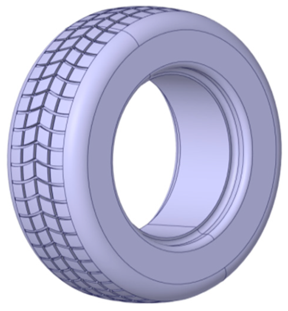
The tire pattern and model are shown in Figure 9.

3.2.2. Road Surface Modeling

The laser scanning instrument mentioned above was used to collect the THREE-DIMENSIONAL data of the road surface, and the texture information of AC-13, SMA-13 and OGFC-13 road surfaces was obtained. The following is the complete process of the road surface THREE-DIMENSIONAL model construction:

• Surface point cloud information processing. Using a laser texture measuring instrument to linearly measure the surface of each asphalt mixture rut, we obtained elevation information of the road surface texture with a data point interval of 0.05 mm, which is the point cloud data. The point cloud data were then exported as a.csv file; before reconstruction, preprocessing of the point cloud data is required. First, due to alternating measurement paths, the order of adjacent scan segments must be adjusted to ensure consistent point cloud sorting. Second, because the laser beam may produce multiple reflections in the texture gaps, some elevation information cannot be collected, and the system assigns these values to the scan limit value, forming “out-of-limit points”. To ensure reconstruction accuracy, the number of out-of-limit points should be controlled within 5% of the total number of points; if exceeded, a re-scan is necessary. For identified out-of-limit points, linear interpolation using adjacent valid points is used for correction. The above processing is implemented through MATLAB, ultimately obtaining high-precision point cloud data. Taking the AC-13 pavement as an example, its point cloud imported into CAD appears as shown in Figure 10a.
• Reverse reconstruction of pavement point cloud information.

During the process of reconstructing the road surface in reverse, point cloud data are processed using reverse modeling techniques to construct a simulation model that closely matches the actual road surface structure. This paper employs Geomagic Studio software (Version 12^®) developed by Geomagic to achieve the three-dimensional reconstruction of point cloud data. The software supports the automatic conversion of point clouds into polygonal meshes, mesh simplification, and polygon-to-NURBS surface conversion, and can be exported in various standard formats such as STL, IGES, STEP, and CAD files.

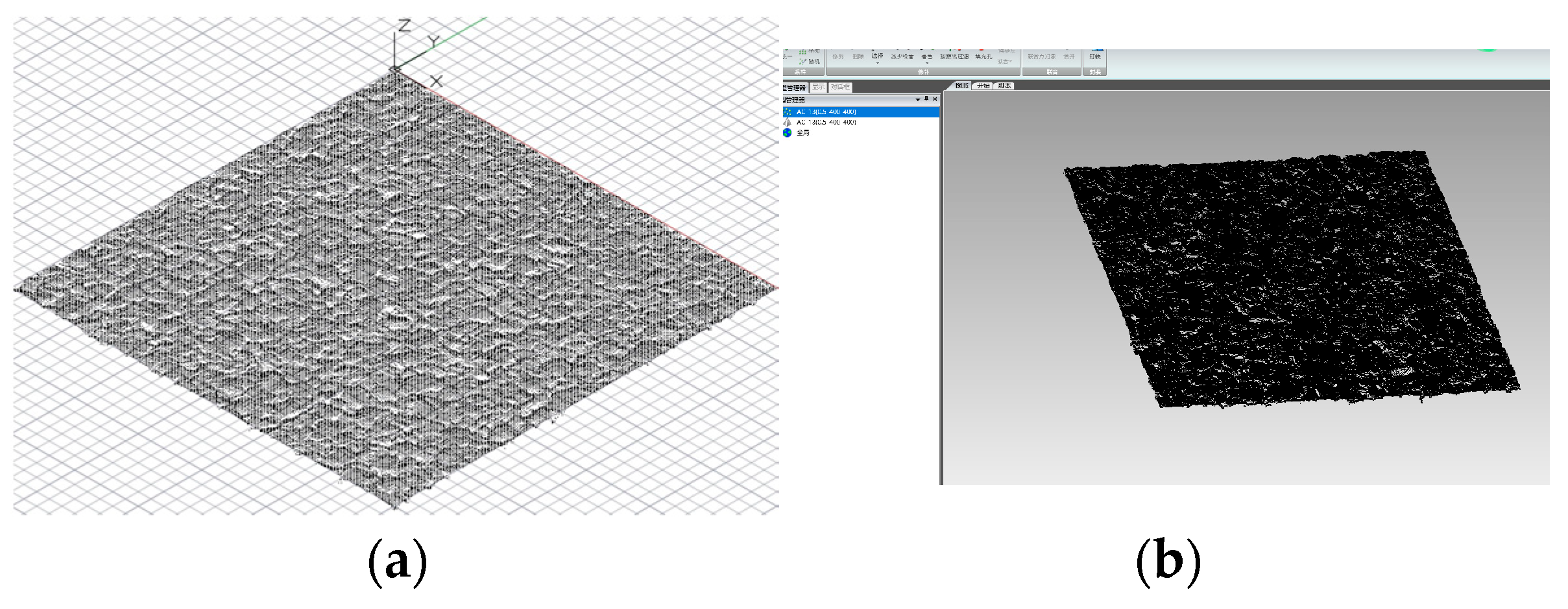
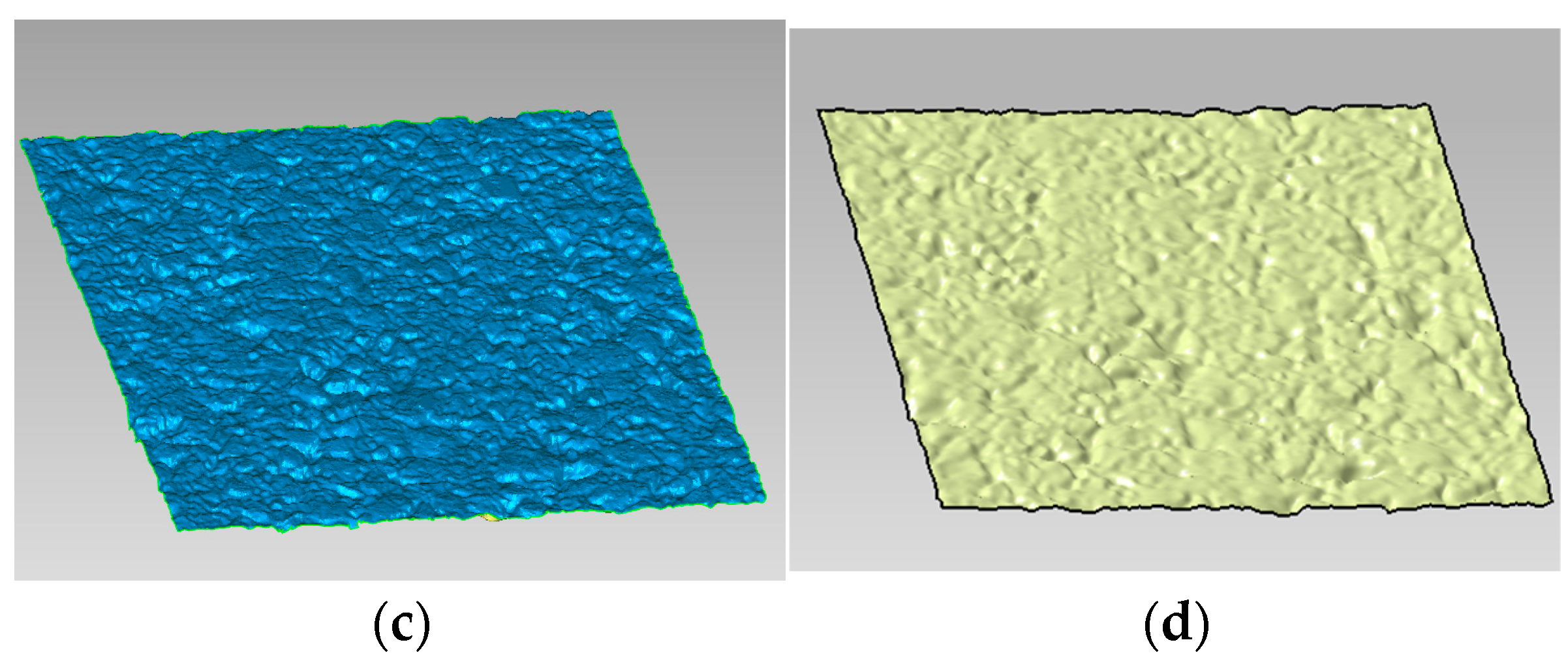
Taking the AC-13 pavement as an example, the reconstruction process is divided into three stages: point cloud processing, polygon processing and accurate surface fitting.

(1)

Point cloud processing

After the collected point cloud data are imported into Geomagic Studio, coloring processing is required to improve visibility, and then the point cloud is encapsulated into an initial polygonal mesh, as shown in Figure 10b.

(2)

Polygon processing

Automatic triangulation is used to generate polygonal surface patches for the road. Due to the complex texture of the road surface, sharp points or error points may occur during the triangulation process. The “Mesh Doctor” tool is used to remove abnormal patches, and a curvature-based local filling method is employed to repair defects, ensuring mesh continuity and obtaining a complete triangular mesh model, as shown in Figure 10c.

(3)

Exact surface fitting

After obtaining the mesh model, the geometry profile is constructed and NURBS surface fitting is performed by editing the contour lines and surface segments to make fine adjustments. To achieve accurate surface reconstruction from laser-scanned point cloud data, the NURBS (Non-Uniform Rational B-Spline) method was employed in this study. NURBS offers strong geometric flexibility and smoothness, making it particularly suitable for modeling complex and irregular pavement textures. Compared with simple polygonal or spline fitting techniques, NURBS provides better continuity and control over local surface features, which is essential for preserving the macroscopic texture relevant to hydroplaning analysis. The mathematical expressions for NURBS curves and surfaces are given in Equations (8) and (9), respectively:

$$\mathrm{p}(\mathrm{u})={\displaystyle \frac{{\sum }_{\mathrm{i}=0}^{\mathrm{n}}{\mathsf{\omega }}_{\mathrm{i}}{\mathrm{N}}_{\mathrm{i},\mathrm{k}}(\mathrm{u}){\mathrm{p}}_{\mathrm{i}}}{{\sum }_{\mathrm{i}=0}^{\mathrm{n}}{\mathsf{\omega }}_{\mathrm{i}}{\mathrm{N}}_{\mathrm{i},\mathrm{k}}(\mathrm{u})}},0\le \mathrm{u}\le 1$$

(8)

In the formula, ωi (I = 0, 1…, n) is the weight coefficient; Ni and K(μ) are B-spline basis functions; Pi is the control point. By increasing the number of iterations, NURBS curves can be extended to NURBS surfaces, resulting in the expression of NURBS surfaces [35,37]:

$$\mathrm{p}(\mathrm{u})={\displaystyle \frac{{\sum }_{\mathrm{i}=0}^{\mathrm{m}}{\sum }_{\mathrm{j}=0}^{\mathrm{n}}{\mathrm{N}}_{\mathrm{i},\mathrm{k}}(\mathrm{u}){\mathrm{N}}_{\mathrm{j},\mathrm{l}}(\mathrm{v}){\mathsf{\omega }}_{\mathrm{i}\mathrm{j}}{\mathrm{p}}_{\mathrm{i}\mathrm{j}}}{{\sum }_{\mathrm{i}=0}^{\mathrm{m}}{\sum }_{\mathrm{j}=0}^{\mathrm{n}}{\mathrm{N}}_{\mathrm{i},\mathrm{k}}(\mathrm{u}){\mathrm{N}}_{\mathrm{j},\mathrm{l}}(\mathrm{v}){\mathsf{\omega }}_{\mathrm{i}\mathrm{j}}}},\mathrm{u},\mathrm{v}\in [\mathrm{0,1}]$$

(9)

The NURBS fitting can obtain an accurate surface model with good geometric continuity and realize high-fidelity road reconstruction, as shown in Figure 10d.

3.

The meshing of the pavement model (Figure 11). In Geomagic Studio software, the reverse reconstructed pavement model is exported as an.iges file and imported into Hypermesh software for meshing. During the meshing process, considering that the quality of the mesh significantly affects the accuracy and convergence of simulation results, the pavement surface should be divided into quadrilateral elements as much as possible, with triangular elements used only at the sharp corners of the surface. A too dense mesh increases computational time costs, while a too sparse mesh affects result accuracy. Therefore, the side length of the pavement mesh is generally within the range of 2 mm to 4 mm.

3.2.3. Water Body Modeling

In the analysis of tire-fluid-road interaction, there are two models [38]: the water flow model and the tire rolling model, as shown in Figure 12. The water flow model simplifies calculations by setting the tire rotation speed and applying reverse translational velocities to the road surface and water flow, making it efficient and easy to converge, but unable to accurately simulate water flow patterns. The tire rolling model pre-sets a water film on the road surface, assigning rotational and translational speeds to the tires, which more realistically reflects the working state of the tires and water flow patterns, but has low computational efficiency and is prone to non-convergence. Studies have shown that the two models differ little when simulating mechanical indicators such as tire-road contact forces [23]. Given that this study focuses on the contact characteristics of tires and roads under water accumulation conditions, with non-water flow patterns being less critical, the more computationally efficient water flow model is selected.

In the tire-water-road coupling analysis, water flow is impacted by the high-speed rotation of tires, resulting in complex mechanical responses. Abaqus provides a variety of state equations to describe the behavior of water flow. In this paper, the MIE–GRUNEISEN state equation [35,36] is selected to describe the relationship between water flow density and pressure, with the basic form as follows:

$$\mathrm{P}={\mathrm{P}}_{\mathrm{H}}(1-{\displaystyle \frac{{\mathsf{\Gamma }}_0\mathsf{\eta }}{2}})+{\mathsf{\Gamma }}_0{\mathsf{\rho }}_0{\mathrm{E}}_{\mathrm{m}}$$

(10)

In the formula, P is the stress of the fluid; PH is the impact pressure; Γ0 is the material parameter; η = 1 − ρ₀/ρ, where ρ₀ is the initial density of the fluid, kg/m³; ρ is the density of the fluid after impact, kg/m³; Em is the specific internal energy of the fluid, PH is the impact pressure, and the specific relationship is shown in Formula (11):

$${\mathrm{P}}_{\mathrm{H}}={\displaystyle \frac{{\mathsf{\rho }}_0{\mathrm{c}}_0\mathsf{\eta }}{(1-\mathrm{s}\mathsf{\eta }{)}^2}}$$

(11)

In this formula, C₀ is the sound velocity of the fluid, m/s; s is the material constant, and the relationship between C₀ and s is shown in Formula (12).

$${\mathrm{U}}_{\mathrm{s}}={\mathrm{c}}_0+\mathrm{s}{\mathrm{U}}_{{\mathrm{p}}_{\mathsf{\nu }}}$$

(12)

In the formula, Up is the impact velocity, where Up refers to the motion velocity of the particle. By applying the law of conservation of energy to the above (9)–(11) formulas, the relationship between fluid stress and fluid density can be obtained as shown in Formula (13).

$$\mathrm{P}={\displaystyle \frac{{\mathsf{\rho }}_0{\mathrm{c}}_0\mathsf{\eta }}{(1-\mathrm{s}\mathsf{\eta }{)}^2}}(1-{\displaystyle \frac{{\mathsf{\Gamma }}_0\mathsf{\eta }}{2}})+{\mathsf{\Gamma }}_0\mathsf{\eta }{\mathrm{E}}_{\mathrm{m}}$$

(13)

In this study, the parameters in the MIE–GRUNEISEN state equation were determined [39] by referring to the relevant literature, as shown in

Table 7. Parameters of the MIE–GRUNEISEN state equation.

Material	ρ0 (kg/m3)	c0 (m/s)	s	Γ0
water	1000	1484	1.979	0.11

.

The water film finite element model uses a water-air composite model, with dimensions of 300 mm × 300 mm × 100 mm. It includes a lower water film area (height varies with the thickness of the water film) and an upper air area (ensuring space for water flow). The modeling steps are as follows: first, meshing is performed in Hypermesh using Eulerian elements EC3D8R; second, the tire-water flow coupling region is refined, with a total of 62,209 nodes and 56,687 elements; finally, the mesh is imported into Abaqus (Figure 13).

3.2.4. Tire-Fluid-Road Coupling Contact Modeling

The contact between tires and the road surface is a nonlinear problem, making modeling complex. Abaqus software provides two algorithms for general contact and contact pairs. The general contact algorithm has a simple definition and imposes fewer restrictions on the contact surfaces; the contact pair algorithm is suitable for complex contact behaviors, offering high computational efficiency but requiring strict adherence to contact surfaces. This paper selects the contact pair algorithm to define contact behavior, which includes point-to-surface and surface-to-surface contact types, both of which are solved through discretization.

Point-to-surface contact is established by searching for the main surface element from the surface node to create contact elements (Figure 14a). The calculation is simple and converges easily, but it tends to produce penetration phenomena, which do not fully match the actual tire-road contact, leading to lower accuracy. Face-to-face contact involves finding adjacent surface patches from nodes and using the N2S method to determine the main surface patch, establishing multiple contact elements (Figure 14b). This effectively avoids penetration and aligns with the actual tire-road contact, resulting in higher accuracy. Therefore, this paper adopts face-to-face contact.

The main surface and the secondary surface should be defined for face-to-face contact. The selection criteria of the main surface are as follows: the surface with a large stiffness difference is selected; the surface with similar stiffness is selected when the mesh is coarse. In this paper, the road surface contact surface is taken as the main surface, and the tire contact surface is taken as the secondary surface.

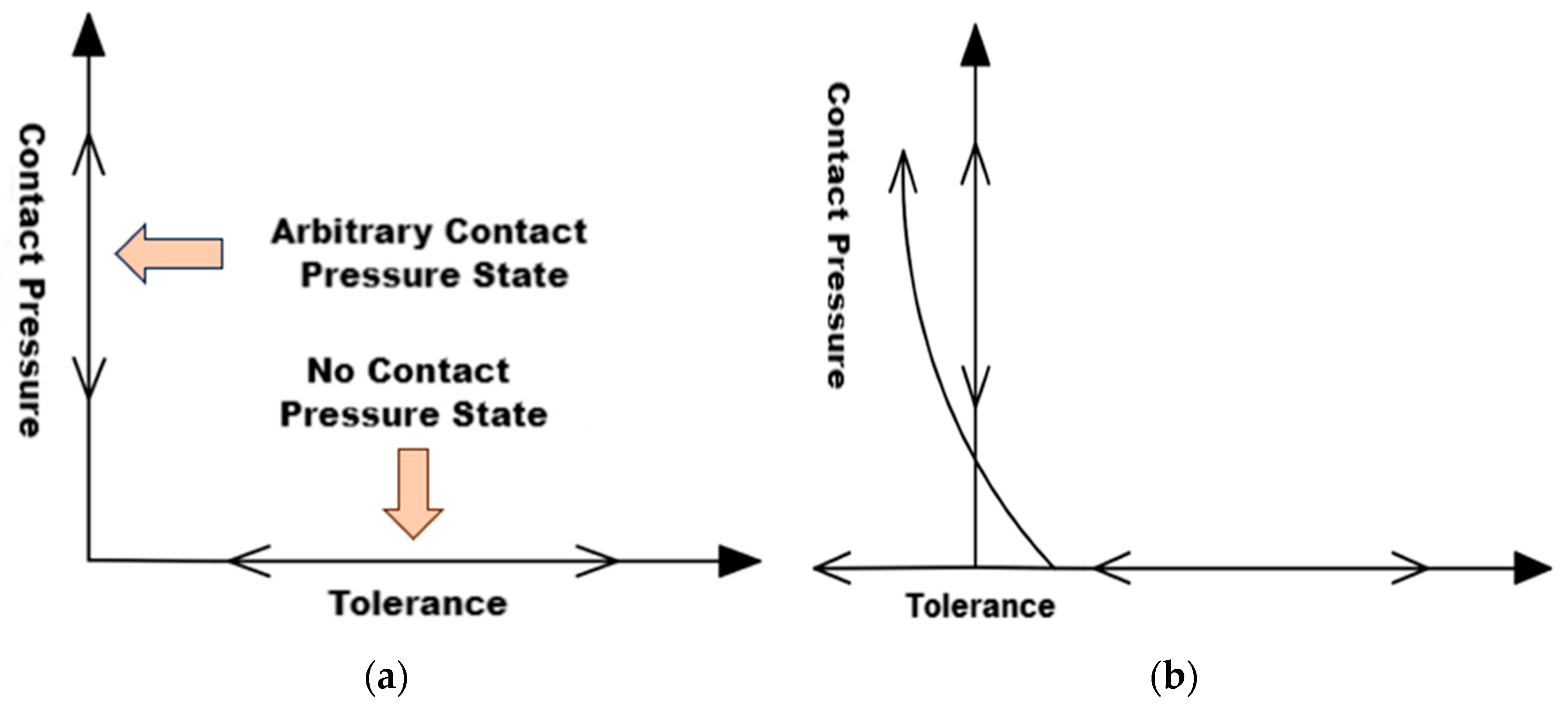
Contact properties include normal and tangential attributes. Normal contact is divided into hard and soft contact. Hard contact does not allow penetration, with zero clearance allowing infinite pressure (Figure 15a); soft contact (exponential, linear, tabular models) allows penetration, with the amount depending on parameters (Figure 15b). Hard contact better represents the actual tire-road contact, hence the hard contact model is selected.

Tangential contact includes exponential friction, Coulomb friction and custom model. The Coulomb friction model is simple to calculate and has good convergence, which can be divided into isotropic and anisotropic. In this paper, the isotropic Coulomb friction model is selected to define the tangential contact attribute.

The tangential contact properties mainly include the exponential friction model, Coulomb friction model, and custom models. Among these, the Coulomb friction model can describe the running state in the tangential direction of the contact model, which includes two types: isotropic and anisotropic. Compared with other friction models, the Coulomb friction model is characterized by simple calculations and good convergence. Therefore, this paper selects the isotropic Coulomb friction model to define the tangential contact properties between tires and the road surface.

To accurately simulate the tire-road contact behavior, the tire boundary conditions are set as follows: release the translational degrees of freedom in the Z direction to simulate vertical loads; constrain the translational and rotational degrees of freedom in the X and Y directions to ensure that the tire only moves vertically. The road surface boundary conditions constrain all six degrees of freedom to simulate a fixed road surface. In static analysis, a tire load along the Z-axis is applied, with a friction coefficient set to 0 to simplify initial contact calculations. In steady-state analysis, the friction coefficient can be adjusted to reflect actual friction behavior. These settings aim to balance computational accuracy and efficiency, realistically representing the contact state between the tire and the road surface

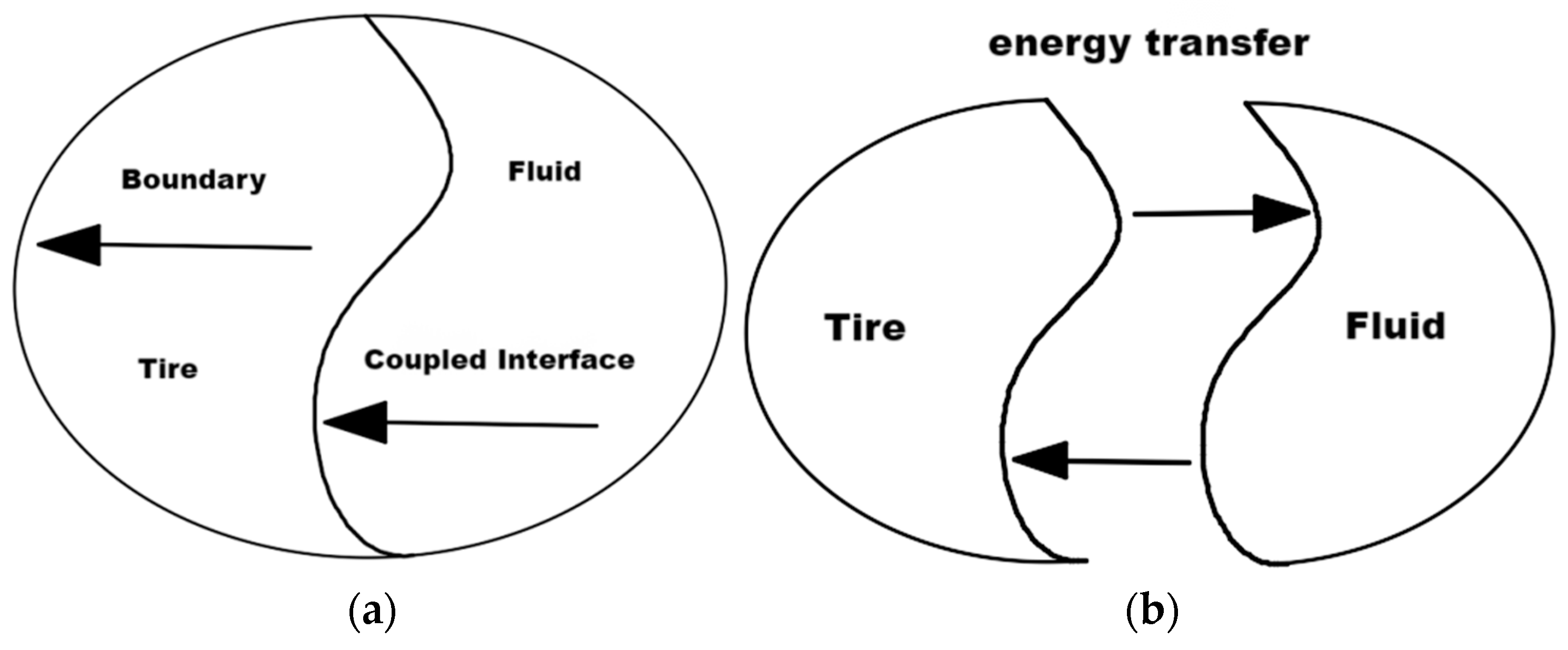
In the tire-water-road coupling modeling, it is necessary to select the type of fluid-solid coupling. Abaqus provides two methods: strong coupling and weak coupling [35]. In strong coupling (Figure 16a), the tire and water share a unified control equation, and coupling interface parameters are obtained through discrete solving, ensuring continuous and smooth physical quantities at the interface. In weak coupling (Figure 16b), the tire dynamics and fluid control equations are solved separately, and boundary parameters are iteratively transferred to make the coupling interface parameters consistent. Due to significant differences in mesh size and element properties between the tire and fluid, strong coupling is difficult to converge, while weak coupling can effectively address these property differences, ensuring computational accuracy and stability. Therefore, this paper adopts weak coupling for the fluid-solid coupling interface.

To simulate the interaction between tire-road and tire-water-road coupling, the boundary conditions are set as follows: the tire is released from translational freedom in the Z direction but constrained in translational and rotational freedom in the X and Y directions to simulate vertical loads; in explicit calculations for coupled analysis, the rotational freedom in the Y direction of the tire is released while other constraints remain, and the tire’s rotational speed is set. The road surface constraint is applied to all degrees of freedom except translational movement in the X direction, with the translational speed in the X direction set to simulate relative motion. The water film model sets the translational speed and outflow speed to reflect the dynamics of water flow. In static analysis, a tire load is applied along the Z-axis with a friction coefficient of 0; in steady-state analysis, the friction coefficient, road surface translational speed, and tire rotational speed can be adjusted to analyze the coupled effects under different conditions. These settings balance computational accuracy and efficiency, realistically reflecting the interaction between tire-road and tire-water-road.

4. Result Analysis

4.1. Water Flow Imprint and Vertical Contact Variation Law

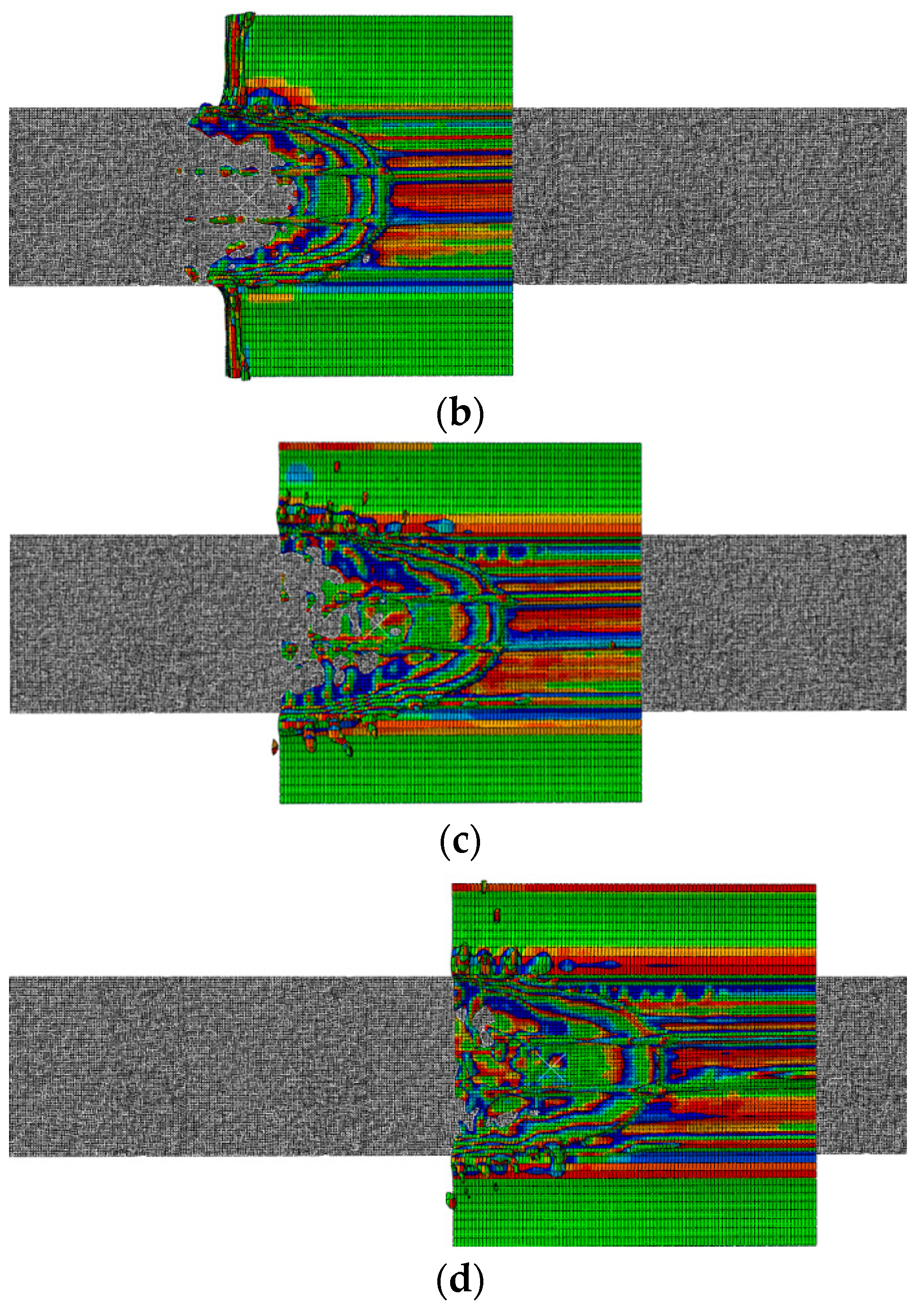
In the tire-road water coupling model, the internal inflation pressure of the tire is set to 0.23 Mpa, the tire load is 4000 N, the tire speed is 120 km/h, and the water film thickness is 8 mm. Taking the SMA-13 pavement as an example, after simulation analysis, the motion traces of water impact on the tire can be output in the post-processing module view interface of Abaqus software for different analysis times, as shown in the figure. The vertical contact force variation pattern between the tire and the road during the analysis time of 0.03 s is shown in Figure 17.

As shown in Figure 17a, at the analysis time of 4.0075 s, water flow on the road surface has already come into contact with the tires. The water flow, compressed by the high-speed rolling of the tires, flows around the tires and partially splashes out. Due to the presence of tire grooves, some of the water also enters these grooves. As shown in Figure 17b, at the analysis time of 4.0105 s, the area where the water flow from the road surface contacts the tires further expands. The tires can almost completely drain the water, leaving only some water in the grooves. As shown in Figure 17c, at the analysis time of 4.0150 s, under the effect of high-speed rolling, the water flow from the road surface cannot be completely drained around the tires and will invade the bottom of the tires, increasing the lifting force on the tires, thus continuously reducing the contact area between the tires and the road surface. As shown in Figure 17d, at the analysis time of 4.0210 s, the tires fully enter the water flow area on the road surface, and the area invaded by water continues to increase, causing the tires to no longer make contact with the road surface, resulting in a skidding phenomenon.

4.2. Distribution of Dynamic Water Pressure on Different Road Surfaces

Considering that the supporting force provided by the road surface is the source of friction between the tire and the road surface, when the dynamic water pressure caused by the water accumulation is greater than or equal to the load of the tire, it can be considered that the tire and the road surface have produced water sliding. Figure 18 shows the variation of dynamic water pressure on three kinds of roads at different speeds when driving on the water-accumulated road surface.

As can be seen from the figure, the common characteristics of dynamic water pressure distribution on different road surfaces are as follows:

The dynamic water pressure is positively correlated with the thickness of the water and the driving speed. At the same speed, the dynamic water pressure increases with the increase in water thickness, and the increasing rate also gradually increases; at the same water film thickness, the dynamic water pressure increases with the increase in vehicle speed.

When the water film thickness is in the range of 2–8 mm, the dynamic water pressure increases more rapidly with increasing vehicle speed and water film thickness. When the water film thickness is in the range of 8–20 mm, the dynamic water pressure increases more slowly with increasing vehicle speed and water film thickness. The two patterns change at a boundary of 8 mm for the water film thickness. This is because when the water film thickness is less than 8 mm, the longitudinal tread grooves of the tire have an 8 mm drainage channel, which allows water to be discharged to both sides as it flows over the tire, resulting in a relatively slower increase in the lifting force of the water on the tire. As the water film thickness gradually exceeds 8 mm, the longitudinal tread grooves are filled with water, preventing the tire from quickly discharging water from both sides, causing the water to accumulate on the tire sidewall and leading to a sharp increase in dynamic water pressure. When the water film thickness continues to increase, although the accumulation of water increases, the change in dynamic water pressure is not significant. According to the theory derived from the literature [40], the actual formula for calculating dynamic water pressure is as follows:

$$\mathrm{P}=\mathsf{\rho }{\displaystyle \frac{{\mathrm{V}}^2}{2}}$$

(14)

In the formula, p is the maximum pressure of the tire facing the water, Pa; v is the relative velocity of the tire and water film, m/s; p is the water flow density, kg/m.

From this, it can be seen that the only variable in the formula is speed, meaning the dynamic water pressure is solely related to the speed of travel [41]. However, during the conversion from pressure to dynamic water pressure, factors such as the tire contact area and the contact area between the water film and the tire must also be considered. Similarly, when converting, the impact of the road surface on dynamic water pressure must also be taken into account. Under equal conditions, the size of the dynamic water pressure is OGFC < SMA < AC for paved roads. On paved roads, vehicles can achieve the critical dynamic water pressure threshold for skidding at higher speeds and with thicker water films, providing better anti-skid performance and safety margin. In contrast, while SMA pavement shows good anti-skid performance in terms of indicators, its actual simulation results in poor anti-skid effects. The SMA pavement does not significantly alleviate dynamic water pressure, and in some cases, it may not differ much from AC pavement.

4.3. Changes in Critical Water Sliding Velocity

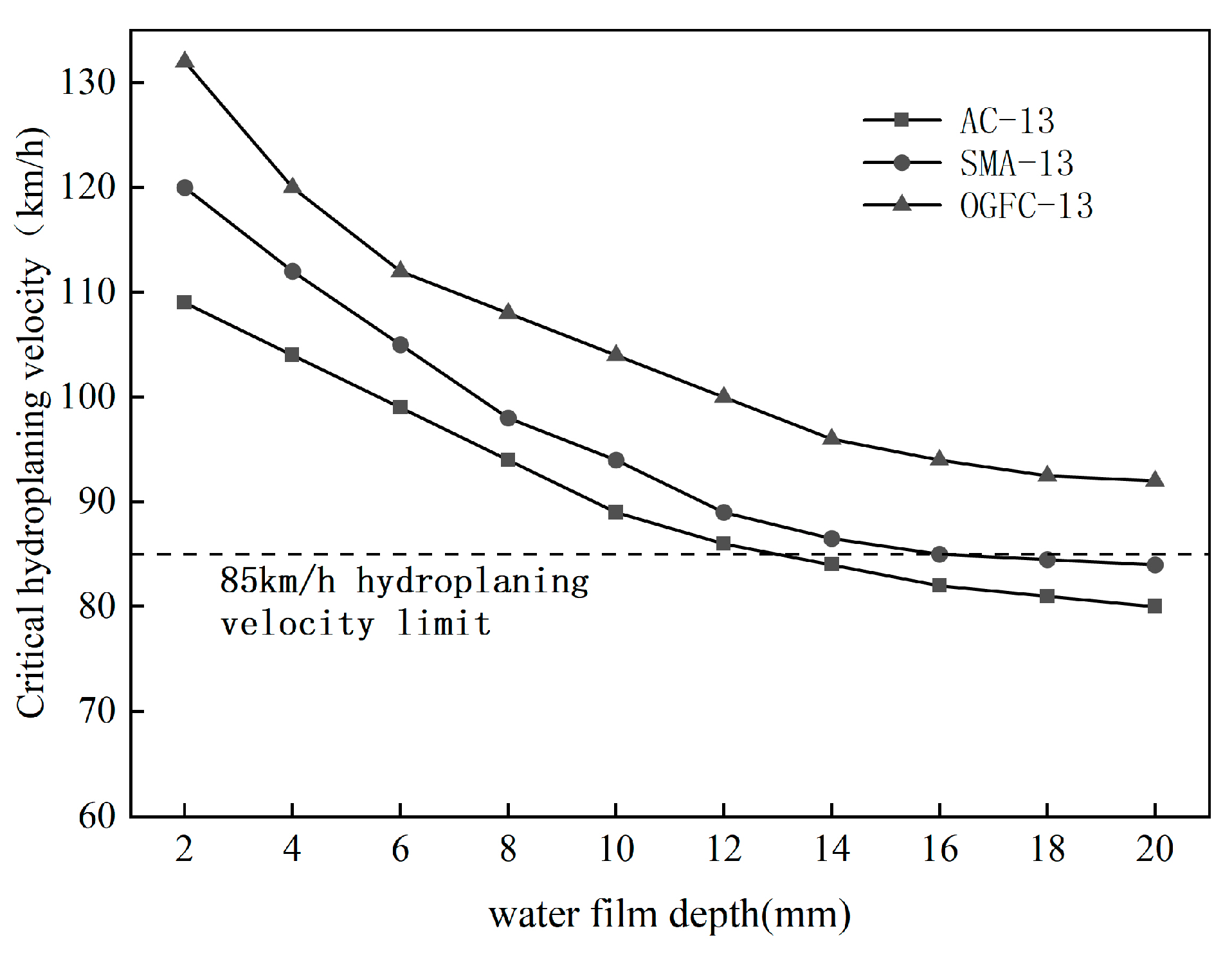
The critical water sliding speed on the road surface can be considered to be the speed that causes the dynamic water pressure to be equal to the tire in a certain water film thickness, in which case the road surface and the tire just slip. The boundary water sliding speed on different roads is shown in Figure 19.

As can be seen from the figure above, the overall trend of the critical water slip velocity under the three kinds of road surfaces is to decrease with the increase of water film thickness. The reduction rate of the critical water slip velocity is faster in the range of 2–10 mm, and the reduction trend of the critical water slip velocity becomes slower after 10 mm.

In addition, there are the following rules:

• Under the same water film thickness conditions, the critical water skid speed for different road surfaces is OGFC > SMA > AC, indicating that OGFC pavement has better anti-skid performance compared to other pavements. However, the SMA pavement does not show a significant improvement in anti-skid performance compared to the AC pavement, especially when the water film thickness is relatively high. The water skid curves of both are very close, which does not correspond to the actual measured anti-skid indicators.
• Referring to the critical water speed marked in the figure, the critical water film thickness corresponding to the three kinds of road surface is 16 mm for the SMA road surface and 13 mm for the AC road surface, while the OGFC road surface can pass through the road surface with a 20 mm water film thickness at the speed of 85 km/h under the simulated condition.
• As analyzed above, the critical water skid speed begins to decrease sharply when the water film thickness reaches around 8 mm. Essentially, the 8 mm longitudinal tread pattern on tires can no longer promptly drain surface water, leading to a sharp reduction in the critical water skid speed. To ensure that more vehicles have sufficient safe driving speeds, it is necessary to establish lower safe driving speeds for rainy weather. To guarantee the safety of most vehicles, it is recommended to set a safe water film thickness of 4 to 5 mm.

4.4. Influence of Road Surface Texture Uniformity on Anti-Slip Performance

Although it can be seen from the measurement results of the road anti-slip index in the previous text that the swing value and MTD of the SMA-13 and the OGFC-13 roads are not much different, the swing value and MTD of the two roads differ by 8.3% and 6.7% on average, but the maximum dynamic water pressure in the same situation differs by 13.8%.

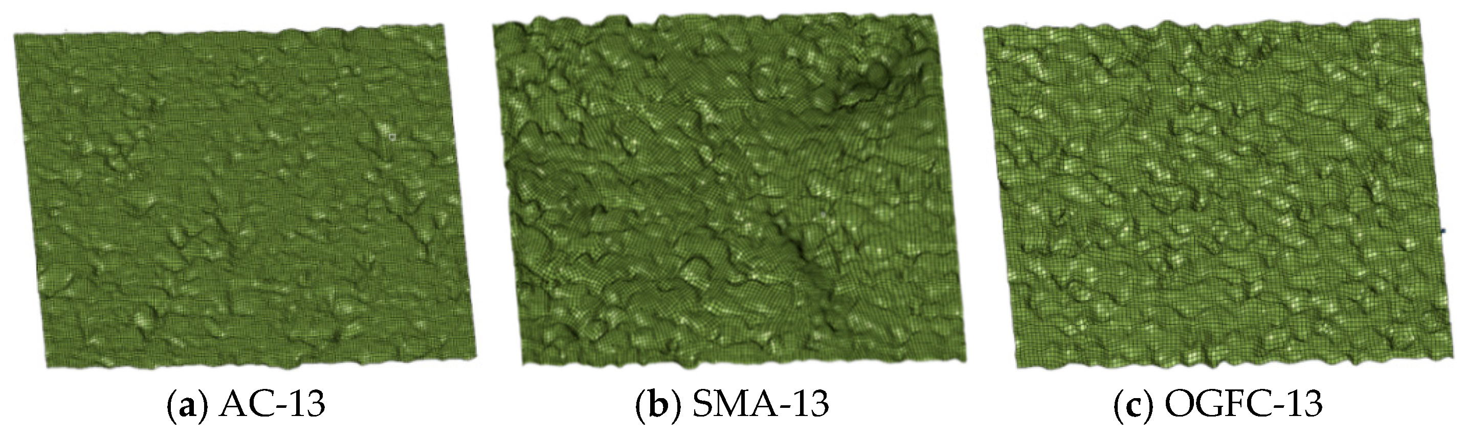
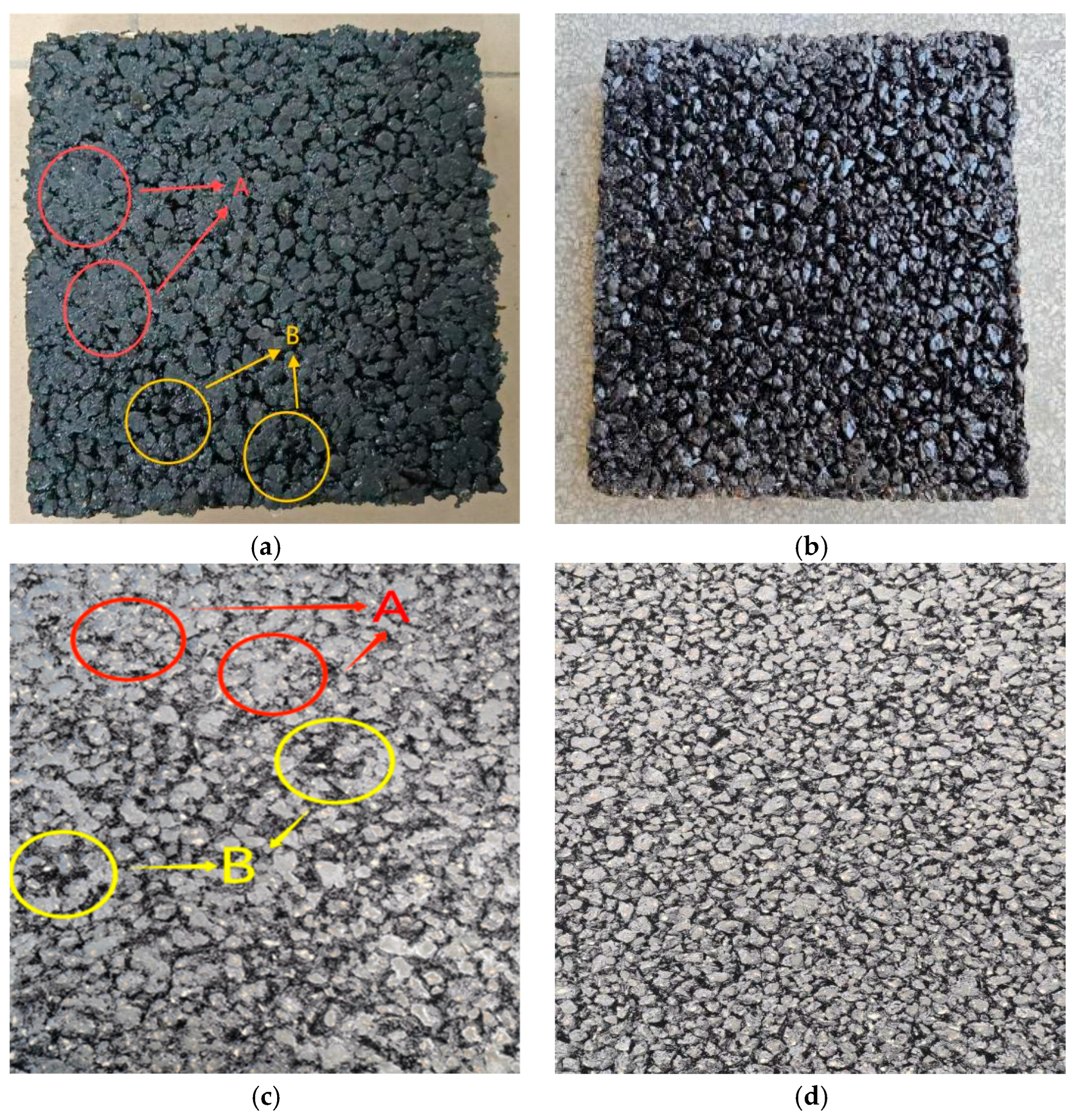
Through the re-analysis of the actual road surface, it is evident that in multiple SMA rutting plates, there are areas with uneven construction distribution as shown in the Figure 20(a) and (c). At location A marked on the map, due to the close packing of stone materials and the accumulation of asphalt paste, the structure has become shallower or even disappeared. In contrast, at location B marked in Figure 20(a) and (c), due to the lack of stone materials, the structure has become deeper and larger. The interaction between these two factors results in an average construction depth that is not small, yet the overall uniformity of the SMA pavement structure is poor. In comparison, as shown in Figure 20 (b) and (d) the construction uniformity of the OGFC is better, with a more even distribution across the surface. The unevenness in construction leads to significant differences in actual anti-skid performance despite similar values for slip resistance and MTD between the two different gradations.

Research shows that after the initial paving of [42] and SMA, due to the presence of a large amount of asphalt and mineral powder in the SMA mix, it is prone to issues such as oil spots, leading to uneven pavement structure. Additionally, excessive asphalt coating prevents the aggregate from coming into contact with tires, resulting in poorer anti-skid performance. After a certain period of operation, the anti-skid performance of SMA pavements improves due to the redistribution of the asphalt and exposure of the aggregate.

It can be seen that MDP and swing friction value cannot completely evaluate the anti-slip condition of the road surface, and the evaluation of the road surface texture should also consider the uniform distribution of the road surface texture.

5. Analysis of Uniformity Index of Pavement Texture

In order to comprehensively evaluate the influence of pavement texture on anti-slip, The Anti-Slip Comprehensive Texture Index (ACTI) is proposed.

To comprehensively evaluate the uniformity of pavement texture and its influence on skid resistance under wet conditions, the Anti-Slip Comprehensive Texture Index (ACTI) is introduced. This model integrates three core components—benchmark compliance, asymmetrically weighted variation, and gain-controlled spatial compensation—into a unified framework. Specifically, the ACTI is formulated as:

$$\mathrm{A}\mathrm{C}\mathrm{T}\mathrm{I}=\underset{\mathrm{Benchmark} \mathrm{Compliance}}{\underbrace{\sqrt{{\displaystyle \frac{\mathsf{\mu }}{\mathrm{T}}}}}}\cdot \underset{\mathrm{Asymmetric} \mathrm{Weighting}}{\underbrace{\exp (-{\displaystyle \frac{\sum {\mathrm{w}}_{\mathrm{i}}\cdot |{\mathrm{M}\mathrm{D}\mathrm{P}}_{\mathrm{i}}-\mathsf{\mu }|}{\mathsf{\mu }}})}}\cdot \underset{\mathrm{Gain} \mathrm{Control}}{\underbrace{(1+{\displaystyle \frac{{\mathrm{N}}_{\mathrm{high}}}{\mathrm{n}}}\cdot {\displaystyle \frac{1}{1+{\mathsf{\sigma }}_{\mathrm{high}}}})}}$$

(15)

Here, µ denotes the mean texture depth, and T = 0.5 mm serves as the benchmark threshold. The weight wi is designed to penalize insufficient texture more heavily than it rewards excessive texture, and is defined as:

$${\mathrm{w}}_{\mathrm{i}}=\left\{\begin{array}{c}2.0\cdot {\displaystyle \frac{\mathrm{T}-{\mathrm{M}\mathrm{D}\mathrm{P}}_{\mathrm{i}}}{\mathrm{T}}},{\mathrm{M}\mathrm{D}\mathrm{P}}_{\mathrm{i}}<T\\ 0.5\cdot {\displaystyle \frac{{\mathrm{M}\mathrm{D}\mathrm{P}}_{\mathrm{i}}-\mathrm{T}}{\mathsf{\mu }}},{\mathrm{M}\mathrm{D}\mathrm{P}}_{\mathrm{i}}\ge T\end{array}\right.$$

(16)

The gain control term enhances the ACTI value when numerous high-texture subregions exist with low internal variability. In this context, N_high represents the count of subregions where ${\mathrm{M}\mathrm{D}\mathrm{P}}_{\mathrm{i}} \ge \mathrm{T} + 0.05 \mathrm{mm}$, and σ_high denotes the standard deviation of these subregions. The total number of measurement sub-regions, n, is typically set to nine.

This formulation ensures sensitivity to both global texture levels and local deviations. Benchmark compliance prevents overvaluation based solely on high averages; asymmetric weighting highlights texture deficiencies; and gain control enhances robustness against sporadic high readings. Consequently, the ACTI is particularly suitable for evaluating different asphalt mixtures, such as AC, SMA, and OGFC, on a unified scale.

The key parameters and their engineering significance are summarized as follows:

T (reference texture depth) can be adjusted based on requirements and minimum texture height requirements for different regions.

µ (Mean texture depth): µ = $\mathsf{\mu }={\displaystyle \frac{1}{\mathrm{n}}}{\sum }_{\mathrm{i}=1}^{\mathrm{n}}{\mathrm{M}\mathrm{D}\mathrm{P}}_{\mathrm{i}}$. It indicates the average texture condition.

w_i (Asymmetric weighting function): Defined above. It penalizes low texture and rewards high texture.

N_high (Count of high-texture subregions): ${\mathrm{M}\mathrm{D}\mathrm{P}}_{\mathrm{i}} \ge \mathrm{T} + 0.05 \mathrm{mm}$. It identifies effective anti-skid texture points.

σ_high (Standard deviation of high-texture zones): $\sqrt{{\displaystyle \frac{1}{{\mathrm{N}}_{\mathrm{high}}}}{\sum }_{\mathrm{i}\in \mathrm{high}}({\mathrm{MDP}}_{\mathrm{i}}-{\mathsf{\mu }}_{\mathrm{high}}{)}^2}$. It evaluates the uniformity of high-texture contributions.

n (Total number of measurement subregions): Defined by the sampling grid (e.g., n = 9). It reflects the resolution of surface measurements.

The article provides a classification standard and engineering interpretation based on a construction depth of 0.5 mmACTI, as shown in

Table 8. ACTI Grading Standards and Engineering Interpretation.

ACTI Level	ACTI Range	Description
Excellent	ACTI ≥ 1.5	Texture distribution is uniform and overall exceeds the standard; high texture areas are densely distributed.
Good	1.0 ≤ ACTI < 1.5	The mean meets the standard; high texture areas effectively compensate for local fluctuations.
Marginal	0.7 ≤ ACTI < 1.0	The mean is critical; texture is unevenly distributed with many low texture areas.
Poor	ACTI < 0.7	The mean does not meet the standard or low texture areas are concentrated.

.

Then, the rutting plate was divided into nine parts at a distance of 100 mm, and the MTD of each sub-area was calculated. Finally, the ACTI results were obtained as shown in

Table 9. ACTI values of different road surfaces.

	OGFC-13		SMA-13		AC-13
Sample	MDP (mm)	ACTI	MDP (mm)	ACTI	MDP (mm)	ACTI
1	2.08	1.57	1.98	1.12	1.03	0.88
2	2.12	1.61	1.96	1.1	0.98	0.85
3	2.06	1.7	1.95	1.09	1.06	0.91
4	2.05	1.56	1.93	1.07	0.96	0.84
5	2.03	1.57	1.87	1.03	1.08	0.93
Mean	2.068	1.602	1.938	1.082	1.022	0.882

.

As can be seen from the table, in the ACTI coefficient, OGFC > SMA > AC, among which, although the pendulum friction values and the average structural depth of OGFC and SMA pavements are not much different (the average difference is 6%), the ACTI is very different (40%). Compared with the AC pavement, the pendulum friction value of the SMA pavement (difference of 15%) and the average structural depth (80%) are very different, but the ACTI coefficient is smaller (15%), which basically corresponds to the anti-skid performance of the AC pavement and the SMA pavement in the simulation. Therefore, in general, ACTI effectively considers the unevenness of the pavement structure, thereby evaluating the anti-skid condition of the pavement.

6. Conclusions

This study employed Abaqus software with Coupled Eulerian–Lagrangian (CEL) technology to simulate tire hydroplaning on laser-scanned road surfaces, focusing on the influence of pavement texture on anti-skid performance. The investigation analyzed three asphalt mixtures—AC-13, SMA-13, and OGFC-13—under varying water film thicknesses (2–20 mm) and vehicle speeds (up to 120 km/h). The key findings are summarized as follows:

Superior Anti-Skid Performance of OGFC-13: The OGFC-13 pavement exhibited the best anti-skid performance, followed by SMA-13, with AC-13 showing the poorest resistance to hydroplaning. This ranking aligns with the pavements’ ability to mitigate dynamic water pressure, with OGFC-13 maintaining effective drainage even at higher water film thicknesses and vehicle speeds.

Critical Role of Tread Depth: The tire tread depth (set at 8 mm) significantly influenced the hydroplaning behavior. A sharp increase in dynamic water pressure and a corresponding decrease in critical hydroplaning speed were observed when the water film thickness exceeded 8 mm, indicating the limit of the tire’s drainage capacity.

Impact of Texture Uniformity: Despite similar traditional anti-skid metrics (e.g., pendulum friction value and mean texture depth) for SMA-13 and OGFC-13, OGFC-13 demonstrated superior hydroplaning resistance due to its greater texture uniformity. This highlights the limitation of conventional metrics in capturing texture distribution effects.

Introduction of ACTI: A novel Anti-Slip Comprehensive Texture Index (ACTI) was proposed to evaluate pavement texture uniformity. The ACTI revealed significant differences in anti-skid performance, with OGFC-13 achieving a mean ACTI of 1.602 (excellent), SMA-13 at 1.082 (good), and AC-13 at 0.882 (marginal), better reflecting real-world hydroplaning outcomes compared to traditional metrics.

Practical Recommendations: To enhance safety under wet conditions, a maximum water film thickness of 5 mm and a vehicle speed limit of 80–85 km/h are recommended. Areas prone to water film thicknesses exceeding 5 mm should be treated to prevent hydroplaning risks.

These findings underscore the importance of pavement texture uniformity and tire tread depth in mitigating hydroplaning risks. Future research should explore tire performance variations, including tread depth degradation and pattern types, to further refine the safety guidelines for wet pavement conditions.