Article

A Forecasting Approach for Wholesale Market Agricultural Product Prices Based on Combined Residual Correction

Business School, Yangzhou University, Yangzhou 225127, China
*
Author to whom correspondence should be addressed.
Appl. Sci. 2025, 15(10), 5575; https://doi.org/10.3390/app15105575
Submission received: 2 April 2025 / Revised: 2 May 2025 / Accepted: 12 May 2025 / Published: 16 May 2025

Abstract

:
Wholesale market prices of agricultural products, being essential to the daily lives of consumers, are closely tied to living standards and the overall stability of the agricultural market. The use of a single model to predict nonlinear and dynamic agricultural price time series often results in low accuracy due to suboptimal use of available information. To address this issue, this paper proposes a combined residual correction-based prediction method. Initially, the sparrow search algorithm (SSA) is used to optimize the penalty factors and kernel parameters of support vector regression (SVR) and the input weights and hidden layer biases of the extreme learning machine (ELM), thereby improving the convergence rate and predictive accuracy of these models. Subsequently, the induced ordered weighted averaging (IOWA) operator is applied to determine the weight vectors for the SSA-SVR and SSA-ELM models, reducing the fluctuating prediction accuracies of individual models at different times. Finally, the residuals of the generalized regression neural network (GRNN) model are forecasted using a combined residual correction method that integrates SSA-SVR and SSA-ELM based on the IOWA operator, refining the GRNN’s forecast outcomes. An empirical analysis was performed by comparing the results of nine individual forecasting models on monthly pork prices in Beijing. The findings indicate that the SSA-SVR, SSA-GRNN, and SSA-ELM models outperformed the SVR, GRNN, and ELM models in terms of forecasting accuracy, respectively. This improvement is attributed to the parameter optimization of the SVR, GRNN, and ELM models through the SSA. The proposed model also showed superior forecasting accuracy compared to the nine individual models. The results confirm that the proposed model is an effective tool for predicting agricultural product prices and can be applied to forecast prices of other agricultural products with similar characteristics.

1. Introduction

Agricultural product prices, as an important component of the agricultural market in the modern economic system, are closely related to the vital interests of producers and operators, and even the quality of life of consumers [1]. A decrease in the prices of agricultural products in the wholesale market leads to a reduction in earnings for producers and traders, while an increase in these prices results in a higher cost of living for consumers. Moreover, frequent and significant price volatility can disrupt the stability of the market and impede the sustainable growth of the agricultural industry’s supply chain, ultimately harming the interests of producers, operators, and consumers [2,3]. Therefore, it is essential to carry out precise predictions regarding the trends of agricultural product price fluctuations.
Agricultural product prices in wholesale markets are affected by various external factors, including production costs, changes in supply and demand, climatic conditions, and government policies and interventions. The prices fluctuate rapidly and extensively, presenting nonlinear and non-smooth characteristics; therefore, accurately predicting agricultural prices is challenging. There are numerous models for the forecasting of agricultural commodity prices. Based on the number of models utilized, forecasting models can be classified as either single or combined models [4]. Models can be divided into two main types: statistical models and machine learning models. Statistical price forecasting models mainly comprise the trend extrapolation method, exponential smoothing method, regression forecasting method, and gray forecasting model [5,6]. While statistical models are characterized by the strong interpretability of the results, they have a limited capacity to handle complex nonlinear time-series data [6]. Due to their excellent self-learning and self-adaptive capabilities, machine learning models are widely applied in forecasting [7], and mainly include the backpropagation neural network (BPNN), general regression neural network (GRNN), support vector regression (SVR) [8], and extreme learning machine (ELM). However, these models are sometimes characterized by difficult parameter selection [9,10,11,12,13].
In order to enhance the predictive accuracy of individual models and to leverage their strengths while mitigating their weaknesses, the idea of composite forecasting was first proposed, which involves blending various individual forecasting techniques through a weighted average approach [14]. Ensemble forecasting models enhance the variety within predictive systems, allowing for the comprehensive retrieval of valuable insights from individual model forecasts and bolstering the stability of outcomes in unforeseen circumstances [15]. These ensemble models are broadly classified into three types. The initial type encompasses models that utilize data decomposition techniques [4]. Within the realm of intricate time-series forecasting, the strategy of decomposing and then integrating data is viewed as a potent approach to enhance predictive precision. The essence of this strategy lies in breaking down intricate time series into simpler, more manageable segments, which streamlines the forecasting model development process [3,16]. The second type of ensemble model is predicated on the assignment of weights, with the goal of allocating optimal weights to minimize the combined model’s predictive error, given that the weights are non-negative and normalized [17,18]. The primary methods for combining models in this category involve weighted averaging algorithms and techniques that minimize the aggregate sum of squared errors. The third type of ensemble forecasting model is founded on error correction principles. Given that errors in agricultural price forecasting are inevitable, employing an error correction strategy can mitigate these errors and, in turn, enhance the precision of the forecasted outcomes. The central tenet of this approach is to refine the current forecast by incorporating the immediate error [19].
Neural networks have robust capabilities for self-learning and adaptation, allowing them to approximate complex nonlinear functions with high accuracy and making them ideal for predicting agricultural prices. The BPNN, GRNN, and ELM are among the neural network models frequently employed in this domain [2,20]. Nevertheless, there is a dearth of models that focus on residual correction, especially those based on SVR and ELM. The performance of SVR is highly contingent on its penalty factors and kernel function parameters, which significantly affect the model’s convergence rate and accuracy [21]. Similarly, the randomly determined input weights and hidden layer biases of ELM can influence its learning efficiency and generalization ability [22,23]. In contrast to other algorithms, the sparrow search algorithm (SSA) distinguishes itself by its streamlined structure, minimal control parameters, precise solutions, and rapid convergence in optimization tasks [24,25]. This study utilizes SSA to optimize the penalty factors and kernel function parameters of SVR, as well as to fine-tune the input weights and hidden layer biases of ELM, thereby enhancing the predictive accuracy of both the SVR and ELM models. Traditional ensemble forecasting models assign uniform weight coefficients to the same single model at all time points within a sample interval. However, the accuracy of a single model can vary at different time points, revealing a limitation of the conventional ensemble forecasting approach. To overcome this, the induced ordered weighted averaging (IOWA) operator is introduced, which allocates weights to each individual forecasting model based on their accuracy at each specific time point within the sample interval.
To deal with the nonlinear, random, and multi-periodic intricacies that are inherently present in agricultural price time series, the aim of this research is to establish a forecasting approach that makes use of a combined residual correction strategy. At the beginning, the SSA is utilized to optimize the penalty factors and kernel function parameters of the SVR model, along with the input weights and hidden layer biases of the ELM model, with the intention of improving their predictive precision. Then, the IOWA operator is adopted to assign weights to each separate forecasting technique based on the accuracy of their fit at each particular time point within the sample period. This resolves the problem of the same weight coefficients being allotted to the same single forecasting method at every time point within the sample interval. Eventually, the residuals of the GRNN model are predicted by the optimal neural network residual correction method guided by the IOWA operator, resulting in an adjusted final forecast. To validate the effectiveness of the proposed model, it is applied to the dataset of the monthly pork price in Beijing, China, ranging from January 2009 to September 2024, with predictions for pork prices extending from October 2024 to December 2025. The establishment of a highly precise and practical pork price forecasting model will assist in uncovering the pattern of pork price variations. Furthermore, it will offer a significant decision-making foundation for producers and operators, as well as for the government to formulate appropriate regulatory policies and measures.
This paper is organized as follows: Section 2 conducts a review of the literature concerning price forecasting models, Section 3 elaborates on the construction of the proposed model, and Section 4 validates the model’s validity, makes a comparison with other forecasting models, and discusses the forecasting outcomes. Section 5 concludes the paper through an analysis.

2. Literature Review

Researchers have put forward a variety of approaches and models for predicting prices. Within this research, the methods for price prediction are bifurcated into two principal groups, individual forecasting models and ensemble forecasting models, differentiated by the quantity of models employed in the price prediction process.

2.1. Single Prediction Models

Individual price forecasting models can be classified into two general types: statistical and machine learning approaches. Statistical forecasting techniques mainly depend on the correlation between historical and future prices, presenting this relationship in a functional form. Common methods for price forecasting in this area comprise quadratic exponential smoothing, cubic exponential smoothing, the autoregressive integrated moving average (ARIMA) model, and grey model (GM) forecasting techniques [4,5,26,27,28].
These techniques project future price trends linearly using past price data, and their predictive accuracy tends to deteriorate with expanding time horizons. Given the inherent volatility and non-linearity of price series, traditional statistical forecasting methods struggle to capture these non-linear attributes [4], resulting in their limited effectiveness in producing reliable forecasts. Due to their robust non-linear adaptability and capacity to model the non-linear dynamics of price series effectively [29], machine learning models are gaining traction in price forecasting. Examples of such models include the BPNN, GRNN, ELM, SVM, recurrent neural network (RNN) [30], and long short-term memory (LSTM) [4,23]. Basically, machine learning models utilize a predictive framework to encompass the non-linear relationship between historical and future prices in a rather opaque “black box” way, instead of explicitly as a functional representation. While individual machine learning models can offer strong predictive performance, they are still subject to the influence of their own parameters [31,32,33,34].

2.2. Combined Prediction Models

The precision of individual predictive models is inherently prone to inaccuracies due to their inherent limitations, and they often fail to fully account for all aspects of the data. To address the issue of low predictive accuracy associated with single models, Bates and Granger introduced the idea of ensemble forecasting, which involves blending various single forecasting techniques, each with its own set of weights. By integrating the strengths of different standalone forecasting models that possess complementary traits, ensemble models can mitigate the drawbacks of individual models, which often exhibit significant errors in specific forecasting periods. This approach leads to the development of a highly precise forecasting model for prices [4,35]. In accordance with the theory of combination, ensemble forecasting models can be categorized into three main types.
(1) Ensemble forecasting models that utilize data decomposition techniques break down the price time series into several frequency-domain components. Individual models are then applied to predict each of these components separately. The forecasts from these individual components are subsequently aggregated to derive the overall price forecasting outcome [4]. An integrated approach has been put forward for forecasting vegetable prices over short, medium, and long horizons. The findings indicated that the proposed model is well-suited for predicting the prices of seasonal vegetables [3].
(2) Ensemble forecasting models that rely on weighted coefficients [4]. Given that the predictive performance of a single forecasting model can vary in strength or weakness at different times, these models can be merged by allocating them weight coefficients that sum up to 1. In a prior investigation, an ensemble forecasting model was constructed by assigning weights to the ensemble empirical modal decomposition (EEMD), radial basis neural network (RBFNN), and ARMIA models. The results indicated that the combined model performed better than each of the three individual models [17].
(3) Ensemble forecasting models that employ residual correction. This technique refines the forecasting outcomes by integrating the residual predictions from multiple models. By taking into account the full historical data, certain researchers have introduced the residual-driven support vector regression (SVR) model, which has seen widespread application in the forecasting of financial markets [19].

3. Model Construction

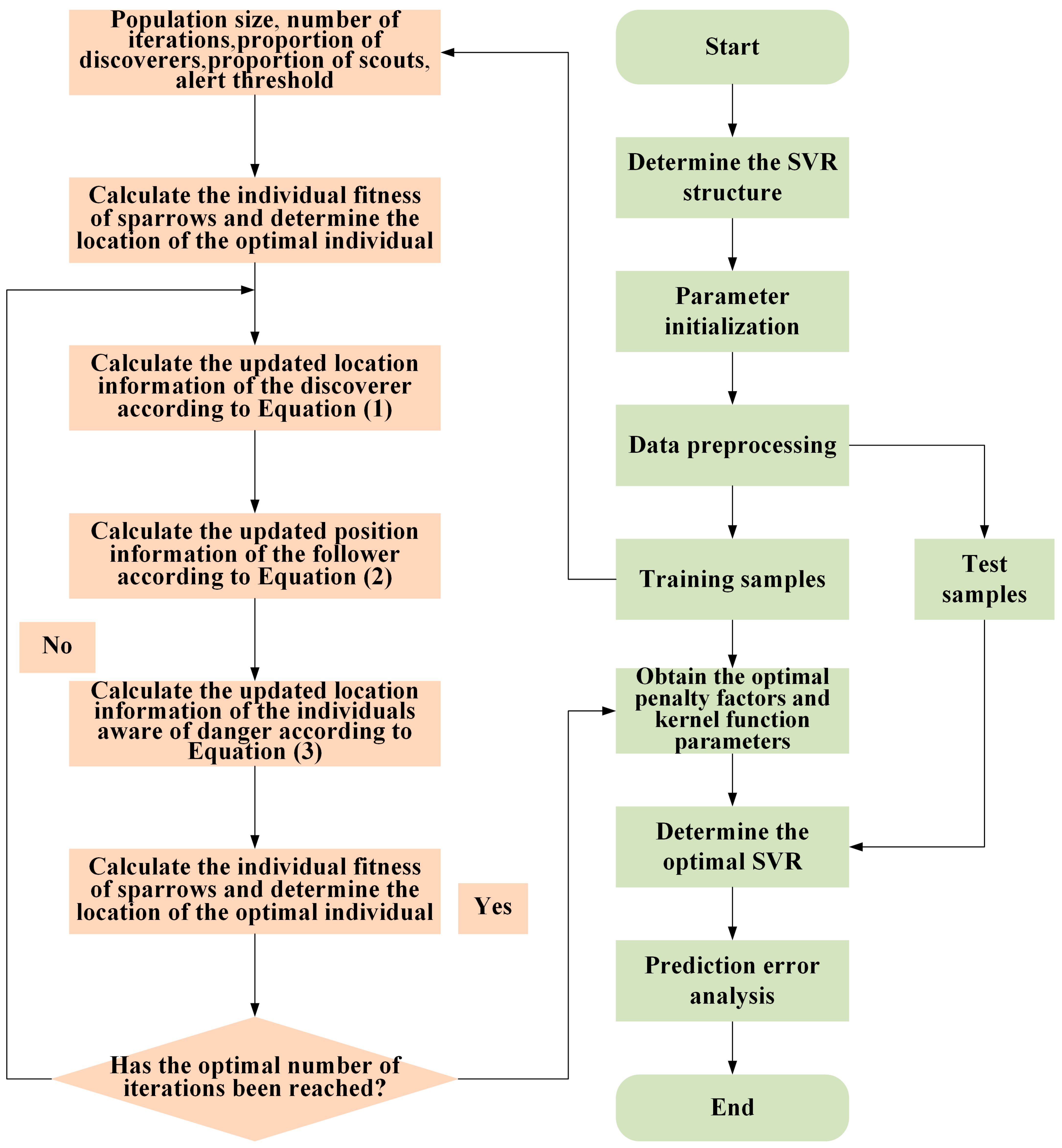
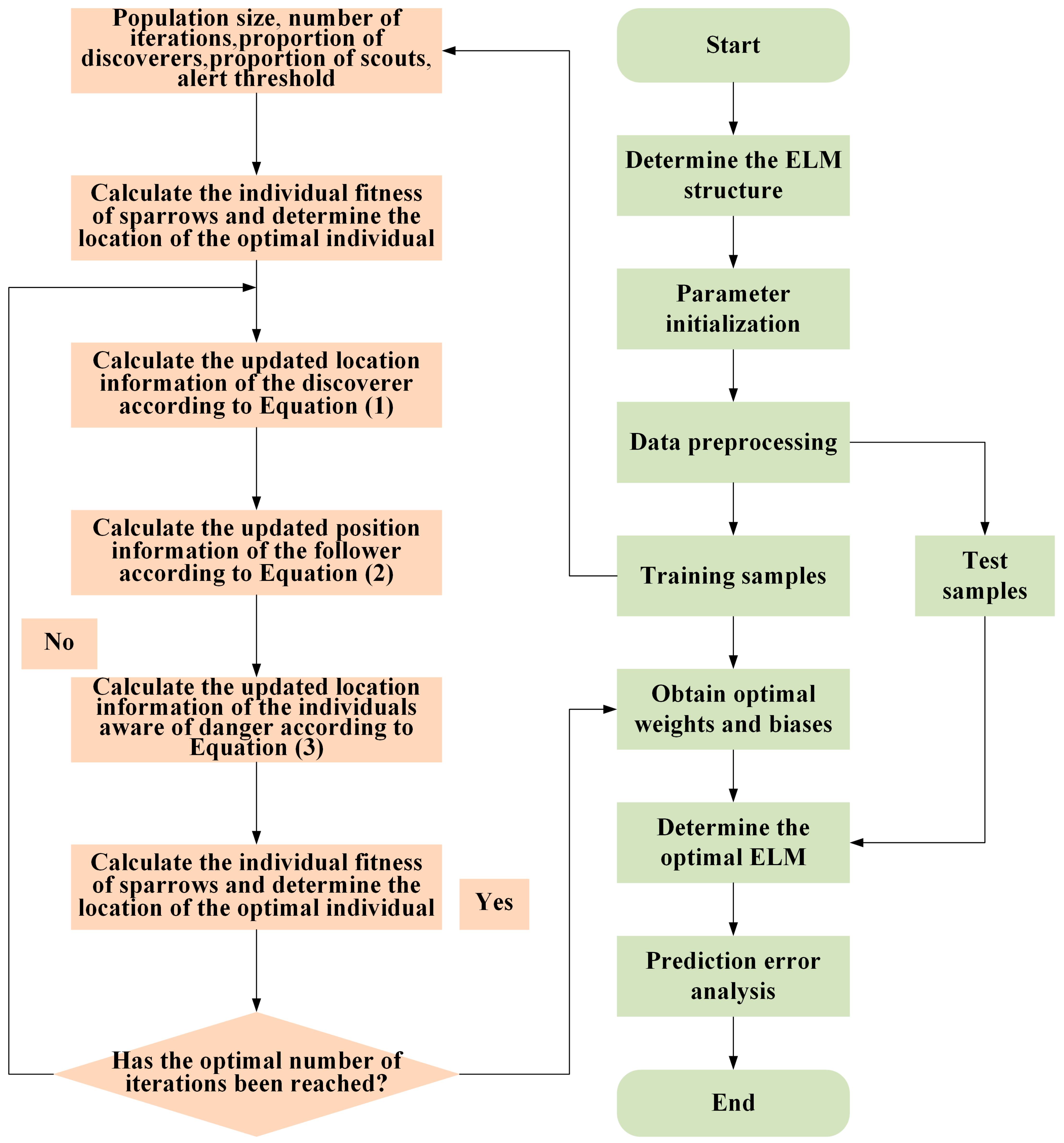
3.1. Optimized Prediction Model Construction

Optimization of the SVR and ELM Models Based on the SSA
Intelligent optimization algorithms are effective for parametric optimization and search tasks. The SSA, in particular, excels due to its simple design, few control parameters, high precision, and fast convergence, especially in complex optimizations [24,25]. It has been widely applied in fields like machine learning parameter optimization, engineering, and fault diagnosis [36,37]. Therefore, the SSA was chosen for optimizing the parameters of the SVR and ELM models. The optimization processes are illustrated in Figure 1 and Figure 2.
(1) Training and test set determination. The pork price data collected from Beijing serve as the initial sample dataset. These data are then normalized, and subsequently, the dataset is divided into a training subset and a testing subset at a ratio of 7:3.
(2) Parameter initialization. Suppose the population comprises n sparrows. Consequently, the population of all individuals can be represented as X = [ x 1 , x 2 , x 3 , , x n ] T , and for each individual, there is a corresponding fitness function denoted by F = [ f ( x 1 ) , f ( x 2 ) , f ( x 3 ) , , f ( x n ) ] T . In addition, various parameters are defined, including the overall population size, the upper limit of iterations, the proportion of discoverers, the ratio of scouts, and the warning threshold.
(3) Fitness value determination. The training samples are used for forecasting, and the mean squared error between the predicted and actual values of the training set is calculated as the fitness measure for each sparrow. The best fitness value and position information are then stored.
(4) Discoverer location updating. Based on the value of the alert threshold, the position of the discoverer is updated using Equation (1).
The method for updating the position of the discoverer is provided by the following equation:
x i , j t + 1 = x i , j t e x p ( - i a × i t e r m a x ) , R 2 < S T x i , j t + Q L , R 2 S T     ,
where t denotes the current iteration count, x i , j t represents the position of the i t h sparrow in the j t h dimension during the t t h generation, j = 1 , 2 , , d ; i t e r m a x indicates the maximum number of iterations, and α is a random number, where α ( 0 , 1 ] . Additionally, R 2 refers to the alarm value, R 2 ( 0 , 1 ] , S T is the safety threshold, S T ( 0.5 , 1 ] , Q is a random number drawn from a standard normal distribution, and L is an 1 × d matrix where each element is 1.
(5) Follower position updating. The location of the follower is adjusted according to Equation (2).
The algorithm for adjusting the position of the followers is as follows:
x i , j t + 1 = Q e x p ( x w o r s t t - x i , j t i 2 ) , i > n 2 x p t + 1 + x i , j t x p t + 1 A + L , i n 2     ,
where x w o r s t t represents the global worst position in the t t h iteration, x p t + 1 represents the best position achieved by the discoverer during the ( t + 1 ) t h iteration, and A denotes a matrix of 1 × d , where each element is randomly assigned a value of 1 or −1. A + = A T ( A A T ) 1 , where A T is the transpose of matrix A . Lastly, n denotes the size of the sparrow population.
The adjustment of the follower’s position is outlined as follows: When i > n 2 , it indicates that a follower with a lower fitness value is unable to obtain food and is in a state of severe hunger, necessitating a move to other locations to search for more energy. When i n 2 , the follower will forage in the vicinity of the optimal individual x p t .
(6) Alerter location updating. Sparrows on the flock’s periphery move toward the safe zone, while those in the center randomly disperse to approach other individuals. Equation (3) is used to update the positions of the sparrows that have detected the danger.
Assuming that the scout sparrows, which issue early warnings, make up about 10% to 20% of the total sparrow population and that their initial positions are assigned randomly, the position of a sparrow that has detected a threat (i.e., an alerter) is updated using the following formula:
x i , j t + 1 = x b e s t t + β x i , j t x b e s t t , f i > f g x b e s t t + k x i , j t x b e s t t f i f w + ε , f i = f g     ,
where x b e s t t denotes the position of the best solution in the t t h iteration, β is the control step parameter, typically following a normal distribution with a mean of 0 and a standard deviation of 1, k is a uniformly distributed random number within the specified range [ 1 , 1 ] , representing the direction in which the sparrow is moving and also serving as a control step parameter, ε is a very small constant added to prevent the denominator from becoming zero, f i represents the fitness value of the individual in question, f g is the fitness value of the best-performing individual found globally so far, and f w is the fitness value of the worst-performing individual in the current population.
The position of the alerter is updated as follows: When   f i > f g , the individual is at the edge of the population and is therefore more vulnerable to predation. When f i = f g   , the individual is situated in the central area of the population and adjusts its search strategy by moving closer to other sparrows promptly to avoid predators.
(7) Sparrow position update determination. Each sparrow’s fitness value is assessed and compared to the population’s average fitness to identify the optimal individual and its corresponding position.
(8) Determination of whether the maximum number of iterations and the minimum error are reached. The process verifies whether the maximum number of iterations has been reached and if the minimum error threshold has been satisfied. If both conditions are met, the process terminates, providing the optimal input weights and hidden layer biases for the ELM, or the penalty factors and kernel function parameters for the SVR. If not, the process returns to step (3).
(9) Optimal parameter determination. The determined weights and hidden layer biases are incorporated into the ELM to form the SSA-ELM model, or the determined penalty factors and kernel function parameters are integrated into the SVR to create the SSA-SVR model.
(10) Model effect evaluation. The testing samples are fed into the optimized SSA-ELM or SSA-SVR predictive model to generate forecast outcomes, and the effectiveness of the model’s predictions is assessed based on predefined evaluation metrics.

3.2. Construction of Combined Prediction Models

3.2.1. IOWA Operator

Definition 1
Let  f w :   R m R   be an  m -element function and let S = s 1 , s 2 , s 3 , , s m T  be a weighted vector related to f w  satisfying i = 1 t s i = 1 ,   s i 0 , i = 1 , 2 , 3 , , t .  If f w ( a 1 , a 2 , a 3 , , a m ) = i = 1 m w i b i where b i  is the  i t h -largest number in a 1 , a 2 , a 3 , , a m in order from largest to smallest, then the function f w is said to be an m -dimensional ordered weighted average (OWA) operator.
Definition 2. 
Let v 1 , a 1 , v 2 , a 2 , v 3 , a 3 , , v t , a t   be a two-dimensional array of  m , and let
f w v 1 , a 1 , v 2 , a 2 , v 3 , a 3 , v t , a t = i = 1 t w i a v i n d e x ( i ) ,
where the function  f w  denotes the m-dimensional IOWA operator that is generated by  v 1 ,  v 2 ,  v 3 , ,   v t , and it is referred to as  I O W A . The value  v i  is the induced value derived from  a i . The subscript  v i n d e x ( i )  corresponds to the  i t h -largest number in a set  v 1 ,  v 2 ,  v 3 , ,   v t  arranged in descending order, and  S = s 1 , s 2 , s 3 , , s t T  is the weight vector associated with  O W A , which complies with the condition  i = 1 t s i = 1 ,   s i 0 , i = 1 , 2 , 3 , , t .

3.2.2. A Combined Residual Correction Prediction Model of Optimal Machine Learning Based on the IOWA Operator

x t represents the actual value observed at time t , x i t denotes the forecasted value generated by the i t h forecasting approach at time t , i = 1 , 2 , , m ;   t = 1 , 2 , , N , and a i t is a metric that quantifies the accuracy of the i t h forecasting technique at time t .
a i t = 1 ( x t x i t ) / x t , ( x t x i t ) / x t < 1 0   , ( x t x i t ) / x t 1  
The prediction accuracy, denoted as a i t , is derived from the predicted value x i t . As a result, the accuracy of m individual forecasting methods at time t and their corresponding forecasted values form m two-dimensional arrays: a 1 t , x 1 t , a 2 t , x 2 t , , a m t , x m t .
Let the true value of a time series at time t be Q a c t , let the predicted value of the GRNN model for a time series at time t be Q G R N N , and let the residual value at time t be Q e . Then, the residual Q e is as follows.
Q e = Q a c t Q G R N N
Let the prediction values of the residuals Q e at time t for the two SSA-SVR and SSA-ELM models be Δ E 1 , t and Δ E 2 , t , respectively. The prediction accuracies of the two models at time t are calculated according to Equation (5) as δ E 1 , t and δ E 2 , t , respectively. Considering the sequence of prediction accuracies δ E i , t as the induced values of the residual prediction Δ E i , t , the accuracy of the SSA-SVR and SSA-ELM models’ predictions at time t , along with their respective predicted values, can be arranged into a two-dimensional array: < δ E 1 , t , Δ E 1 , t > , < δ E 2 , t , Δ E 2 , t > . According to Definition 2 for the IOWA operator principle, a combined residual correction prediction model of optimal machine learning based on the IOWA operator can be established.
Δ E c , t = I O W A ( < δ E 1 , t , Δ E 1 , t > , < δ E 2 , t , Δ E 2 , t > ) = i = 1 2 ω i Δ E v i n d e x ( i t ) ,
where Δ E c , t is the combined prediction residual at time t . The prediction accuracies δ E 1 , t and δ E 2 , t of the two forecasting methods at time t are ordered from largest to smallest, and v i n d e x ( i t ) is the subscript of the i t h -largest prediction accuracy. Moreover, W = ( ω 1 , ω 2 ) T is the weighted vector of the model at time t , which satisfies ω 1 + ω 2 = 1 and ω 1 , ω 2 0 .
An optimal machine learning-based combined residual correction prediction model is developed, aiming to minimize the sum of squared errors and determine the optimal weight vector. This can be formulated as follows:
m i n S ( E ) = t = 1 n Q e i = 1 2 ω i Δ E v i n d e x ( i t ) 2 i = 1 2 ω i = 1 ,   ω i 0 ,   i = 1 , 2
The elements of the weight vector ω i ( i = 1 , 2 ) are determined through nonlinear programming to minimize the sum of the squares of the combined residual prediction errors.
During the actual forecasting process, modeling the residual Q e helps refine the final outputs of the GRNN prediction model, thereby improving the accuracy of the forecasts. Based on Equation (6), the following combined residual correction model can be established:
Q G R N N , f i n = Q G R N N + Δ E c , t = Q G R N N + i = 1 2 ω i Δ E v i n d e x ( i t ) ,
where Q G R N N , f i n is the final prediction at time t corrected by the combined residuals.

3.3. Residual Correction Forecast for Future Intervals

A hybrid residual correction prediction model based on optimal machine learning using the IOWA operator is employed to predict residuals and refine the prediction outcomes of the GRNN model. The weight vector for this model is determined by solving a nonlinear programming problem. Adhering to the principle of predictive consistency, the residual forecast value for the sample in the subsequent time interval [ n + 1 , n + 2 , ] can be calculated as follows:
Δ E c , t = I O W A ( < δ E 1 , t , Δ E 1 , t > , < δ E 2 , t , Δ E 2 , t > ) = i = 1 2 ω i Δ E v i n d e x ( i t ) ,
where t = n + 1 , n + 2 , n + 3 , ;   and ω i ( i = 1 , 2 ) represents the weighted vector associated with the residual correction prediction approach of an optimized neural network that utilizes the IOWA operator.
This method generates a value on the prediction interval [ n + 1 , n + 2 , ] , which aligns with the sequence of prediction accuracies δ E i , t ( i = 1 , 2 , t = n + 1 , n + 2 , ) . If the forecast is extended into the future for k periods, the prediction accuracy for those n + k periods on the prediction interval is determined based on the average accuracy of the most recent k periods. Then,
δ E i , n + k = 1 k t = n k + 1 n δ E i , t ( i = 1 , 2 ) .

4. Results and Discussion
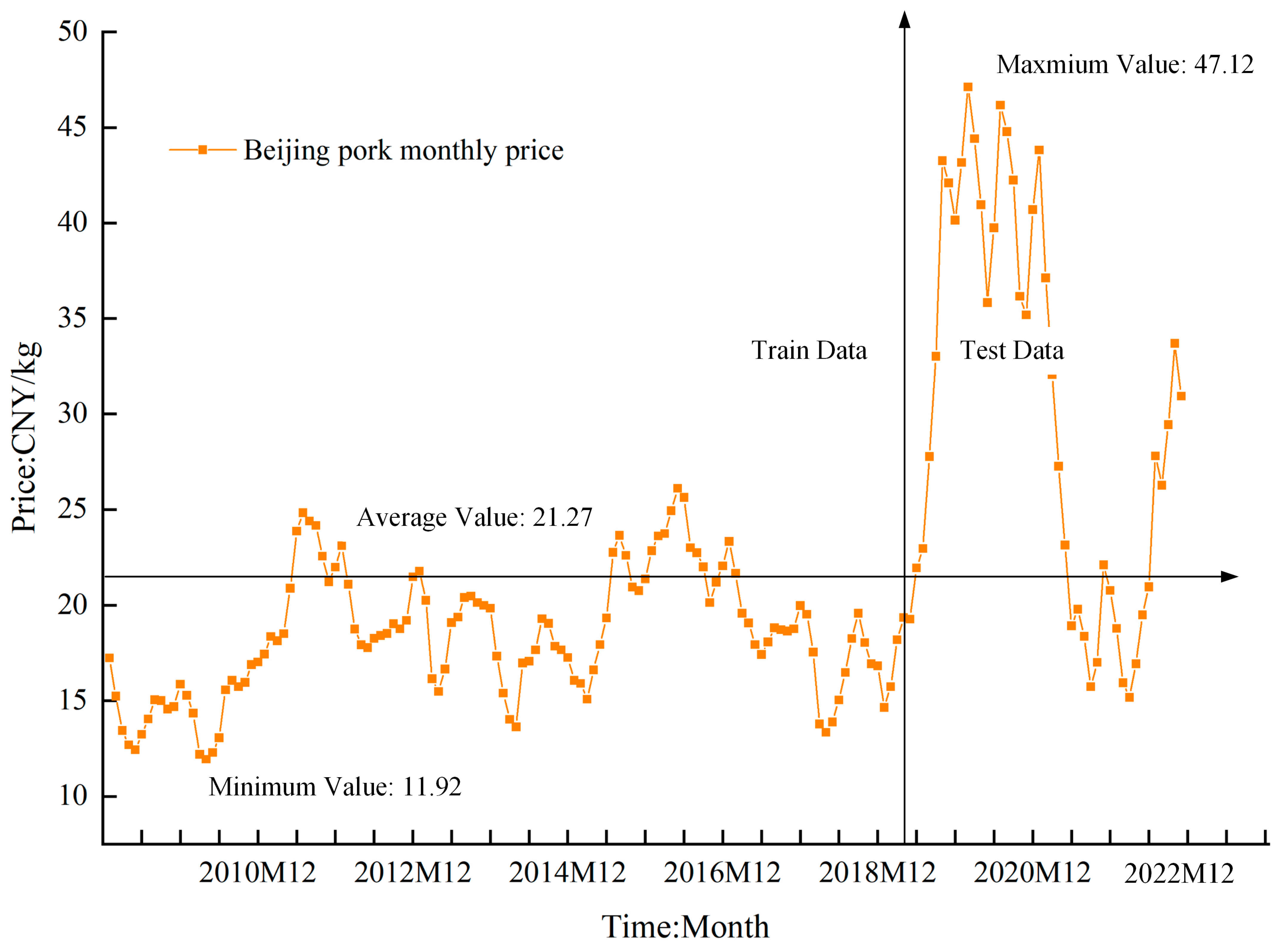
4.1. Data Source

The data used in this study were monthly Beijing pork price data obtained from the Beijing Statistics Information Center, and the sampling interval spanned from January 2009 to September 2024, a total of 189 months. The highest was 47.12 CNY/kg in February 2020, and the lowest was 11.92 CNY/kg in April 2010, with a difference of 35.2 CNY/kg (Figure 3). Seventy percent of the entire dataset (ranging from January 2009 to September 2020) was set as the training set for the model, while the remaining thirty percent (from October 2020 to September 2024) was assigned as the test set to assess the model’s predictive performance.

4.2. Evaluation Metrics

To assess the accuracy of the models’ predictions, various metrics were employed, like the mean absolute error (MAE), mean absolute percentage error (MAPE), mean squared error (MSE), root mean squared error (RMSE), and Theil’s inequality coefficient (TIC). These metrics serve as indicators of predictive error, and lower values signify improved predictive accuracy [2,11,38]. The formulas for each of these indicators are provided below.
M A E = 1 m i = 1 m k i k i
M A P E = 1 m i = 1 m ( k i k i ) / k i × 100 %
M S E = 1 m i = 1 m ( k i k i ) 2
R M S E = 1 m i = 1 m ( k i k i ) 2
T I C = 1 m i = 1 m ( k i k i ) 2 1 m i = 1 m k i 2 + 1 m i = 1 m k i 2
In these equations, k i is the actual value at time i , k i is the predicted value at time i , and m is the number of predicted data points.

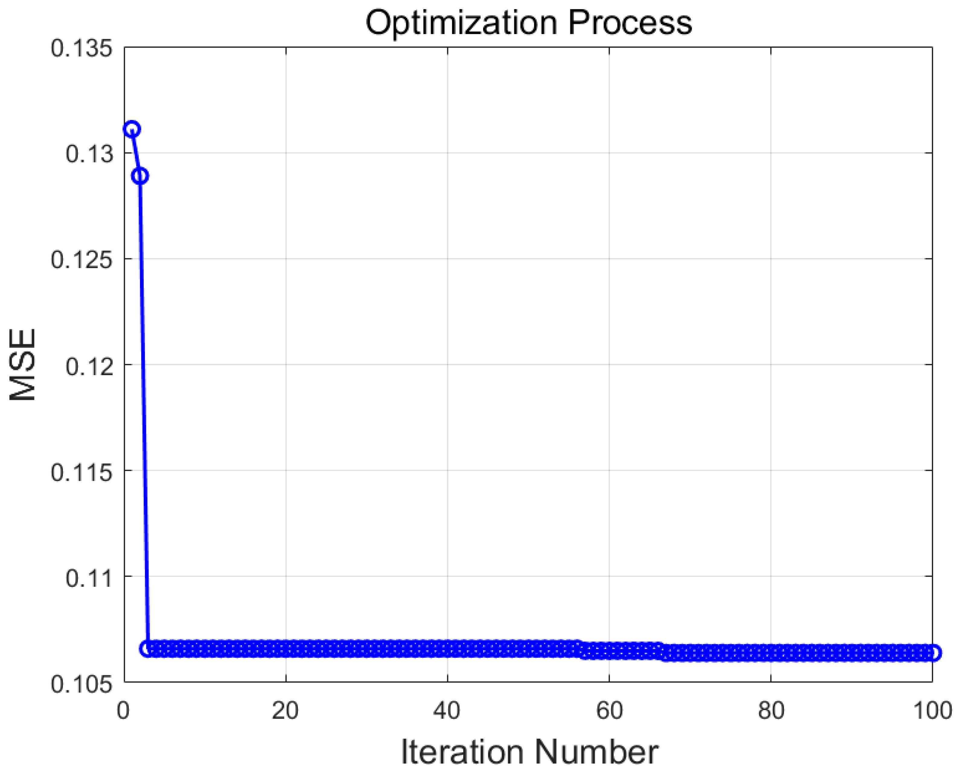
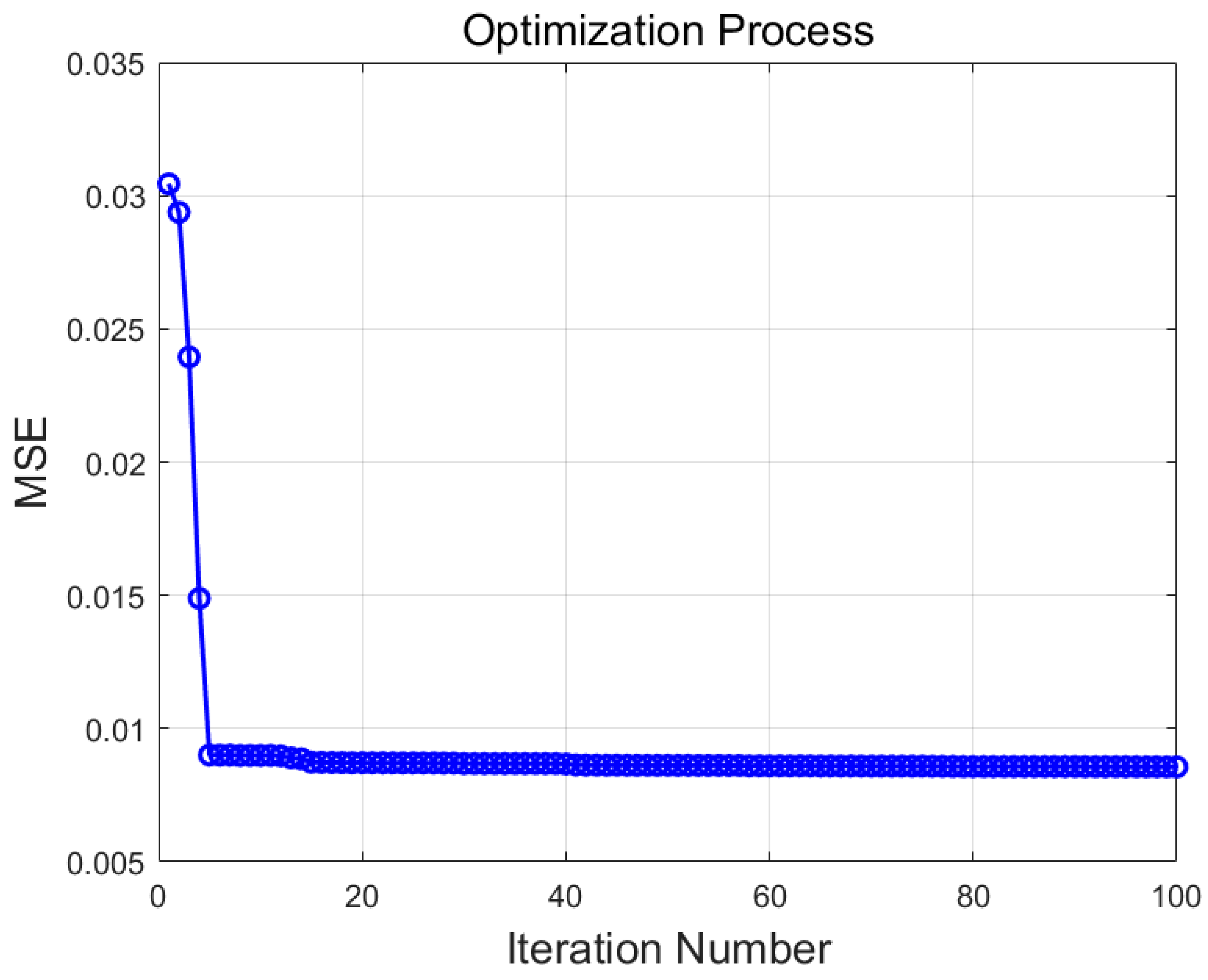
4.3. SSA Optimization Process for the SVR and ELM

The SSA parameters were configured with a population size of 20, and the algorithm was designed to iterate a maximum of 100 times. The proportion of discoverers, labeled as P D N u m , constituted 70% of the total population, while the proportion of sparrows assigned to detection and warning, labeled as S D N u m , was 20% of the total population. The alarm threshold, labeled as S T , was fixed at 0.6. The computational setup consisted of an AMD Ryzen 9 5900 HX processor with AMD Radeon™ Graphics operating at 3.30 GHz, equipped with 32 GB of RAM, running the Windows 11 operating system, and utilizing the MATLAB R2020b environment for simulation experiments. Figure 4 and Figure 5 display the MSE convergence situations.
Figure 4 and Figure 5 demonstrate that the MSE of the SSA-optimized SVR converged in three generations with a value of 0.1066. Furthermore, the MSE of the SSA-optimized ELM converged in 30 generations with a value of 0.0087. The training errors for both the SSA-optimized SVR and ELM models decreased progressively as the number of iterations increased, suggesting that the SSA was effectively escaping local optima in its search for the global optimum during the training phase, thereby enhancing the predictive accuracy of the models.

4.4. Combined Prediction Model Weighting Vector Determination

As shown in Table 1, the mean accuracies for the SVR, ELM, SSA-SVR, and SSA-ELM models were 0.12, 0.44, 0.53, and 0.65, respectively. The SSA-optimized models (SSA-SVR and SSA-ELM) outperformed the original SVR and ELM models in terms of average precision. Specifically, the SSA-ELM model achieved the highest mean residual accuracy in pork price forecasting, while the SVR and ELM models had relatively lower accuracy.
Table 2 provides details of the evaluation metrics for the residual predictions of each model. The SSA-SVR and SSA-ELM models both achieved higher residual prediction accuracy than their non-SSA counterparts. For the SSA-SVR model, the MAE, MAPE, MSE, RMSE, and TIC values were 1.88, 1.53, 9.87, 3.14, and 0.51, respectively. Compared with the SVR model, the RMSE of the SSA-SVR model decreased by 19.29%. For the SSA-ELM model, these values were 0.63, 1.93, 0.60, 0.77, and 0.09, respectively. Compared to the ELM model, the RMSE of the SSA-ELM model was reduced by 56.10%. These results underscore the importance of parameter tuning in forecasting model development and confirm that SSA significantly enhances the predictive accuracy of both SVR and ELM models.
Due to the superior predictive accuracy of the SSA-SVR and SSA-ELM models compared to the traditional SVR and ELM models, these optimized models were chosen to undertake the ensemble prediction of the residuals from the GRNN model. The combined forecast using the IOWA method was determined according to Equation (7). The detailed calculation procedure is as follows.
f L ( a 1 , 1 , x 11 , a 21 , x 21 ) = f L ( 0.99 , 2.45 , 0.64 , 3.31 ) = 2.45 l 1 3.31 l 2
f L ( a 1 , 2 , x 1 , 2 , a 2 , 2 , x 2 , 2 ) = f L ( 0.74 , 2.23 , 0.91 , 2.72 ) = 2.23 l 2 2.72 l 1
f L ( a 1 , 38 , x 1 , 38 , a 2 , 38 , x 2 , 38 ) = f L ( 0.41 , 2.34 , 0.91 , 5.11 ) = 2.34 l 2 + 5.11 l 1
f L ( a 1 , 39 , x 1 , 39 , a 2 , 39 , x 2 , 39 ) = f L ( 0.54 , 2.23 , 0.92 , 4.43 ) = 2.23 l 2 + 4.43 l 1
By substituting these equations into Equation (8), the optimal model under the minimum error sum of squares criterion can be obtained as follows.
min S ( l 1 , l 2 ) = t = 1 39 x t f L ( a 1 , t , x 1 , t , a 2 , t , x 2 , t ) 2 s . t . l 1 + l 2 = 1 l 1 0 , l 2 0
where x t ( t = 1 , 2 , , 39 ) is the residual data of the pork price series, and the optimal weight coefficients l 1 ,   l 2 are obtained by using the planning solution. The optimal weight coefficients of the IOWA-based optimal neural network residual correction prediction model were calculated as l 1 = 0.307 ,   l 2 = 0.693 .

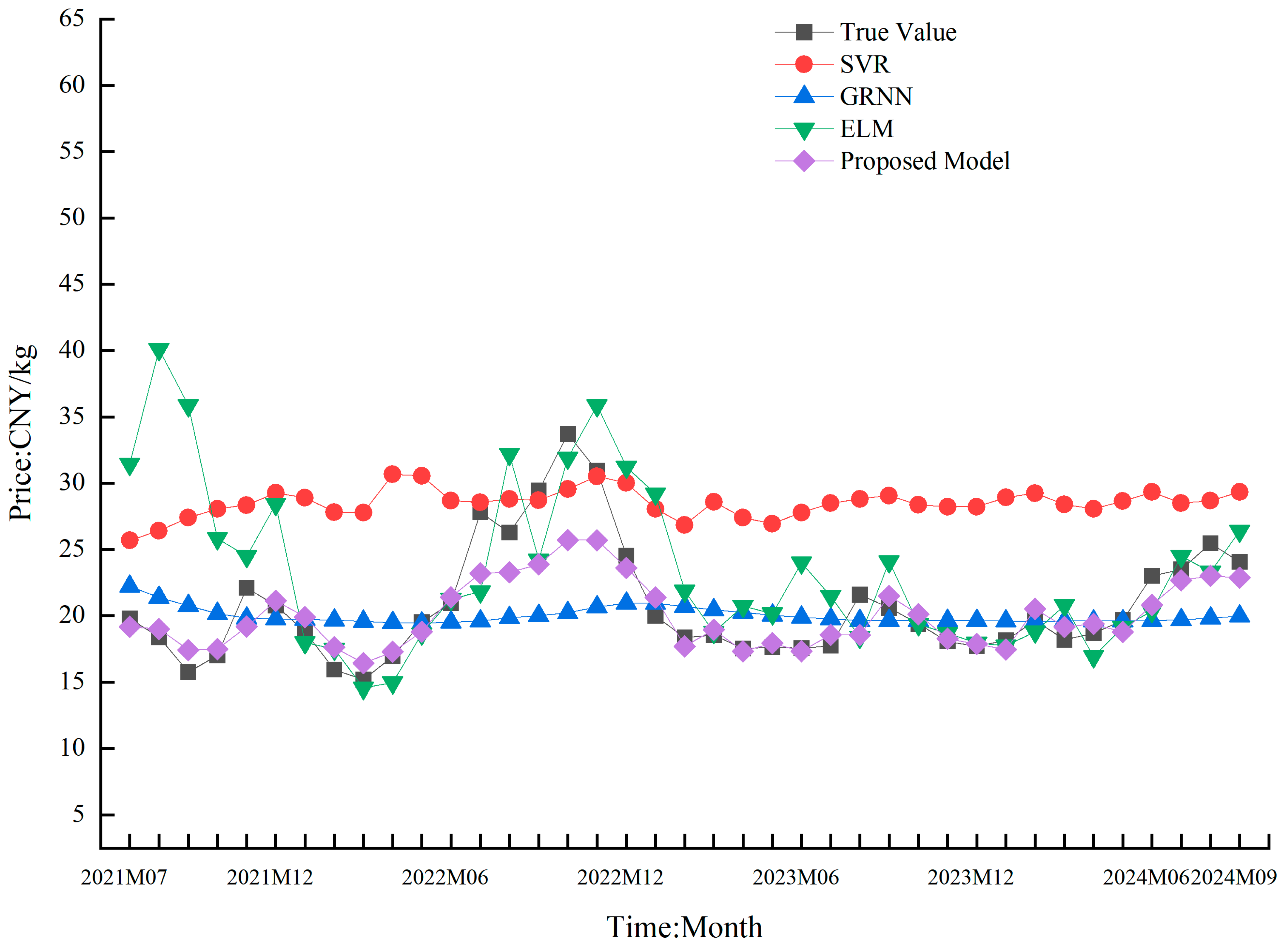
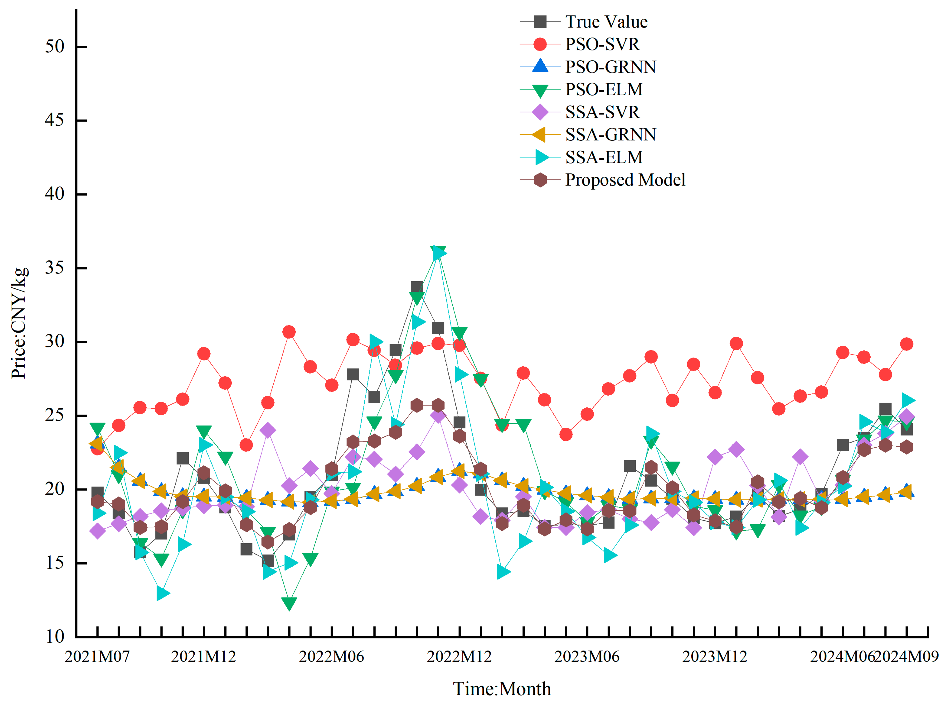
4.5. Comparison of the Results of Different Prediction Models

To evaluate the performance of the models, a comparison of the predictive capabilities of the SVR, GRNN, ELM, PSO-SVR, PSO-GRNN, PSO-ELM, SSA-SVR, SSA-GRNN, and SSA-ELM models was made using monthly pork price data from Beijing. The accuracy of the predictions of these ten models was ascertained in accordance with Equations (12)–(16). The fitting effects of the models are presented in Figure 6 and Figure 7, while Table 3 shows the performance of the models based on evaluation metrics such as MAE, MAPE, MSE, RMSE, and TIC.
(1) Analysis of the results of single prediction models
There were different degrees of fluctuations in the prediction results of the SVR, GRNN, and ELM models. The GRNN model achieved the best prediction results, followed by the ELM and SVR models, respectively. The MAE, MAPE, MSE, RMSE, and TIC values of the GRNN model were 3.17, 0.14, 18.45, 4.30, and 0.10, respectively. Relative to the SVR model, the GRNN model exhibited decreases of 75.54% and 50.54% in the MSE and RMSE metrics, respectively. Relative to the ELM model, the GRNN model exhibited decreases of 53.66% and 31.92% in the MSE and RMSE metrics, respectively. This indicates that the GRNN model achieved good predictive performance relative to the SVR and ELM models.
(2) Analysis of the results of individual prediction models
The PSO-SVR, PSO-GRNN, and PSO-ELM models manifested significantly enhanced predictive performance in contrast to their non-optimized equivalents, namely the SVR, GRNN, and ELM models, respectively. Particularly, the PSO-ELM model had RMSE and TIC values of 3.29 and 0.08 respectively. Compared with the PSO-SVR and PSO-GRNN models, the PSO-ELM model demonstrated a reduction in the RMSE value by 55.55% and 18.94%, respectively.
When contrasted with the SVR model, the PSO-SVR presented reductions in both the MSE and RMSE by 27.41% and 14.80%, respectively. Particle swarm optimization (PSO) has been effectively utilized to finely adjust the parameters of SVR models, generating positive results [39]. Compared with the GRNN model, the PSO-GRNN model accomplished a decrease in MSE and RMSE by 10.76% and 5.54%, respectively. When pitted against the ELM model, the PSO-ELM model saw a more significant drop in MSE and RMSE by 72.83% and 47.88%, respectively. The combination of ensemble empirical modal decomposition (EEMD) and PSO for displacement prediction has been noted to surpass the accuracy of ELM and PSO-BPNN models [22]. The predictive capabilities of the SVR, GRNN, and ELM models were enhanced through PSO optimization of their parameters. The parameter optimization of SVR, GRNN, and ELM was facilitated by PSO’s robust global search capability and swift convergence [31,40].
The SSA-SVR, SSA-GRNN, and SSA-ELM models exhibited significantly enhanced predictive performance in contrast to the standard SVR, GRNN, and ELM models, respectively. Among them, the SSA-ELM model attained the highest degree of predictive accuracy, with MAE, MAPE, MSE, RMSE, and TIC values of 2.18, 0.10, 7.57, 2.75, and 0.07, respectively. When compared to the RMSE values of the SSA-SVR and SSA-GRNN models, the SSA-ELM model displayed a reduction of 24.90% and 30.84%, respectively.
In comparison with the SVR model, the MSE and RMSE values of the SSA-SVR model decreased by 82.21% and 57.82%, respectively. In a previous study, the SSA was used to finely adjust the penalty factors and kernel function parameters of an SVR model for drilling risk assessment, and it was discovered that the model’s accuracy surpassed that of the BPNN [41]. When contrasted to the GRNN model, the MSE and RMSE of the SSA-GRNN model were reduced by 14.27% and 7.41%, respectively. In opposition to the ELM model, the MSE and RMSE of the SSA-ELM model were lessened by 81.00% and 56.41%, respectively. Researchers have previously demonstrated that the SSA-ELM model performed better than the ABC-ELM, PSO-ELM, and GA-ELM models in terms of accuracy in evapotranspiration prediction [42]. These results emphasize the importance of parameter optimization for the SVR, GRNN, and ELM models, mainly because the SSA is outstanding in search accuracy, convergence speed, stability, and the avoidance of local optima, thereby effectively optimizing model parameters and enhancing the models’ predictive capabilities [24,42].
(3) Analysis of the results of combined prediction models
Table 3 shows that there were differences in the fit quality among the 10 predictive models, and the optimal neural network residual correction prediction method using the IOWA operator achieved the best fit. The proposed model presented the MAE, MAPE, MSE, RMSE, and TIC values of 1.52, 0.07, 5.20, 2.28, and 0.06, respectively. Compared with the SVR, GRNN, and ELM models, the RMSE of the proposed model showed reductions of 73.76%, 46.94%, and 63.88%, respectively. When contrasted to the PSO-SVR, PSO-GRNN, PSO-ELM, SSA-SVR, SSA-GRNN, and SSA-ELM models, the RMSE of the proposed model exhibited decreases of 69.20%, 43.83%, 30.70%, 37.77%, 42.69%, and 17.14%, respectively. This indicates that the proposed model has achieved varying levels of enhancement in predictive outcomes. Compared with the PSO-SVR, PSO-GRNN, PSO-ELM, SSA-SVR, SSA-GRNN, and SSA-ELM models, the proposed model was found to have lower MAE, RMSE, MAPE, and TIC values. Therefore, the predictive performance of the proposed model is good, and the model can better capture the complex characteristics of agricultural product prices. Thus, it can obtain more accurate forecasting results.

4.6. Forecast of Agricultural Product Prices in the Coming Period

The prediction model that employs the IOWA operator for optimal neural network residual correction was utilized to forecast pork prices for the forthcoming nine-month period, spanning from October 2024 to December 2025 (as detailed in Table 4). The analysis of the projected pork prices for the latter half of 2024 indicates a general upward trend with fluctuations, reaching a peak in December 2024, followed by an overall downward trend, aligning with the pig production cycle. This alignment suggests that the proposed method of optimal neural network residual correction prediction based on the IOWA operator offers practical and valuable guidance for reference.

5. Conclusions

The data regarding agricultural prices in wholesale markets possess characteristics of nonlinearity and cyclicality, making the accurate prediction of these prices essential for producers to adjust their production plans and guarantee the stability of agricultural market prices. To overcome the limitations of individual forecasting models in capturing all the subtleties of agricultural price series and their frequently insufficient forecasting accuracy, this study introduces a prediction approach that depends on combined residual correction. This research presents two major innovations. Firstly, the input weights and hidden layer biases of the ELM model are assigned randomly, and these assignments can affect the model’s convergence speed and accuracy. In the proposed method, the SSA is utilized to optimize the weights and thresholds of the ELM model, thereby enhancing its generalization ability and predictive accuracy. Secondly, the penalty factors and kernel function parameters have a significant influence on the predictive performance of the SVR model. In the proposed method, the SSA is employed to optimize these parameters for the SVR, with the aim of enhancing its generalization ability and prediction accuracy. Finally, considering that the prediction accuracy of a single model can fluctuate over time, with periods of high and low accuracy, this study introduces the use of the IOWA operator. This operator combines the predicted residuals’ weights from the SSA-SVR and SSA-ELM models to calculate the combined residual prediction value at each point in the sample interval, further improving the forecast results of the GRNN model.
To assess the effectiveness of the models, monthly pork price data from Beijing spanning January 2009 to September 2024 were selected for analysis. A comparative study was conducted on the predictive performance of nine models: SVR, GRNN, ELM, PSO-SVR, PSO-GRNN, PSO-ELM, SSA-SVR, SSA-GRNN, and SSA-ELM. The findings revealed that the PSO-SVR, PSO-GRNN, and PSO-ELM models achieved higher predictive accuracy compared to the standard SVR, GRNN, and ELM models, respectively. In a similar vein, the SSA-SVR, SSA-GRNN, and SSA-ELM models also demonstrated improved predictive accuracy over the standard SVR, GRNN, and ELM models, respectively. This indicated that both PSO and SSA are capable of effectively tuning the parameters of the SVR, GRNN, and ELM models, thereby enhancing their predictive accuracy.
In order to verify the validity of the models, data on the monthly pork price in Beijing from January 2009 to September 2024 were chosen, and the forecasting effects of nine models, namely the SVR, GRNN, ELM, PSO-SVR, PSO-GRNN, PSO-ELM, SSA-SVR, SSA-GRNN, and SSA-ELM models, were compared. The results indicated that the prediction accuracies of the PSO-SVR, PSO-GRNN, and PSO-ELM models were, respectively, higher than those of the SVR, GRNN, and ELM models. Moreover, the prediction accuracies of the SSA-SVR, SSA-GRNN, and SSA-ELM models were higher than those of the SVR, GRNN, and ELM models, respectively. It was demonstrated that PSO and the SSA can effectively optimize the parameters of the SVR, GRNN, and ELM models and improve the model prediction accuracy. Compared with the SVR, GRNN, ELM, PSO-SVR, PSO-GRNN, PSO-ELM, SSA-SVR, SSA-GRNN, and SSA-ELM models, the proposed model exhibited variable degrees of decrease in the MAE, MAPE, MSE, RMSE, and TIC values. This proves that the proposed model is able to capture the characteristics of pork price fluctuation changes and more accurately predict the prices.
The effectiveness of the proposed optimal neural network residual prediction forecasting method based on the IOWA operator in the prediction of pork prices was verified. Agricultural product price prediction is a complex multidimensional nonlinear problem. The impacts on agricultural product prices not only include the influences of supply and demand, costs, and exogenous market factors, but also the influences of unpredictable factors such as import and export trade and national policies. In the future, multi-factor prediction models for agricultural product price prediction can be constructed. Considering the complexity of agricultural commodity prices, they will be decomposed in future research, and a combined agricultural commodity price forecasting model will be constructed.

Author Contributions

B.L.: conceptualization, methodology, software, and writing—original draft preparation. Y.L.: data curation, and data collection and visualization. All authors have read and agreed to the published version of the manuscript.

Funding

This research was funded by the Yangzhou University High-Level Talent Research Initiation Project (137013600).

Data Availability Statement

The original contributions presented in this study are included in the article. Further inquiries can be directed to the corresponding author.

Conflicts of Interest

The authors declare that they have no known competing financial interests or personal relationships that could have appeared to influence the work reported in this paper.

References

  1. Jin, Y.; Li, W.; Gil, J.M. Forecasting fish prices with an artificial neural network model during the tuna fraud. J. Agric. Food Res. 2024, 18, 101340. [Google Scholar] [CrossRef]
  2. Zhang, D.; Zang, G.; Li, J.; Ma, K.; Liu, H. Prediction of soybean price in China using QR-RBF neural network model. Comput. Electron. Agric. 2018, 154, 10–17. [Google Scholar] [CrossRef]
  3. Xiong, T.; Li, C.; Bao, Y. Seasonal forecasting of agricultural commodity price using a hybrid STL and ELM method: Evidence from the vegetable market in China. Neurocomputing 2018, 275, 2831–2844. [Google Scholar] [CrossRef]
  4. Li, B.; Ding, J.; Yin, Z.; Li, K.; Zhao, X.; Zhang, L. Optimized neural network combined model based on the induced ordered weighted averaging operator for vegetable price forecasting. Expert Syst. Appl. 2021, 168, 114232. [Google Scholar] [CrossRef]
  5. Shukur, O.B.; Lee, M.H. Daily wind speed forecasting through hybrid KF-ANN model based on ARIMA. Renew. Energy 2015, 76, 637–647. [Google Scholar] [CrossRef]
  6. Tealab, A. Time series forecasting using artificial neural networks methodologies: A systematic review. Future Comput. Inform. J. 2018, 3, 334–340. [Google Scholar] [CrossRef]
  7. Fallah Tehrani, A.; Ahrens, D. Enhanced predictive models for purchasing in the fashion field by using kernel machine regression equipped with ordinal logistic regression. J. Retail. Consum. Serv. 2016, 32, 131–138. [Google Scholar] [CrossRef]
  8. Zhu, H.; Xu, R.; Deng, H. A novel STL-based hybrid model for forecasting hog price in China. Comput. Electron. Agric. 2022, 198, 107068. [Google Scholar] [CrossRef]
  9. Esen, H.; Ozgen, F.; Esen, M.; Sengur, A. Artificial neural network and wavelet neural network approaches for modelling of a solar air heater. Expert Syst. Appl. 2009, 36, 11240–11248. [Google Scholar] [CrossRef]
  10. Jha, G.K.; Sinha, K. Time-delay neural networks for time series prediction: An application to the monthly wholesale price of oilseeds in India. Neural Comput. Appl. 2012, 24, 563–571. [Google Scholar] [CrossRef]
  11. Liu, Y.; Duan, Q.; Wang, D.; Zhang, Z.; Liu, C. Prediction for hog prices based on similar sub-series search and support vector regression. Comput. Electron. Agric. 2019, 157, 581–588. [Google Scholar] [CrossRef]
  12. Yao, X.; Wang, Z.; Zhang, H. Prediction and identification of discrete-time dynamic nonlinear systems based on adaptive echo state network. Neural Netw. 2019, 113, 11–19. [Google Scholar] [CrossRef] [PubMed]
  13. Zaghloul, M.; Barakat, S.; Rezk, A. Predicting E-commerce customer satisfaction: Traditional machine learning vs. deep learning approaches. J. Retail. Consum. Serv. 2024, 79, 103865. [Google Scholar] [CrossRef]
  14. Bates, J.M.; Granger, C.W.J. The Combination of Forecasts. J. Oper. Res. Soc. 1969, 20, 451–468. [Google Scholar] [CrossRef]
  15. Nowotarski, J.; Liu, B.; Weron, R.; Hong, T. Improving short term load forecast accuracy via combining sister forecasts. Energy 2016, 98, 40–49. [Google Scholar] [CrossRef]
  16. Zhang, J.; Tan, Z.; Wei, Y. An adaptive hybrid model for short term electricity price forecasting. Appl. Energy 2020, 258, 114087. [Google Scholar] [CrossRef]
  17. Song, C.; Fu, X. Research on different weight combination in air quality forecasting models. J. Clean. Prod. 2020, 261, 121169. [Google Scholar] [CrossRef]
  18. Wang, J.; Wang, Z.; Li, X.; Zhou, H. Artificial bee colony-based combination approach to forecasting agricultural commodity prices. Int. J. Forecast. 2019, 38, 1–14. [Google Scholar] [CrossRef]
  19. Zhang, Y.; Song, Y.; Wei, G. A feature-enhanced long short-term memory network combined with residual-driven ν support vector regression for financial market prediction. Eng. Appl. Artif. Intell. 2023, 118, 105663. [Google Scholar] [CrossRef]
  20. Hu, R.; Wen, S.; Zeng, Z.; Huang, T. A short-term power load forecasting model based on the generalized regression neural network with decreasing step fruit fly optimization algorithm. Neurocomputing 2017, 221, 24–31. [Google Scholar] [CrossRef]
  21. Wu, W.; Chen, K.; Tsotsas, E. Prediction of particle mixing in rotary drums by a DEM data-driven PSO-SVR model. Powder Technol. 2024, 434, 119365. [Google Scholar] [CrossRef]
  22. Du, H.; Song, D.; Chen, Z.; Shu, H.; Guo, Z. Prediction model oriented for landslide displacement with step-like curve by applying ensemble empirical mode decomposition and the PSO-ELM method. J. Clean. Prod. 2020, 270, 122248. [Google Scholar] [CrossRef]
  23. Adnan, R.M.; Mostafa, R.; Kisi, O.; Yaseen, Z.M.; Shahid, S.; Zounemat-Kermani, M. Improving streamflow prediction using a new hybrid ELM model combined with hybrid particle swarm optimization and grey wolf optimization. Knowl. Based Syst. 2021, 230, 107379. [Google Scholar] [CrossRef]
  24. Xue, J.; Shen, B. A novel swarm intelligence optimization approach: Sparrow search algorithm. Syst. Sci. Control Eng. Open Access J. 2020, 8, 22–34. [Google Scholar] [CrossRef]
  25. Zhang, C.; Ding, S. A stochastic configuration network based on chaotic sparrow search algorithm. Knowl. Based Syst. 2021, 220, 106924. [Google Scholar] [CrossRef]
  26. Colino, E.V.; Irwin, S.H.; Garcia, P. Improving the accuracy of outlook price forecasts. Agric. Econ. 2011, 42, 357–371. [Google Scholar] [CrossRef]
  27. Mohammadi, H.; Su, L. International evidence on crude oil price dynamics: Applications of ARIMA-GARCH models. Energy Econ. 2010, 32, 1001–1008. [Google Scholar] [CrossRef]
  28. Teste, F.; Makowski, D.; Bazzi, H.; Ciais, P. Early forecasting of corn yield and price variations using satellite vegetation products. Comput. Electron. Agric. 2024, 221, 108962. [Google Scholar] [CrossRef]
  29. Elavarasan, D.; Vincent, D.R.; Sharma, V.; Zomaya, A.Y.; Srinivasan, K. Forecasting yield by integrating agrarian factors and machine learning models: A survey. Comput. Electron. Agric. 2018, 155, 257–282. [Google Scholar] [CrossRef]
  30. Avinash, G.; Ramasubramanian, V.; Ray, M.; Paul, R.K.; Godara, S.; Nayak, G.H.H.; Kumar, R.R.; Manjunatha, B.; Dahiya, S.; Iquebal, M.A. Hidden Markov guided Deep Learning models for forecasting highly volatile agricultural commodity prices. Appl. Soft Comput. 2024, 158, 111557. [Google Scholar] [CrossRef]
  31. Jin, C.; Jin, S.; Qin, L. Attribute selection method based on a hybrid BPNN and PSO algorithms. Appl. Soft Comput. 2012, 12, 2147–2155. [Google Scholar] [CrossRef]
  32. Cui, L.; Tao, Y.; Deng, J.; Liu, X.; Xu, D.; Tang, G. BBO-BPNN and AMPSO-BPNN for multiple-criteria inventory classification. Expert Syst. Appl. 2021, 175, 114842. [Google Scholar] [CrossRef]
  33. Ghritlahre, H.K.; Prasad, R.K. Exergetic performance prediction of solar air heater using MLP, GRNN and RBF models of artificial neural network technique. J. Environ. Manag. 2018, 223, 566–575. [Google Scholar] [CrossRef] [PubMed]
  34. Ni, Y.Q.; Li, M. Wind pressure data reconstruction using neural network techniques: A comparison between BPNN and GRNN. Measurement 2016, 88, 468–476. [Google Scholar] [CrossRef]
  35. Blanc, S.M.; Setzer, T. When to choose the simple average in forecast combination. J. Bus. Res. 2016, 69, 3951–3962. [Google Scholar] [CrossRef]
  36. Wu, R.; Huang, H.; Wei, J.; Ma, C.; Zhu, Y.; Chen, Y.; Fan, Q. An improved sparrow search algorithm based on quantum computations and multi-strategy enhancement. Expert Syst. Appl. 2023, 215, 119421. [Google Scholar] [CrossRef]
  37. Zamfirache, I.A.; Precup, R.E.; Roman, R.C.; Petriu, E.M. Reinforcement Learning-based control using Q-learning and gravitational search algorithm with experimental validation on a nonlinear servo system. Inf. Sci. 2022, 583, 99–120. [Google Scholar] [CrossRef]
  38. Yang, W.D.; Wang, J.Z.; Niu, T.; Du, P. A novel system for multi-step electricity price forecasting for electricity market management. Appl. Soft Comput. 2020, 88, 106029. [Google Scholar] [CrossRef]
  39. Bi, J.; Zhao, M.; Yao, G.; Cao, H.; Feng, Y.; Jiang, H.; Chai, D. PSOSVRPos: WiFi indoor positioning using SVR optimized by PSO. Expert Syst. Appl. 2023, 222, 119778. [Google Scholar] [CrossRef]
  40. Xie, K.; Yi, H.; Hu, G.; Li, L.; Fan, Z. Short-term power load forecasting based on Elman neural network with particle swarm optimization. Neurocomputing 2020, 416, 136–142. [Google Scholar] [CrossRef]
  41. Liang, H.; Zou, J.; Li, Z.; Khan, M.J.; Lu, Y. Dynamic evaluation of drilling leakage risk based on fuzzy theory and PSO-SVR algorithm. Future Gener. Comput. Syst. 2019, 95, 454–466. [Google Scholar] [CrossRef]
  42. Jia, Y.; Su, Y.; Zhang, R.; Zhang, Z.; Lu, Y.; Shi, D.; Xu, C.; Huang, D. Optimization of an extreme learning machine model with the sparrow search algorithm to estimate spring maize evapotranspiration with film mulching in the semiarid regions of China. Comput. Electron. Agric. 2022, 201, 107298. [Google Scholar] [CrossRef]
Figure 1. The flow chart of SVR optimization by the SSA.
Applsci 15 05575 g001
Figure 2. The flow chart of ELM optimization by the SSA.
Applsci 15 05575 g002
Figure 3. The monthly price of pork in Beijing from 2010–2024.
Applsci 15 05575 g003
Figure 4. The convergence of the MSE in the SSA-SVR model.
Applsci 15 05575 g004
Figure 5. The convergence of the MSE in the SSA-ELM model.
Applsci 15 05575 g005
Figure 6. Pork price predictions based on four different methods.
Applsci 15 05575 g006
Figure 7. Pork price predictions based on seven different methods.
Applsci 15 05575 g007
Table 1. The predicted residual values and prediction accuracy of the four models.
MonthResidual Actual Value Pork Price (CNY /kg)Residual Prediction ValuePrediction Accuracy
Pork Price (CNY/kg)
SVRELMSSA-SVRSSA-ELMSVRELMSSA-SVRSSA-ELM
2021M07−2.440.14−2.08−2.45−3.310.000.850.990.64
2021M08−3.010.11−2.53−2.23−2.720.000.840.740.91
2021M09−5.030.00−2.09−2.38−5.540.000.420.470.90
2021M10−3.160.13−2.15−2.57−2.960.000.680.810.94
2021M112.280.280.50−1.822.010.120.220.000.88
2021M121.010.33−0.251.201.440.320.000.810.58
2022M01−0.940.221.190.74−1.110.000.000.000.82
2022M02−3.730.07−1.42−1.36−3.620.000.380.360.97
2022M03−4.390.04−5.39−2.47−4.620.000.770.560.95
2022M04−2.540.14−2.38−2.35−2.140.000.940.920.84
2022M050.040.27−1.63−0.14−0.910.000.000.000.00
2022M061.460.350.301.282.180.240.200.880.51
2022M078.210.722.552.136.970.090.310.260.85
2022M086.430.628.072.286.090.100.740.350.95
2022M099.440.696.261.439.420.070.660.151.00
2022M1013.460.8711.432.0813.090.060.850.150.97
2022M1110.280.8312.493.079.500.080.780.300.92
2022M123.590.474.092.113.910.130.860.590.91
2023M01−0.950.22−2.00−0.771.000.000.000.810.00
2023M02−2.340.15−3.13−2.53−3.230.000.660.920.62
2023M03−1.910.17−1.13−2.11−1.260.000.590.900.66
2023M04−2.730.13−3.64−2.53−3.110.000.670.930.86
2023M05−2.400.14−2.94−2.61−1.860.000.770.910.78
2023M06−2.320.10−3.37−2.50−2.580.000.550.920.89
2023M07−2.000.16−2.16−2.06−0.790.000.920.970.40
2023M081.970.36−0.08−1.720.420.180.000.000.21
2023M090.960.322.310.782.340.340.000.810.00
2023M10−0.270.260.250.73−0.160.000.000.000.60
2023M11−1.590.190.82−1.35−1.450.000.000.850.91
2023M12−1.910.17−0.85−2.05−1.620.000.450.930.85
2024M01−1.440.19−0.88−1.48−2.430.000.610.970.31
2024M020.040.280.79−0.151.410.000.000.000.00
2024M03−1.420.200.530.40−2.360.000.000.000.33
2024M04−0.930.220.29−1.120.190.000.000.800.00
2024M050.06−0.470.71−1.86−0.380.000.000.000.00
2024M063.393.530.560.572.600.960.170.170.77
2024M073.804.283.312.434.180.870.870.640.90
2024M085.643.984.852.345.110.710.860.410.91
2024M094.107.086.042.234.430.280.530.540.92
Mean 0.120.440.530.65
Table 2. The evaluation metrics of four methods regarding the residual prediction.
Prediction ModelMAEMAPEMSERMSETIC
SVR2.821.3815.163.890.66
ELM1.422.313.101.760.21
SSA-SVR1.881.539.873.140.51
SSA-ELM0.631.930.600.770.09
Table 3. The evaluation metrics of different methods.
Prediction Model MAE MAPE MSE RMSE TIC
SVR8.040.4375.438.690.17
GRNN3.170.1418.454.300.10
ELM4.090.2139.826.310.14
PSO-SVR6.850.3654.767.400.15
PSO-GRNN2.930.1316.474.060.10
PSO-ELM2.600.1310.823.290.08
SSA-SVR2.640.1213.423.660.09
SSA-GRNN2.880.1315.823.980.10
SSA-ELM2.180.107.572.750.07
Proposed model1.520.075.202.280.06
Table 4. The pork price forecasts for the next nine periods.
Month Forecasted Value (CNY/kg) Month Forecasted Value (CNY/kg)
2024M1021.372025M0617.95
2024M1121.492025M0717.39
2024M1222.072025M0818.55
2025M0119.812025M0920.04
2025M0218.132025M1017.37
2025M0319.392025M1117.11
2025M0418.202025M1216.84
2025M0517.92
Disclaimer/Publisher’s Note: The statements, opinions and data contained in all publications are solely those of the individual author(s) and contributor(s) and not of MDPI and/or the editor(s). MDPI and/or the editor(s) disclaim responsibility for any injury to people or property resulting from any ideas, methods, instructions or products referred to in the content.

