Machine Learning for the Prediction of Thermodynamic Properties in Amorphous Silicon

Abstract

This study integrated molecular dynamics (MD) simulations with machine learning techniques, specifically Linear, Ridge, and Support Vector Regression, to predict the thermodynamic properties of amorphous silicon (a-Si) under varying conditions. The MD simulations provided a detailed dataset that captured the atomic-level behavior of the a-Si, which enabled exploration of how thermodynamic factors, such as the cooling rate, temperature, and pressure, affect the material’s density, internal energy, and enthalpy. Machine learning models were trained on this dataset and demonstrated exceptional predictive accuracy with $R^2$ values that exceeded 0.95 and minimal root-mean-square errors. The results reveal that the temperature and pressure significantly influenced the thermodynamic properties of the a-Si, while the cooling rate had a minor effect. The models generated isobaric and isothermal curves, which offered deeper insights into the thermodynamic behavior of the a-Si and complemented traditional MD simulations by providing a more efficient means to explore thermodynamic states. This work highlights the potential of machine learning to accelerate the study of materials by enabling faster exploration of thermodynamic behavior and the generation of additional data. This approach enhances the understanding of the equation of state of a-Si and opens new avenues for applying this hybrid modeling technique to other materials.

1. Introduction

Amorphous silicon (a-Si) is a non-crystalline form of silicon that plays a critical role in various technological applications, including thin-film solar cells, flat-panel displays, and photodetectors [1,2,3]. Its disordered atomic structure endows it with unique electronic and optical properties, making it particularly suitable for devices requiring tunable bandgaps and high absorption coefficients [4,5]. Furthermore, understanding the properties of a-Si is essential for optimizing its performance and stability under different processing and operational conditions. However, accurately predicting these properties remains challenging due to the complex atomic dynamics inherent to amorphous materials.

Molecular dynamics (MD) simulations serve as a valuable tool for exploring a-Si without incurring costly experiments. Various studies have focused on this approach, including thermal conductivity [6], Li-ion diffusion [7], oxidation rates [8], structure and stress during lithiation [9], deformation mechanisms in nanoporous a-Si [10], structural dynamics [11], and the exploration of tension–compression [12], among many others [12,13,14]. While MD simulations provide accurate, atomistic-level insights, they are time-consuming, especially for large systems or long simulation timescales. In this context, machine learning (ML) has emerged as a promising tool for predicting material properties. ML algorithms can efficiently identify complex patterns and relationships within vast datasets, enabling the rapid prediction of material behavior under diverse conditions. Although ML models require training on a previously constructed dataset, once trained, they can make rapid predictions across a wide range of conditions without the need for extensive computational resources. This capability significantly reduces the computational cost and time associated with traditional MD simulations, allowing researchers to explore larger parameter spaces and accelerate materials design. Researchers have developed supervised learning models for predicting the yield stress of high-entropy alloys [15], the Young’s moduli and ultimate tensile strengths of nanocomposites [16], the mechanical properties of metallic glasses [17], and nanoparticle magnetization [18], among others. Physics-informed machine learning has also emerged as a promising approach to overcome the limitations of traditional numerical methods, such as finite element methods, by integrating physical laws with neural networks, enabling the efficient modeling of complex, high-dimensional, and noisy scientific problems [19,20]. In the case of a-Si, the literature is more limited. While there are some studies that have used ML-based interatomic potentials to model a-Si and for phase recognition [21,22,23], no studies have been conducted to date on predicting the properties of a-Si. The integration of ML models with MD simulations offers a powerful hybrid approach, leveraging the accuracy of atomistic simulations with the speed and scalability of data-driven methods, opening new avenues for materials discovery and optimization.

To bridge this gap, 150 MD simulations were performed to calculate the thermodynamic properties of a-Si under different conditions. The resulting data were used to construct a dataset for property prediction using classical regression models. Specifically, the cooling rate, temperature, and pressure served as predictors, while the density, internal energy, and enthalpy were the target variables in the regression models. The models’ effectiveness was demonstrated by analyzing the relationships between these variables across various thermodynamic conditions. This approach not only provided a comprehensive understanding of the impact of these parameters on the thermodynamic behavior of a-Si, but also enabled the identification of trends and anomalies that would be challenging to capture through MD simulations alone. The synergy between MD simulations and ML models allows for the rapid exploration of material properties, paving the way for the more efficient design and optimization of amorphous-silicon-based materials.

2. Materials and Methods

To predict the thermodynamic properties of a-Si, the pipeline was divided into three stages. The first stage involved conducting MD simulations to collect data on various properties of the a-Si. In the second stage, these properties were compiled into a single dataset for data processing. Finally, in the third stage, regression models were constructed using supervised learning. A schematic representation of this pipeline is shown in Figure 1. Each stage is described in detail below.

2.1. MD Simulations

The MD simulations were performed using the Large-scale Atomic/Molecular Massively Parallel Simulator (LAMMPS (version 29 August 2024) [24]). The atomic interactions in the silicon were modeled with the Tersoff potential using the Si parameterization [25], which has been employed to study a-Si and related materials and effectively capture the covalent bonding characteristics of silicon; it has been extensively validated in previous studies on both crystalline and amorphous silicon [26,27,28,29]. A time step of 1 fs was used throughout all the simulations to achieve a balance between numerical stability and computational efficiency to allow for the precise tracking of atomic motion while maintaining reasonable simulation times.

A simulation box with dimensions of $8.7\times 8.7\times 8.7$ nm³ was constructed, which initially contained crystalline Si with a diamond-like structure. While these dimensions might not be large enough to study the mechanical deformation of a-Si or polycrystalline structures [12], they are suitable for studying thermodynamic properties [6], which was the focus of the current work. The chosen system size balanced computational efficiency with accuracy to ensure that the thermodynamic trends observed were representative of the bulk behavior while maintaining feasible simulation times. To prepare the amorphous state, the system was first minimized using the conjugate gradient algorithm to eliminate any unphysical atomic overlaps and reduce residual stresses in the initial crystalline structure. The temperature was ramped up to 3500 K at a rate of ${10}^{13}$ K/s, followed by equilibration at 3500 K for 0.5 ns. Quenching was then performed at a cooling rate of $R_c$ until reaching a temperature of 100 K. These steps were conducted under the NVT ensemble with periodic boundary conditions to eliminate surface effects and simulate bulk-like conditions.

After quenching, the system was further equilibrated at a target temperature T and pressure P for 0.2 ns under the NPT ensemble. This relaxation step ensured that any residual stresses from rapid cooling were dissipated and that the system reached a stable thermodynamic state before the property calculations. To systematically explore the influence of the cooling rate, temperature, and pressure on the thermodynamic properties of the a-Si, a broad set of input conditions was considered. The input variables comprised five values for $R_c$ ($1\times {10}^{11}$, $5\times {10}^{11}$, $1\times {10}^{12}$, $5\times {10}^{12}$, $1\times {10}^{13}$ K/s), five values for T (100, 200, 300, 400, and 500 K), and six values for P (0, 2, 4, 6, 8, and 10 GPa), which resulted in a total of 150 different simulation combinations that encompassed conditions that ranged from standard synthesis environments to high-pressure regimes where structural compaction is expected. These cooling rates were adopted based on previous studies that have shown that they effectively induce amorphization in covalent materials [30,31], while the selected hydrostatic pressures are not high enough to cause plastic deformation of the sample [32].

For each final configuration, key thermodynamic quantities were extracted, namely, the density ($\rho$), internal energy (U), and enthalpy (H), which were selected as the output variables. The dataset generated from these 150 simulations provided a robust foundation for statistical analysis and the development of predictive models using traditional machine learning techniques, such as regression and decision trees [17]. While these methods are effective at identifying trends and interpolating within the sampled parameter space, more complex approaches, such as artificial neural networks, require significantly larger datasets for optimal training. Thus, future studies could expand the dataset to explore deep learning-based modeling strategies for even more accurate predictions of thermodynamic properties.

2.2. Dataset Preparation

All the input and output variables were compiled into a structured dataset that contained 150 observations, where each corresponded to a final configuration obtained from the MD simulations under specific values of $R_c$, T, and P. This dataset is provided in the Supplementary Materials to facilitate reproducibility and further analysis. Given the diverse nature of the variables spanning different orders of magnitude and units (e.g., pressure in GPa, temperature in K, energy in eV, and density in g/cm³), it was necessary to preprocess the data to ensure numerical stability and enhance the performance of the predictive models. To achieve this, standardization was applied to all the variables, transforming them to have a mean of zero and a standard deviation of one. This step mitigated potential biases arising from variables with significantly different scales, allowing the machine learning algorithms to assign equal importance to all the features. The standardization process was carried out using the following expression:

$$z_i^s={\displaystyle \frac{z_i-\mu }{\sigma }},$$

(1)

where $z_i^s$ is the standardized variable; $z_i$ is the original variable from the MD simulations; and $\mu$ and $\sigma$ are the mean and standard deviation of $z_i$, respectively. This transformation ensured that the dataset was centered and scaled appropriately, which improved the convergence and interpretability of the subsequent statistical and ML models. The data handling and transformations were implemented using the Pandas library in Python [33], which provides efficient tools for managing and preprocessing large datasets. While alternative data preprocessing techniques exist, such as min–max normalization, robust scaling, and log transformations, standardization was chosen based on its superior performance in preliminary predictive modeling trials.

2.3. Predictive Models

To develop the predictive models for estimating the thermodynamic properties of the a-Si, we employed Linear, Ridge, and Support Vector Regression (SVR) models [34,35]. These models aimed to establish the mathematical relationships between the input variables ($R_c$, T, and P) and the output properties ($\rho$, U, and H) by facilitating the interpolation and potential extrapolation beyond the simulated data points. Linear regression operates by minimizing the sum of squared residuals to find the best-fit hyperplane that describes the relationships between the predictors and the response variables. While it is one of the most interpretable and widely used regression techniques, it can suffer from instability in the presence of multicollinearity, where predictor variables exhibit strong correlations. This issue may lead to large coefficient magnitudes, making the model sensitive to small variations in the input data and reducing its generalizability. To mitigate this issue, Ridge regression was also employed. Ridge regression introduces an L2 regularization term in the cost function, penalizing large coefficient values and shrinking them toward zero. This approach not only reduces overfitting but also improves the model robustness and lowers the variance, particularly when dealing with high-dimensional or correlated data. The Ridge regression model balances bias and variance by tuning the regularization parameter, ensuring better generalization to unseen data while preserving the predictive power of the model. SVR is based on the principles of Support Vector Machines. However, SVR estimates continuous outputs by minimizing a regularized loss function using an $ϵ$-insensitive margin and support vectors. The three regression tasks were implemented using the Scikit-learn (version 1.4.2) library in Python (version 3.12.4) [36], which provides efficient tools for training, validating, and optimizing predictive models. The predictors $R_c$, T, and P were used to estimate the responses $\rho$, U, and H through the following expressions:

$$\begin{array}{cc}\hfill \rho & ={\omega }_{1,1}{R}_c+{\omega }_{1,2}T+{\omega }_{1,3}P+{\beta }_1,\hfill \end{array}$$

(2)

$$\begin{array}{cc}\hfill U& ={\omega }_{2,1}{R}_c+{\omega }_{2,2}T+{\omega }_{2,3}P+{\beta }_2,\hfill \end{array}$$

(3)

$$\begin{array}{cc}\hfill H& ={\omega }_{3,1}{R}_c+{\omega }_{3,2}T+{\omega }_{3,3}P+{\beta }_3,\hfill \end{array}$$

(4)

where ${\omega }_{i,j}$ and ${\beta }_i$ are the regression coefficients. A 5-fold cross-validation approach was employed to train and test the models. The hyperparameters used in this study can be found in the Supplementary Materials. The performance was assessed using the coefficient of determination $R^2$ and the root-mean-square error (RMSE). $R^2$ was computed using

$$R^2=1-{\displaystyle \frac{{\sum }_{i=1}^n{(y_a-y_p)}^2}{{\sum }_{i=1}^n{(y_a-\overline{y})}^2}},$$

(5)

where n is the total number of observations (150 in this work), $y_a$ is the actual value, $y_p$ is the predicted value, and $\overline{y}$ is the mean of $y_a$. The $R^2$ score ranges from zero (no predictive capability) to one (perfect prediction). The RMSE was calculated using

$$\mathrm{RMSE}=\sqrt{{\displaystyle \frac{1}{n}}{\displaystyle \sum _{i=1}^n}{(y_a-y_p)}^2},$$

(6)

where higher RMSE values indicate a greater deviation between the actual and predicted values, while lower RMSE values reflect more accurate predictions. Although the RMSE is widely used due to its intuitive interpretation in the same units as the target variable, other performance metrics can also offer valuable insights. These include the mean absolute error (MAE), which measures the average absolute difference between the observed and predicted values; mean square error (MSE), which penalizes larger errors more heavily; and mean absolute percentage error (MAPE), which expresses errors as a percentage of actual values, making it useful for relative comparisons. Despite their advantages, these metrics do not share a standardized range like the coefficient of determination ($R^2$), which varies between 0 and 1, facilitating direct comparisons across different models. Instead, the RMSE, MAE, and MSE are scale-dependent, meaning their interpretation depends on the magnitude of the predicted variable. Due to this limitation and to maintain consistency in the model evaluation, only the RMSE and $R^2$ were analyzed in this study, as they provide a balance between interpretability and effectiveness in assessing model performance. In each 5-fold cross-validation iteration, both the $R^2$ and RMSE were calculated for the testing set to evaluate the model performance, and the results were averaged.

3. Results

The data analysis was conducted in two stages to ensure a comprehensive understanding of the system’s behavior. In the first stage, an exploratory analysis was performed on the output variables $\rho$ (density), U (internal energy), and H (enthalpy) to verify their consistency with previously reported results for a-Si. This step also involved examining the relationships between the input variables, cooling rate ($R_c$), temperature (T), and pressure (P), and the output variables to assess how different thermodynamic states emerged from the MD simulations. The second stage focused on developing regression models to predict the $\rho$, U, and H based on the selected input parameters. The predictive capabilities of these models were then evaluated to determine their potential for reconstructing the equations of state, which provided a data-driven approach to understanding the thermodynamic properties of a-Si.

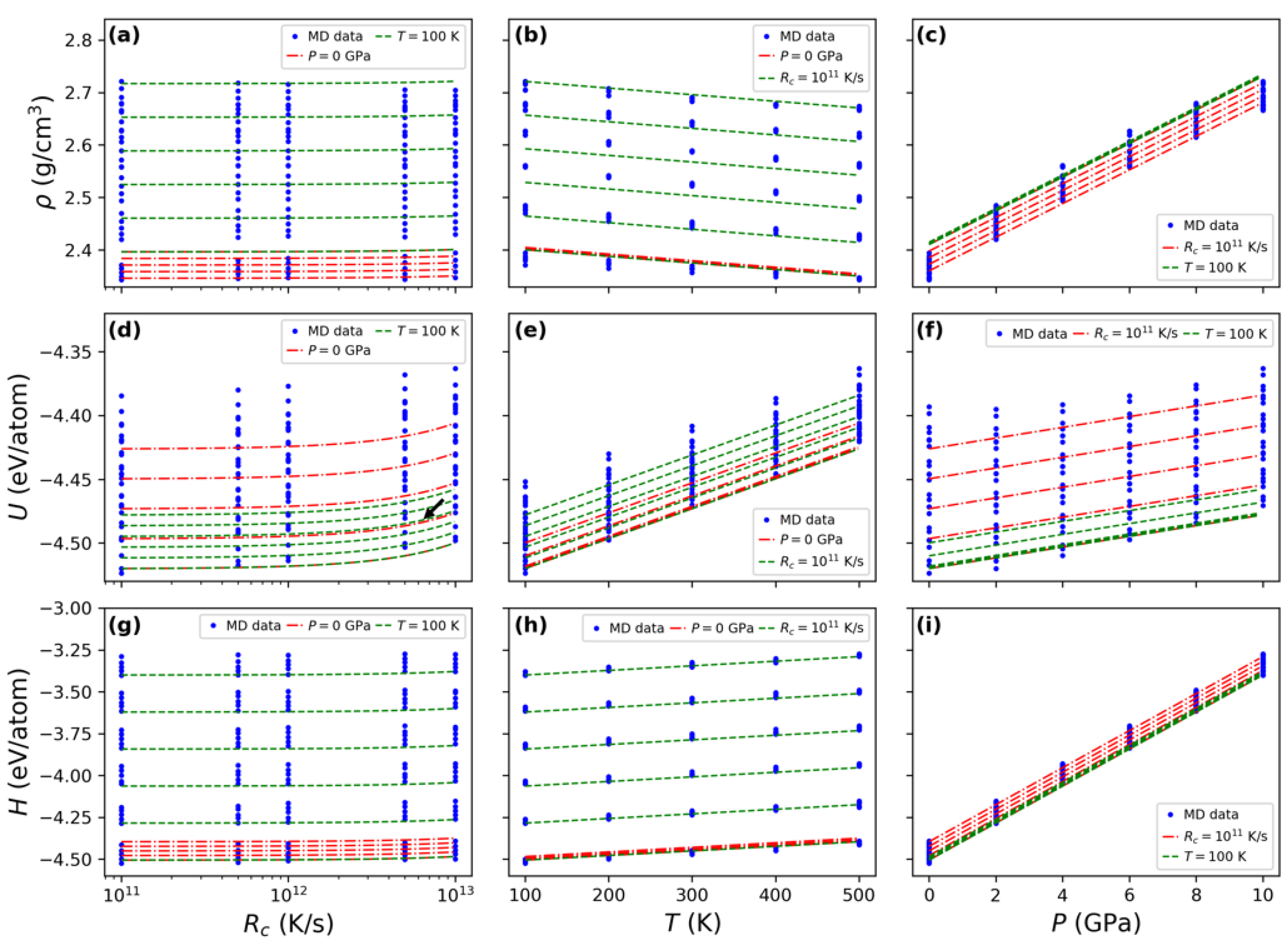
3.1. Statistical Exploration

The values obtained for the $\rho$, U, and H are summarized in the boxplots shown in Figure 2. The density ranged from 2.3 to 2.7 g/cm³, with a median value close to 2.4 g/cm³, which aligned well with previous findings on amorphous silicon [37,38]. The observed lower and upper limits were primarily dictated by the temperature and pressure variations, as is further analyzed in subsequent sections. The internal energy spanned from −4.525 to −4.375 eV/atom, with a median near −4.44 eV/atom. Since U is composed of both potential and kinetic energy components, it is indirectly influenced by pressure and temperature. Structural modifications induced by pressure affect the potential energy landscape, while temperature variations modulate atomic vibrations, increasing the kinetic energy [39,40,41]. Enthalpy exhibits a systematic shift toward higher values relative to internal energy due to the additional contribution of the pressure–volume term in its calculation, as defined by $H=U+PV$. This term accounts for the work associated with maintaining a constant-pressure environment.

The boxplots provided an effective means of statistically exploring the distribution of the thermodynamic variables. By visually representing the central tendency, spread, and presence of potential outliers, these boxplots allowed for an intuitive assessment of variability and underlying trends in the data. They also facilitated direct comparisons between different variables, which helped to identify how external factors, such as the temperature and pressure, influenced the system. Furthermore, the boxplots revealed a relatively uniform distribution of values across all the output variables, which can be attributed to the discrete nature of the input variables—$R_c$, T, and P—rather than stochastic sampling, as outlined in the methodology.

While the boxplots provide an overview of the calculated values, they do not explicitly reveal the influence of the input variables $R_c$, T, and P. To further explore these dependencies, scatter plots illustrating the relationships between the input and output variables were generated, as shown in Figure 3. Due to the discretized selection of input values, the data points appeared evenly distributed rather than randomly scattered. The density $\rho$ exhibited a slightly decreasing trend with $R_c$ and a more pronounced decline with increasing temperature T. This behavior is consistent with previous studies indicating that higher cooling rates lead to an increased free volume, while elevated temperatures enhance atomic vibrations, effectively increasing the atomic spacing [42,43]. Both effects contribute to a reduction in the structural compactness, resulting in lower densities. In contrast, $\rho$ shows a clear increasing trend with pressure P, as compression induces a more compact atomic arrangement [39].

For both the internal energy U and enthalpy H, increasing trends were observed across all the input variables. Higher cooling rates led to higher energy states, which are often associated with structural rejuvenation in amorphous materials [44]. The effects of T and P on the U and H were more direct: increasing temperature raised the kinetic energy component of U, while pressure explicitly influenced the H through the pressure–volume term in its definition. As a reminder, the internal energy is given by $U=Pe+K$, where $Pe$ represents the potential energy and K the kinetic energy. Meanwhile, enthalpy is defined as $H=U+P·V$, highlighting the contribution of work under constant pressure conditions.

The observed relationships between the output variables $\rho$, U, and H and the input parameters T, P, and $R_c$ provides insights into the equations of state, which describe how thermodynamic properties evolve under different conditions. Each data point in the scatter plots represents a specific thermodynamic state of the a-Si, offering a detailed visualization of how structural and energetic properties respond to changes in the cooling rate, temperature, and pressure. These plots serve as a crucial tool for identifying trends, verifying consistency with known physical principles, and providing insights into the interplay between atomic-scale interactions and macroscopic material behavior. Moreover, understanding these dependencies is essential for tailoring processing conditions to achieve desired material properties, particularly in applications where the density, internal energy, or enthalpy play a critical role. However, while the scatter plots effectively capture qualitative trends, obtaining a precise mathematical representation of these relationships requires predictive modeling. The next section presents mathematical models to quantitatively describe these thermodynamic equations of state, enabling more accurate predictions of a-Si behavior under varying conditions.

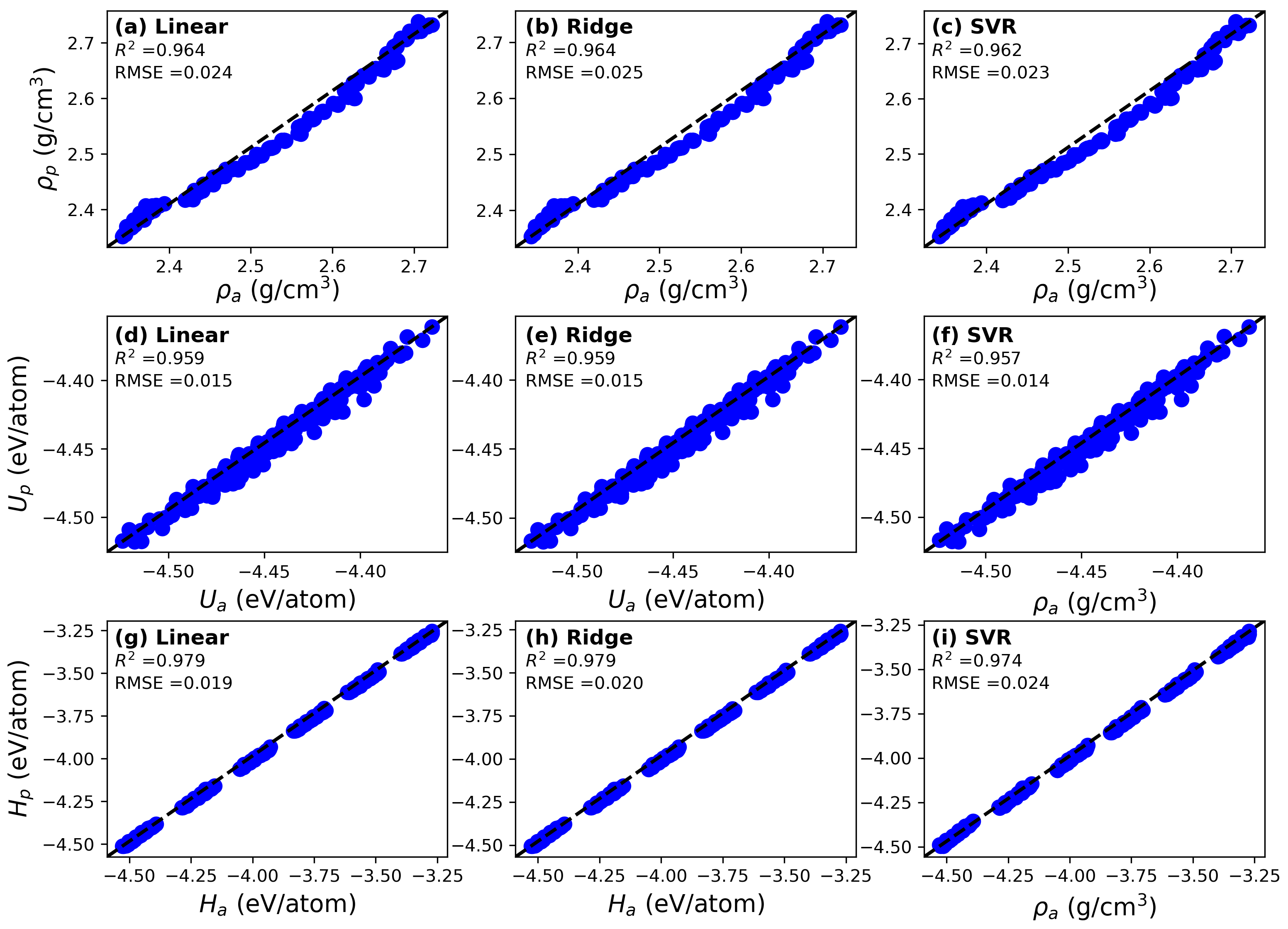
3.2. Predictive Models

As discussed in the previous section, predictive models are essential for obtaining information about the system’s state under different conditions. To achieve this, models were constructed using the $R_c$, T, and P as predictors and the $\rho$, U, and H as responses. The models were trained and tested using five-fold cross-validation, where the dataset was divided into five equal groups. Four groups were used as the training set, and the remaining group served as the testing set. This procedure was repeated, with each group used as the testing set in turn. The model performance was evaluated by calculating the coefficient of determination ($R^2$) and root-mean-square error (RMSE) across all the test sets as follows: First, the three input variables ($R_c$, T, and P) calculated for a given a-Si sample were used by the regression model to predict the values of the density, internal energy, and enthalpy. Then, these predicted values were compared with the actual values obtained from the dataset to compute $R^2$ and RMSE. The predicted and actual values are shown in Figure 4a–c for the $\rho$, Figure 4d–f for the U, and Figure 4g–i for the H, with the standardized variables reverted to their original units for better physical interpretability. In all the cases, the models exhibited excellent performance, where the $R^2$ values exceeded 0.95 and the RMSE values were close to zero, indicating a high predictive accuracy. No significant differences were observed between the three models, suggesting that all approaches were highly effective at predicting the thermodynamic states of the a-Si. A notable observation was that the values in the plots appeared grouped due to the discretized ranges used for the input variables. This grouping was particularly evident for the H, as the pressure (P) was explicitly involved in the calculation of the enthalpy. Exploration of the residuals of the Linear, Ridge, and SVR models can be found in the Supplementary Materials.

While the focus of this study was on the Linear, Ridge, and SVR models, other models were also explored and evaluated using the same cross-validation procedure. Specifically, Lasso regression and Elastic Net were considered. These models extend Ridge regression by incorporating penalty terms into the cost function, which can assist with feature selection and handling highly correlated predictors. However, both the Lasso and Elastic Net models showed lower performances and were excluded from further analysis (see the Supplementary Materials).

To demonstrate the scope of the predictive models developed in this study, we performed predictions for $\rho$, U, and H based on the variables cooling rate, temperature, and pressure using the Linear regression model, which was chosen for its simplicity and interpretability. The following equation was employed:

$$\rho =\left(0.015\right)·R_c-\left(0.159\right)·T+\left(0.984\right)·P+0,$$

(7)

where all the predictors were standardized to a mean of zero and a variance of one. This model was used to generate predictions that were incorporated into the plots shown in Figure 3 by reversing the input and output values to their original units of measure, providing a visual representation of the relationships between the $\rho$ and the input variables. The dotted lines in Figure 5 represent the model’s predictions, which allowed for a clear comparison between the predicted values and the original data from the MD simulations. In particular, the $\rho$–$R_c$ relationship was examined by fixing P at 0 GPa (yielding the $P=0$ GPa curves) and by fixing T at 100 K (resulting in the $T=100$ K curves). This approach allowed for the construction of isobars and isotherms, respectively, which revealed deeper thermodynamic insights into the system’s behavior. For example, varying the cooling rate in the $\rho$ versus T and $\rho$ versus P plots (represented by the red and green curves, respectively) resulted in closely spaced isobars and isotherms. This indicates that the $R_c$ had a relatively minor influence on the thermodynamic states compared with the temperature and pressure, which had more pronounced effects. This is also distinguished in the (a), (d), and (g) panels, where the $R_c$ is the independent variable. As observed, only the U varied significantly when the $R_c$ increased, which is in agreement with previous works that have demonstrated that the cooling rate is explicitly related to the energy states of the sample [44,45]. Additionally, while the H exhibited similar behavior to that of the $\rho$, the U showed an interesting feature: in the U vs. $R_c$ plot shown in panel (d), the isotherms overlap with the isobars. This suggests that increasing the pressure at a constant temperature significantly raised the internal energy, where it eventually equaled that of a state with slightly lower pressure but higher temperature. For instance, the curves for 100 K at 6 GPa and 200 K at 0 GPa (denoted by the black arrow) show comparable internal energy values. The same behavior is observed in the U vs. T plot. While both the U and H share the same units, the H did not display this behavior, which can be attributed to the pressure term in the definition of enthalpy, which resulted in more widely separated values for the H.

While the models accurately replicated the trends observed in the MD data for most variables, they did struggle to fully capture the slight decreasing trend in the $\rho$–$R_c$ relationship. This discrepancy may be attributed to the fact that the relationship between the cooling rate and the density was more subtle and less consistent compared with the stronger trends observed for the temperature and pressure. In contrast, the models were particularly successful in capturing the decreasing trend in the $\rho$–T relationship and the increasing trend in the $\rho$–P relationship, as these patterns were more clearly defined in the data. These observations highlight the capabilities of the models to predict the thermodynamic states with a high degree of accuracy. However, it is important to note that the models were trained within a limited range of variables, and their ability to make accurate predictions outside of this range has not been validated. While the models performed well for the data within the specified ranges, further validation would be necessary to ensure that the predictions remain reliable and robust when applied to conditions outside the training set.

Despite this limitation, the use of ML models presents a significant advantage by allowing for the generation of additional data points that can aid in the reproduction of the equation of state for a material system. Acquiring information for a single state through traditional MD simulations can be computationally expensive and time-consuming, especially when exploring a wide range of conditions. Therefore, ML provides a powerful and efficient tool for predicting thermodynamic properties over a broader spectrum of conditions, enabling faster exploration of the material’s behavior. Additionally, by extending the approach to include data from both the liquid and amorphous phases, it may be possible to investigate the glass-forming ability of the material. This could further expand the utility of the predictive models for studying a wide range of material classes that is not only limited to a-Si but also to other complex systems with varying thermodynamic behaviors.

4. Discussions

The predictive models constructed in this study, which were based on the dataset generated by the MD simulations, demonstrated exceptional performances, as evidenced by $R^2$ values that exceeded 0.95 and minimal root-mean-square errors. These results validate the accuracy and reliability of the models, confirming that they captured the complex relationships between the input variables ($R_c$, T, P) and the thermodynamic outputs, namely, density ($\rho$), internal energy (U), and enthalpy (H). More specifically, the models revealed that while the cooling rate ($R_c$) played a relatively minor role in determining these properties, it still influenced the energy state of the amorphous phase. In contrast, the temperature (T) and pressure (P) had significantly more pronounced impacts: the temperature affected the atomic mobility and energy distribution, while the pressure altered the atomic packing and density, which ultimately determined the material’s behavior. This finding underscores the critical influences of thermal and pressure conditions on the thermodynamic state of a-Si, which is essential for understanding its behavior in various applications, including materials processing and device fabrication.

In addition to validating the accuracy of the models, this study demonstrated the power of machine learning in generating additional thermodynamic data. The models enabled the construction of isobaric and isothermal curves, which provided valuable insights into the material’s behavior under different thermodynamic conditions. These generated curves allowed for a deeper exploration of the thermodynamic properties of the a-Si, particularly by providing a means of examining the relationships between the material’s density, internal energy, and enthalpy at different fixed values of temperature or pressure. This ability to generate data points efficiently and systematically complemented traditional MD simulations, which can be computationally expensive and time-consuming, especially when exploring a broad range of thermodynamic states. By offering a more efficient pathway to explore these properties, the models contributed to a better understanding of the equation of state of the a-Si.

Despite the impressive performance of the models within the training range, it is important to acknowledge their inherent limitations. The considered models were linear, and they were trained within a specific range of variables, and thus, their predictive accuracy outside this range has not been validated. Therefore, careful evaluation and validation of the models are necessary when applying them to thermodynamic conditions beyond the training data. This step is crucial to ensure the robustness and generalizability of the models. For instance, the models could be tested under more extreme or unconventional thermodynamic conditions, such as higher or lower temperatures and pressures, to assess their ability to make reliable predictions in these scenarios. Additionally, including data from additional phases, such as the liquid state, could improve the models and provide a more comprehensive description of phase transitions in a-Si. Predicting phase transitions, such as the transformation from amorphous to crystalline states or the glass-forming ability of the material, could be achieved by incorporating data from both the liquid and amorphous phases. This would allow for the models to be extended to predicting the glass-forming ability of a-Si under various cooling and pressure conditions.

There are several exciting avenues for future work. One promising direction is expanding the dataset to improve the reliability and robustness of the results. Additionally, this dataset could be enriched with further structural descriptors, such as local order parameters, coordination numbers, or bond angles, which would offer a more comprehensive representation of the material’s structural characteristics. By capturing more nuanced relationships between the structure and the thermodynamic properties, these descriptors could enhance the models’ predictive power. Furthermore, incorporating data-driven metrics and fitting theoretical models to observed trends could provide a more quantitative understanding of the influence of temperature and pressure on the thermodynamic behavior. Such approaches could significantly strengthen the scientific discussion and are identified as an important direction for future research. Moreover, potential correlations between variables should be carefully examined. Exploring more advanced machine learning techniques—such as neural networks, ensemble methods, and nonlinear models—could further improve the predictive accuracy, particularly when incorporating additional features. These methods may also better capture the complex relationships inherent in fundamental thermodynamic equations across a wider range of variables. Neural networks, for instance, have demonstrated strong capabilities in modeling complex, high-dimensional systems and could be especially effective for identifying patterns that Linear regression techniques may miss.

Moreover, applying this hybrid approach—combining MD simulations with machine learning techniques—to other amorphous materials, such as metallic glasses, polymers, or glass-forming alloys, could significantly broaden our understanding of material behavior. Each of these materials exhibits unique thermodynamic and structural properties that can be effectively modeled using this approach, offering atomistic-level insights and access to extreme conditions that are often difficult, costly, or impractical to reproduce experimentally. Beyond descriptive modeling, machine learning holds strong potential for predictive tasks—such as estimating thermodynamic properties, identifying phase transition boundaries, or mapping material responses to external stimuli—enabling the fast screening of material candidates. Investigating phase transitions, such as the glass transition or crystallization, could be particularly fruitful, as the models may predict critical thermodynamic parameters governing material behavior under different processing conditions. In this way, the proposed hybrid methodology can complement experimental efforts and accelerate the design of new materials, particularly for high-performance applications where thermodynamic properties are key, such as in advanced electronics, coatings, or structural components.

5. Conclusions

This study successfully integrated molecular dynamics (MD) simulations with machine learning techniques, specifically Linear, Ridge, and Support Vector Regression, to model and predict the thermodynamic properties of amorphous silicon (a-Si). The MD simulations provided a comprehensive dataset that captured the atomic-level behavior of a-Si under varying thermodynamic conditions. By leveraging this data, this study explored how the cooling rate ($R_c$), temperature (T), and pressure (P) influenced the material’s density ($\rho$), internal energy (U), and enthalpy (H). Key findings indicate that while the cooling rate had a minor influence, the temperature and pressure significantly affected the thermodynamic state of the a-Si, which is critical for understanding its behavior in applications such as materials processing and device fabrication.

The combination of MD simulations and machine learning models demonstrated exceptional predictive accuracy, with $R^2$ values that exceeded 0.95 and minimal root-mean-square errors. The ability to generate isobaric and isothermal curves using the models provided valuable insights into the thermodynamic behavior of the a-Si, which complemented traditional MD simulations by offering a more efficient and systematic approach to exploring its properties. These models allowed for a deeper understanding of the relationships between thermodynamic variables by revealing how changes in the temperature and pressure impacted the material’s internal dynamics and phase behavior.

Looking forward, the integration of machine learning with MD simulations holds significant promise for expanding the study of thermodynamic properties to a wide range of materials. As the field advances, further refinement of the models, including the addition of new structural descriptors and the use of more advanced machine learning techniques, could enhance the predictive accuracy and drive innovation in materials science, particularly for high-performance applications in electronics, coatings, and structural components.

References

1. Le Comber, P. Present and future applications of amorphous silicon and its alloys. J. -Non-Cryst. Solids 1989, 115, 1–13. [Google Scholar] [CrossRef]
2. Shen, D.; Kowel, S.T.; Eldering, C.A. Amorphous silicon thin-film photodetectors for optical interconnection. Opt. Eng. 1995, 34, 881–886. [Google Scholar] [CrossRef]
3. Crawford, G.P. Flexible flat panel display technology. In Flexible Flat Panel Displays; John Wiley & Sons: Hoboken, NJ, USA, 2005; pp. 1–9. [Google Scholar]
4. Bose, S.K.; Winer, K.; Andersen, O.K. Electronic properties of a realistic model of amorphous silicon. Phys. Rev. B 1988, 37, 6262–6277. [Google Scholar] [CrossRef] [PubMed]
5. Car, R.; Parrinello, M. Structural, Dymanical, and Electronic Properties of Amorphous Silicon: An ab initio Molecular-Dynamics Study. Phys. Rev. Lett. 1988, 60, 204–207. [Google Scholar] [CrossRef]
6. Larkin, J.M.; McGaughey, A.J.H. Thermal conductivity accumulation in amorphous silica and amorphous silicon. Phys. Rev. B 2014, 89, 144303. [Google Scholar] [CrossRef]
7. Yan, X.; Gouissem, A.; Sharma, P. Atomistic insights into Li-ion diffusion in amorphous silicon. Mech. Mater. 2015, 91, 306–312. [Google Scholar] [CrossRef]
8. Zhang, X.; Duan, Y.; Dai, X.; Li, T.; Xia, Y.; Zheng, P.; Li, H.; Jiang, Y. Atomistic origin of amorphous-structure-promoted oxidation of silicon. Appl. Surf. Sci. 2020, 504, 144437. [Google Scholar] [CrossRef]
9. Chen, S.; Du, A.; Yan, C. Molecular dynamic investigation of the structure and stress in crystalline and amorphous silicon during lithiation. Comput. Mater. Sci. 2020, 183, 109811. [Google Scholar] [CrossRef]
10. Shargh, A.K.; Madejski, G.R.; McGrath, J.L.; Abdolrahim, N. Mechanical properties and deformation mechanisms of amorphous nanoporous silicon nitride membranes via combined atomistic simulations and experiments. Acta Mater. 2022, 222, 117451. [Google Scholar] [CrossRef]
11. Liu, Z.; Panja, D.; Barkema, G.T. Structural dynamics of a model of amorphous silicon. Phys. Stat. Mech. Its Appl. 2024, 650, 129978. [Google Scholar] [CrossRef]
12. Ding, B.; Hu, L.; Gao, Y.; Chen, Y.; Li, X. Anomalous tension–compression asymmetry in amorphous silicon: Insights from atomistic simulations and elastoplastic constitutive modeling. J. Mech. Phys. Solids 2024, 186, 105575. [Google Scholar] [CrossRef]
13. Santonen, M.; Lahti, A.; Jahanshah Rad, Z.; Miettinen, M.; Ebrahimzadeh, M.; Lehtiö, J.P.; Laukkanen, P.; Punkkinen, M.; Paturi, P.; Kokko, K.; et al. Polycrystalline silicon, a molecular dynamics study: I. Deposition and growth modes. Model. Simul. Mater. Sci. Eng. 2024, 32, 065025. [Google Scholar] [CrossRef]
14. Kim, G.; Yang, M.J.; Lee, S.; Shim, J.H. Comparison Between Crystalline and Amorphous Silicon as Anodes for Lithium Ion Batteries: Electrochemical Performance from Practical Cells and Lithiation Behavior from Molecular Dynamics Simulations. Materials 2025, 18, 515. [Google Scholar] [CrossRef] [PubMed]
15. Zhang, L.; Qian, K.; Huang, J.; Liu, M.; Shibuta, Y. Molecular dynamics simulation and machine learning of mechanical response in non-equiatomic FeCrNiCoMn high-entropy alloy. J. Mater. Res. Technol. 2021, 13, 2043–2054. [Google Scholar] [CrossRef]
16. Liu, J.; Zhang, Y.; Zhang, Y.; Kitipornchai, S.; Yang, J. Machine learning assisted prediction of mechanical properties of graphene/aluminium nanocomposite based on molecular dynamics simulation. Mater. Des. 2022, 213, 110334. [Google Scholar] [CrossRef]
17. Amigo, N.; Palominos, S.; Valencia, F.J. Machine learning modeling for the prediction of plastic properties in metallic glasses. Sci. Rep. 2023, 13, 348. [Google Scholar] [CrossRef]
18. Williamson, F.; Naciff, N.; Catania, C.; dos Santos, G.; Amigo, N.; Bringa, E.M. Machine learning-based prediction of FeNi nanoparticle magnetization. J. Mater. Res. Technol. 2024, 33, 5263–5276. [Google Scholar] [CrossRef]
19. Karniadakis, G.E.; Kevrekidis, I.G.; Lu, L.; Perdikaris, P.; Wang, S.; Yang, L. Physics-informed machine learning. Nat. Rev. Phys. 2021, 3, 422–440. [Google Scholar] [CrossRef]
20. Hu, H.; Qi, L.; Chao, X. Physics-informed Neural Networks (PINN) for computational solid mechanics: Numerical frameworks and applications. Thin-Walled Struct. 2024, 205, 112495. [Google Scholar] [CrossRef]
21. Ge, G.; Rovaris, F.; Lanzoni, D.; Barbisan, L.; Tang, X.; Miglio, L.; Marzegalli, A.; Scalise, E.; Montalenti, F. Silicon phase transitions in nanoindentation: Advanced molecular dynamics simulations with machine learning phase recognition. Acta Mater. 2024, 263, 119465. [Google Scholar] [CrossRef]
22. Zongo, K.; Sun, H.; Ouellet-Plamondon, C.; Béland, L.K. A unified moment tensor potential for silicon, oxygen, and silica. Npj Comput. Mater. 2024, 10, 218. [Google Scholar] [CrossRef] [PubMed]
23. Rosset, L.A.M.; Drabold, D.A.; Deringer, V.L. Signatures of paracrystallinity in amorphous silicon from machine-learning-driven molecular dynamics. Nat. Commun. 2025, 16, 2360. [Google Scholar] [CrossRef] [PubMed]
24. Thompson, A.P.; Aktulga, H.M.; Berger, R.; Bolintineanu, D.S.; Brown, W.M.; Crozier, P.S.; in ’t Veld, P.J.; Kohlmeyer, A.; Moore, S.G.; Nguyen, T.D.; et al. LAMMPS—A flexible simulation tool for particle-based materials modeling at the atomic, meso, and continuum scales. Comp. Phys. Comm. 2022, 271, 108171. [Google Scholar] [CrossRef]
25. Tersoff, J. New empirical approach for the structure and energy of covalent systems. Phys. Rev. B 1988, 37, 6991–7000. [Google Scholar] [CrossRef]
26. Albaret, T.; Tanguy, A.; Boioli, F.; Rodney, D. Mapping between atomistic simulations and Eshelby inclusions in the shear deformation of an amorphous silicon model. Phys. Rev. E 2016, 93, 053002. [Google Scholar] [CrossRef]
27. Urata, S.; Li, S. A multiscale model for amorphous materials. Comput. Mater. Sci. 2017, 135, 64–77. [Google Scholar] [CrossRef]
28. Gu, H.; Wang, H. Effect of strain on thermal conductivity of amorphous silicon dioxide thin films: A molecular dynamics study. Comput. Mater. Sci. 2018, 144, 133–138. [Google Scholar] [CrossRef]
29. Dmitriev, A.I.; Nikonov, A.Y.; Österle, W. Molecular Dynamics Modeling of the Sliding Performance of an Amorphous Silica Nano-Layer—The Impact of Chosen Interatomic Potentials. Lubricants 2018, 6, 43. [Google Scholar] [CrossRef]
30. Lévesque, C.; Roorda, S.; Schiettekatte, F.m.c.; Mousseau, N. Internal mechanical dissipation mechanisms in amorphous silicon. Phys. Rev. Mater. 2022, 6, 123604. [Google Scholar] [CrossRef]
31. García-Vidable, G.; Amigo, N.; Palay, F.E.; González, R.I.; Aquistapace, F.; Bringa, E.M. Simulation of the mechanical properties of crystalline diamond nanoparticles with an amorphous carbon shell. Diam. Relat. Mater. 2025, 154, 112188. [Google Scholar] [CrossRef]
32. Fan, Z.; Tanaka, H. Microscopic mechanisms of pressure-induced amorphous-amorphous transitions and crystallisation in silicon. Nat. Commun. 2024, 15, 368. [Google Scholar] [CrossRef] [PubMed]
33. McKinney, W. Data Structures for Statistical Computing in Python. In Proceedings of the 9th Python in Science Conference, Austin, TX, USA, 28 June–3 July 2010; van der Walt, S., Millman, J., Eds.; ACM: New York, NY, USA, 2010; pp. 56–61. [Google Scholar] [CrossRef]
34. Hoerl, A.E.; Kennard, R.W. Ridge Regression: Biased Estimation for Nonorthogonal Problems. Technometrics 1970, 12, 55–67. [Google Scholar] [CrossRef]
35. Drucker, H.; Burges, C.J.C.; Kaufman, L.; Smola, A.; Vapnik, V. Support vector regression machines. In Proceedings of the 10th International Conference on Neural Information Processing Systems, Cambridge, MA, USA, 3–5 December 1996; NIPS’96. pp. 155–161. [Google Scholar]
36. Pedregosa, F.; Varoquaux, G.; Gramfort, A.; Michel, V.; Thirion, B.; Grisel, O.; Blondel, M.; Prettenhofer, P.; Weiss, R.; Dubourg, V.; et al. Scikit-learn: Machine Learning in Python. J. Mach. Learn. Res. 2011, 12, 2825–2830. [Google Scholar]
37. Valladares, A.; Valladares, R.; Alvarez-Ramírez, F.; Valladares, A.A. Studies of the phonon density of states in ab initio generated amorphous structures of pure silicon. J. -Non-Cryst. Solids 2006, 352, 1032–1036. [Google Scholar] [CrossRef]
38. Popov, Z.I.; Fedorov, A.S.; Kuzubov, A.A.; Kozhevnikova, T.A. A theoretical study of lithium absorption in amorphous and crystalline silicon. J. Struct. Chem. 2011, 52, 861–869. [Google Scholar] [CrossRef]
39. Amigo, N. Role of high pressure treatments on the atomic structure of cuzr metallic glasses. J. -Non-Cryst. Solids 2022, 576, 121262. [Google Scholar] [CrossRef]
40. Amigo, N.; Careglio, C.A.; Ardiani, F.; Manelli, A.; Tramontina, D.R.; Bringa, E.M. Thermal effects on the mechanical behavior of CuZr metallic glasses. Appl. Phys. A 2024, 130, 616. [Google Scholar] [CrossRef]
41. Dewapriya, M.; Gillespie, J.; Deitzel, J. Exploring the effects of temperature, transverse pressure, and strain rate on axial tensile behavior of perfect UHMWPE crystals using molecular dynamics. Compos. Part B Eng. 2025, 294, 112160. [Google Scholar] [CrossRef]
42. Yue, X.; Liu, C.; Pan, S.; Inoue, A.; Liaw, P.; Fan, C. Effect of cooling rate on structures and mechanical behavior of Cu50Zr50 metallic glass: A molecular-dynamics study. Phys. B Condens. Matter 2018, 547, 48–54. [Google Scholar] [CrossRef]
43. Amigo, N.; Valencia, F.J. Structural, mechanical and rheological characterization of ZrNb metallic glasses using atomistic simulations. J. -Non-Cryst. Solids 2024, 641, 123147. [Google Scholar] [CrossRef]
44. Wang, M.; Liu, H.; Li, J.; Jiang, Q.; Yang, W.; Tang, C. Thermal-pressure treatment for tuning the atomic structure of metallic glass Cu-Zr. J. -Non-Cryst. Solids 2020, 535, 119963. [Google Scholar] [CrossRef]
45. Kim, Y.H.; Lim, K.R.; Lee, D.W.; Choi, Y.S.; Na, Y.S. Quenching Temperature and Cooling Rate Effects on Thermal Rejuvenation of Metallic Glasses. Met. Mater. Int. 2021, 27, 5108–5113. [Google Scholar] [CrossRef]
Figure 1. Pipeline consisting of data collection from MD simulations, dataset preparation, and machine learning modeling for thermodynamic properties prediction.
Applsci 15 05574 g001
Figure 2. Boxplots for the output variables: (a) density ( ρ ), (b) internal energy (U), and (c) enthalpy (H). The bottom and top bars represent the minimum and maximum values, respectively. The bottom and top edges of the blue box correspond to the first and third quartile, respectively, while the orange bar represent the median.
Applsci 15 05574 g002
Figure 3. (ai) Relationships between the output variables (density ( ρ ), internal energy (U), enthalpy (H)) and the input variables (cooling rate ( R c ), temperature (T), pressure (P)). Each dot represents a single MD simulation. While slight trends are observed for ρ , U, H with R c , pronounced trends become evident when analyzed as functions of T and P.
Applsci 15 05574 g003
Figure 4. (ai) Predictive capability for the density ( ρ ), internal energy (U), and enthalpy (H) of the Linear, Ridge, and Support Vector Regression models using the testing set. The subscript p corresponds to the predicted values and a to the actual values.
Applsci 15 05574 g004
Figure 5. (ai) Predictions for the ρ , U, and H based on the R c , T, and P using the Linear model. The dots correspond to data retrieved from the MD simulations. The dotted lines correspond to the predictions of the Linear model, where the thermodynamic parameter in the legend was kept fixed while the others varied in a given range. The black arrow in panel (d) denotes isotherms and isobars with comparable internal energies. These isotherms and isobars provide further insights into thermodynamic states.
Applsci 15 05574 g005
Disclaimer/Publisher’s Note: The statements, opinions and data contained in all publications are solely those of the individual author(s) and contributor(s) and not of MDPI and/or the editor(s). MDPI and/or the editor(s) disclaim responsibility for any injury to people or property resulting from any ideas, methods, instructions or products referred to in the content.