


Numerical Modeling of the Groundwater Temperature Variation Generated by a Ground-Source Heat Pump System in Milan


Abstract
1. Introduction
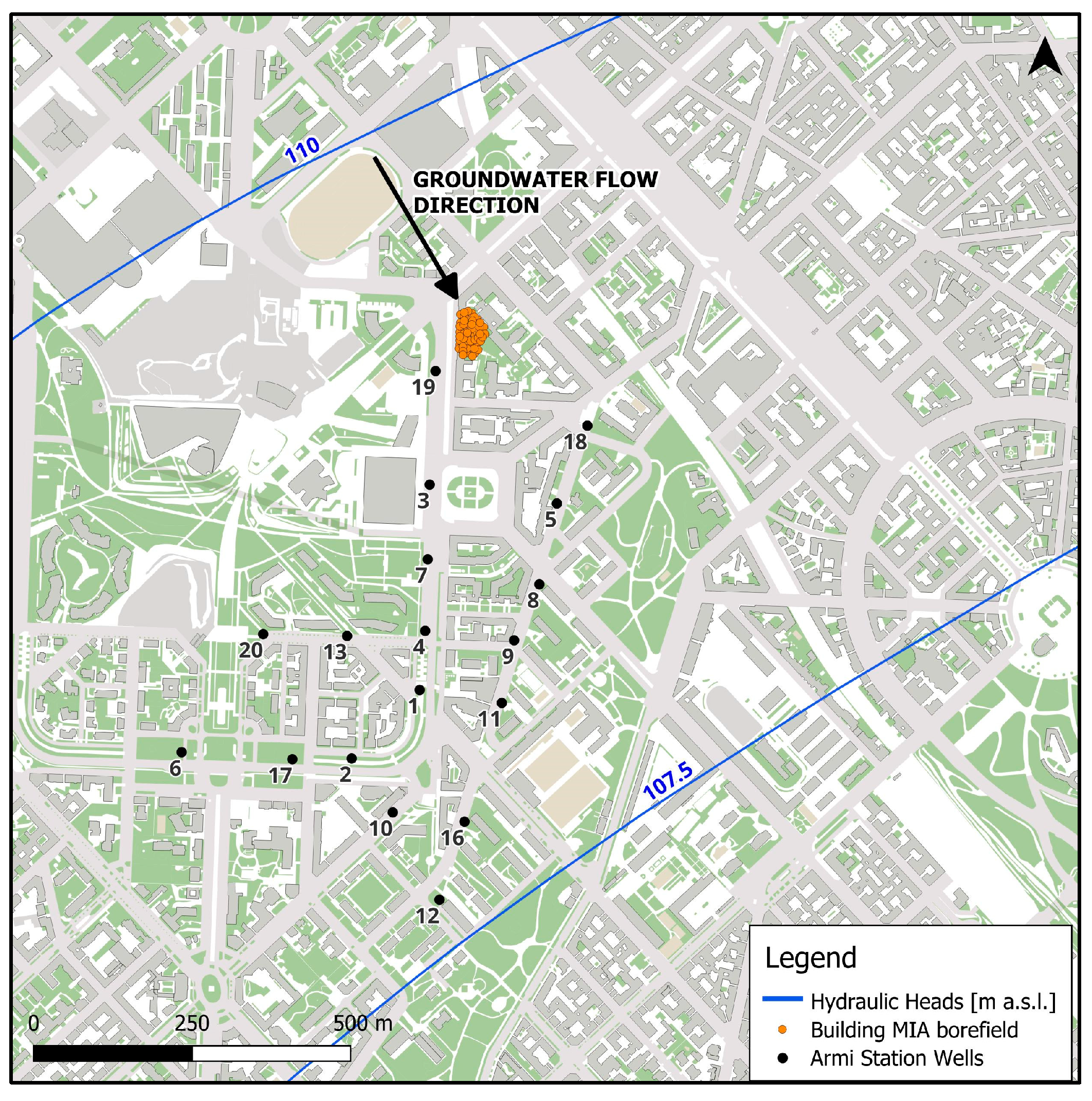
2. The Study Area
3. Materials and Methods
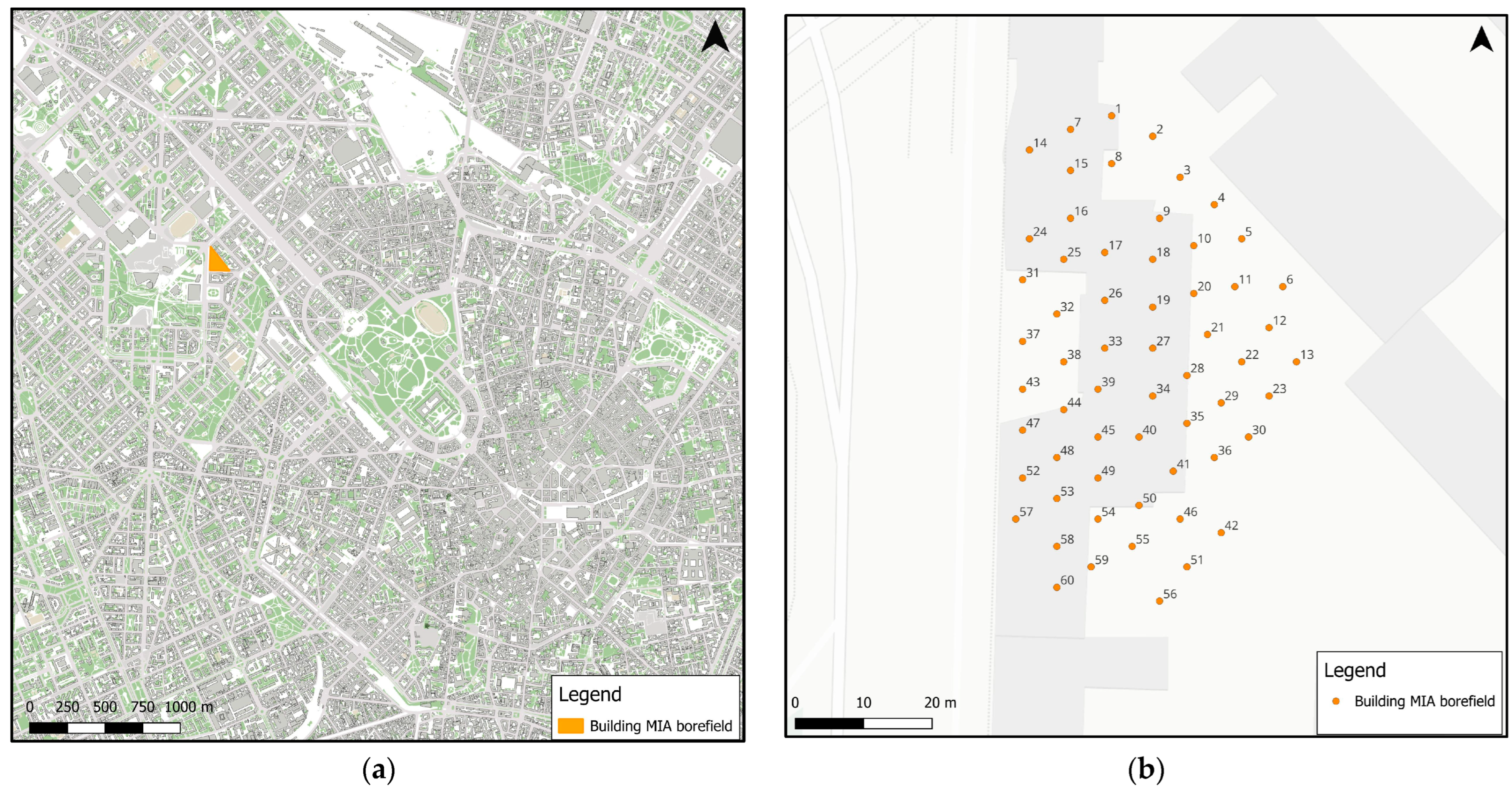
3.1. Building “MIA—La Casa Italiana”
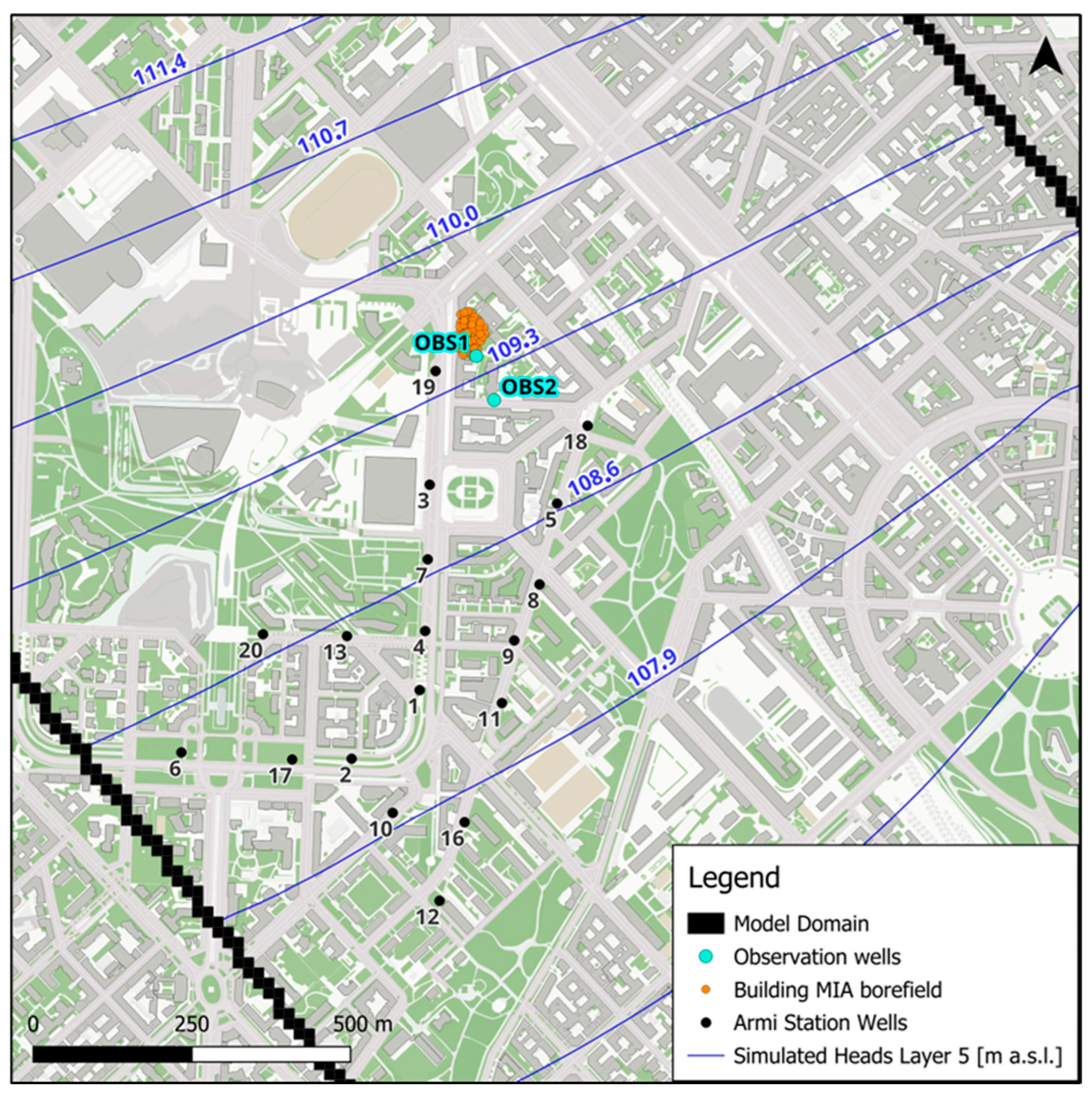
3.2. Numerical Model Implementation
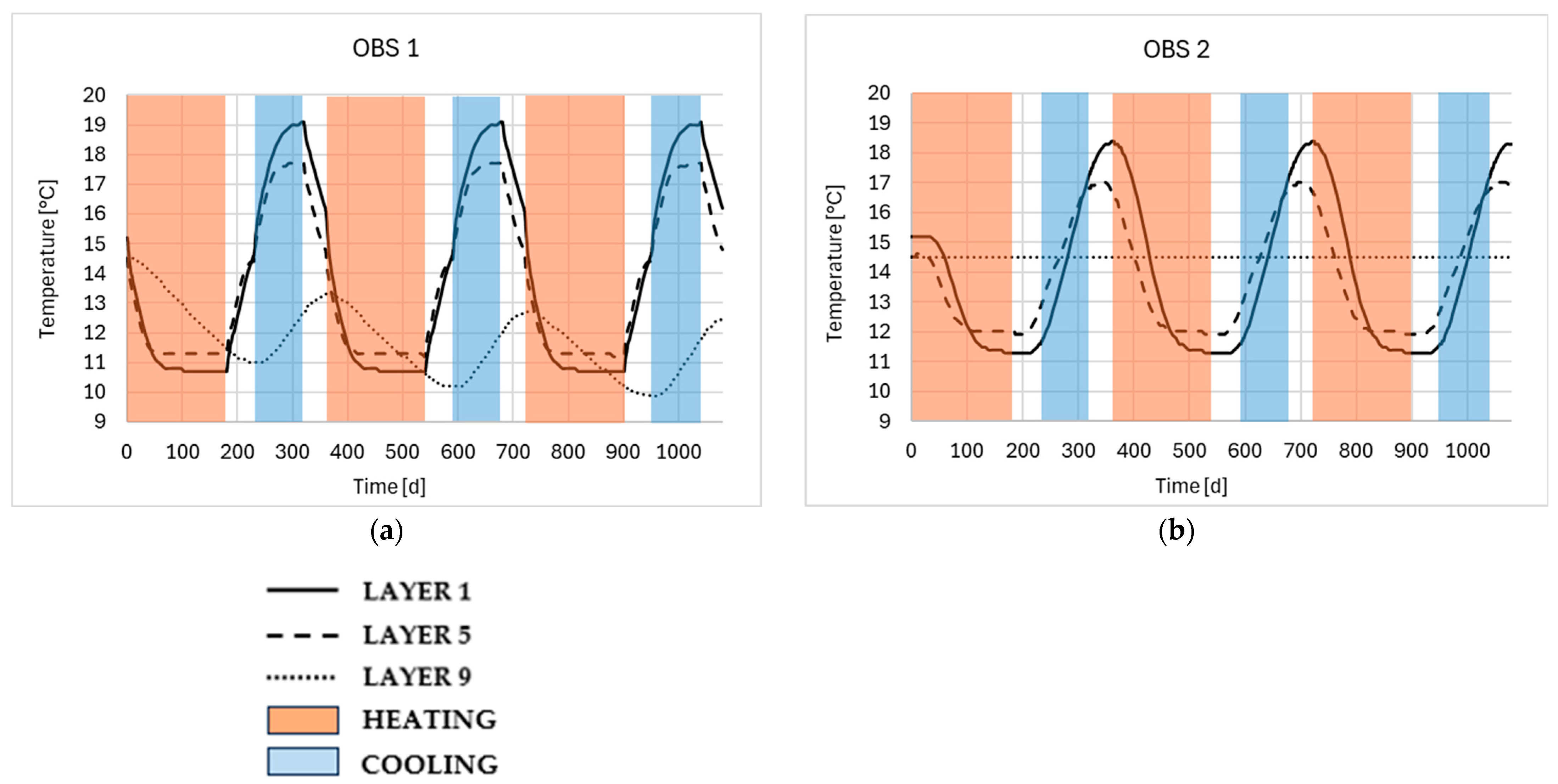
4. Results and Discussion
5. Conclusions
Supplementary Materials
Author Contributions
Funding
Data Availability Statement
Conflicts of Interest
Abbreviations
| CLN | Connected linear network |
| BHEs | Borehole heat exchangers |
| GSHP | Ground-source heat pump |
| GWHP | Groundwater heat pump |
| UHI | Urban heat island |
| TMR | Telescopic mesh refinement |
| CVFD | Control volume finite difference |
| TRT | Thermal response test |
References
- Lund, J.W.; Boyd, T.L. Direct Utilization of Geothermal Energy 2015 Worldwide Review. Geothermics 2016, 60, 66–93. [Google Scholar] [CrossRef]
- Alberti, L.; Angelotti, A.; Antelmi, M.; La Licata, I. A Numerical Study on the Impact of Grouting Material on Borehole Heat Exchangers Performance in Aquifers. Energies 2017, 10, 703. [Google Scholar] [CrossRef]
- Alberti, L.; Angelotti, A.; Antelmi, M.; La Licata, I. Borehole Heat Exchangers in Aquifers: Simulation of the Grout Material Impact. Rend. Online Soc. Geol. Ital. 2016, 41, 268–271. [Google Scholar] [CrossRef]
- Angelotti, A.; Alberti, L.; La Licata, I.; Antelmi, M. Borehole Heat Exchangers: Heat Transfer Simulation in the Presence of a Groundwater Flow. J. Phys. Conf. Ser. 2014, 501, 012033. [Google Scholar] [CrossRef]
- Zhu, K.; Bayer, P.; Grathwohl, P.; Blum, P. Groundwater Temperature Evolution in the Subsurface Urban Heat Island of Cologne, Germany. Hydrol. Process. 2015, 29, 965–978. [Google Scholar] [CrossRef]
- Previati, A.; Crosta, G. Impact of Groundwater Flow on Thermal Response Tests in Heterogeneous Geological Settings. Geothermics 2025, 127, 103266. [Google Scholar] [CrossRef]
- Mao, R.; Chen, Y.; Zhang, Z.; Chen, J.; Zhou, J.; Wu, H. Study on Performance and Layout Optimization of Buried Heat Exchangers Array in Karst Landform. Appl. Therm. Eng. 2025, 271, 126307. [Google Scholar] [CrossRef]
- Champagne-Péladeau, L.; Pasquier, P.; Millette, D.; Dupuis, J.C. Delineation of the Thermal Plume Associated with a Standing Column Well System in a Fractured Aquifer Using Numerical Modeling. Geothermics 2025, 127, 103260. [Google Scholar] [CrossRef]
- Alaie, O.; Maddahian, R.; Heidarinejad, G. Investigation of Thermal Interaction between Shallow Boreholes in a GSHE Using the FLS-STRCM Model. Renew. Energy 2021, 175, 1137–1150. [Google Scholar] [CrossRef]
- Piga, B.; Casasso, A.; Pace, F.; Godio, A.; Sethi, R. Thermal Impact Assessment of Groundwater Heat Pumps (GWHPs): Rigorous vs. Simplified Models. Energies 2017, 10, 1385. [Google Scholar] [CrossRef]
- Perego, R.; Dalla Santa, G.; Galgaro, A.; Pera, S. Intensive Thermal Exploitation from Closed and Open Shallow Geothermal Systems at Urban Scale: Unmanaged Conflicts and Potential Synergies. Geothermics 2022, 103, 102417. [Google Scholar] [CrossRef]
- Halilovic, S.; Böttcher, F.; Zosseder, K.; Hamacher, T. Optimization Approaches for the Design and Operation of Open-Loop Shallow Geothermal Systems. Adv. Geosci. 2023, 62, 57–66. [Google Scholar] [CrossRef]
- Cappellari, D.; Piccinini, L.; Pontin, A.; Fabbri, P. Sustainability of an Open-Loop GWHP System in an Italian Alpine Valley. Sustain. 2023, 15, 270. [Google Scholar] [CrossRef]
- Di Dato, M.; D’Angelo, C.; Casasso, A.; Zarlenga, A. The Impact of Porous Medium Heterogeneity on the Thermal Feedback of Open-Loop Shallow Geothermal Systems. J. Hydrol. 2022, 604, 127205. [Google Scholar] [CrossRef]
- Böttcher, F.; Halilovic, S.; Günther, M.; Hamacher, T.; Zosseder, K. Integration of Thermal Groundwater Use in Heat Planning. Grundwasser 2025, 30, 19–35. [Google Scholar] [CrossRef]
- Casasso, A. The Role of Numerical Modelling in the Design of Open-Loop Shallow Geothermal Systems. Rend. Online Soc. Geol. Ital. 2024, 64, 20–25. [Google Scholar] [CrossRef]
- Casasso, A.; Sethi, R. Efficiency of Closed Loop Geothermal Heat Pumps: A Sensitivity Analysis. Renew. Energy 2014, 62, 737–746. [Google Scholar] [CrossRef]
- Criollo, R.; Vilarrasa, V.; Orfila, A.; Marbà, N.; Fernández-Mora, A. Borehole Heat Exchangers in Coastal Areas May Reduce Heatwave Seagrass Loss. Geosci. Lett. 2025, 12, 2. [Google Scholar] [CrossRef]
- Brown, C.S.; Falcone, G. Investigating the Impact of Groundwater Flow on Multi-Lateral, U-Type, Advanced Geothermal Systems. Appl. Therm. Eng. 2025, 271, 126269. [Google Scholar] [CrossRef]
- Ahmadfard, M.; Bernier, M. Simulation of Borehole Thermal Energy Storage (BTES) Systems Using Simplified Methods. J. Energy Storage 2023, 73, 109240. [Google Scholar] [CrossRef]
- Katsifarakis, K.L.; Kontos, Y.N. Analytical Optimization of Vertical Closed-Loop Ground Source Heat Pump Systems. Energies 2025, 18, 163. [Google Scholar] [CrossRef]
- Lund, A.E.D. Performance Analysis of Deep Borehole Heat Exchangers for Decarbonization of Heating Systems. Deep Undergr. Sci. Eng. 2024, 3, 349–357. [Google Scholar] [CrossRef]
- Kahwaji, G.Y.; Capuano, D.; Boudekji, G.; Samaha, M.A. Design and Optimization of Ground-Coupled Refrigeration Heat Exchanger in Dubai: Numerical Approach. Heat Transf. 2024, 53, 1474–1500. [Google Scholar] [CrossRef]
- Gizzi, M.; Hosseinpour, F. Evaluating Outlet Working Fluid’s Temperature by Implementing Closed-Loop Geothermal Systems in Decommissioned Hydrocarbon Wells: The Case Studies of San Benigno and Cinzano Wells. Geoing. Ambient. E Mineraria 2024, 171, 44–50. [Google Scholar] [CrossRef]
- Regione Lombardia. Regolamento Regionale n. 2. In Bollettino Ufficiale Della Regione Lombardia; Comune di Milano: Milan, Italy, 2006. [Google Scholar]
- Berta, A.; Gizzi, M.; Taddia, G.; Lo Russo, S. The Role of Standards and Regulations in the Open-Loop GWHPs Development in Italy: The Case Study of the Lombardy and Piedmont Regions. Renew. Energy 2024, 223, 120016. [Google Scholar] [CrossRef]
- Pandey, U.; Basu, D. Effect of Groundwater Flow on Thermal Performance of SBTES Systems. J. Energy Storage 2023, 74, 109375. [Google Scholar] [CrossRef]
- Krcmar, D.; Kovacs, T.; Molnar, M.; Hodasova, K.; Zatlakovic, M. Estimating Thermal Impact on Groundwater Systems from Heat Pump Technologies: A Simplified Method for High Flow Rates. Hydrology 2023, 10, 225. [Google Scholar] [CrossRef]
- Dong, L.; Luo, Z.; Guo, H.; Cheng, L.; Wang, X.; Zhao, Q. The Impact of Developing a Regional Multiwell Groundwater Heat Pump System on the Geological Environment: A Case Study in Haimen, China. Hydrogeol. J. 2024, 33, 257–277. [Google Scholar] [CrossRef]
- Lund, J.W. Direct Utilization of Geothermal Energy. Energies 2010, 3, 1443–1471. [Google Scholar] [CrossRef]
- Bayer, P.; Attard, G.; Blum, P.; Menberg, K. The Geothermal Potential of Cities. Renew. Sustain. Energy Rev. 2019, 106, 17–30. [Google Scholar] [CrossRef]
- Makasis, N.; Kreitmair, M.J.; Bidarmaghz, A.; Farr, G.J.; Scheidegger, J.M.; Choudhary, R. Impact of Simplifications on Numerical Modelling of the Shallow Subsurface at City-Scale and Implications for Shallow Geothermal Potential. Sci. Total Environ. 2021, 791, 148236. [Google Scholar] [CrossRef]
- Ngarambe, J.; Raj, S.; Yun, G.Y. Subsurface Urban Heat Islands: From Prevalence and Drivers to Implications for Geothermal Energy and a Proposed New Framework Based on Machine Learning. Sustain. Cities Soc. 2025, 120, 106153. [Google Scholar] [CrossRef]
- Worsa-Kozak, M.; Arsen, A. Groundwater Urban Heat Island in Wrocław, Poland. Land 2023, 12, 658. [Google Scholar] [CrossRef]
- Menberg, K.; Bayer, P.; Zosseder, K.; Rumohr, S.; Blum, P. Subsurface Urban Heat Islands in German Cities. Sci. Total Environ. 2013, 442, 123–133. [Google Scholar] [CrossRef] [PubMed]
- Hancock, P.J.; Hunt, R.J.; Boulton, A.J. Preface: Hydrogeoecology, the Interdisciplinary Study of Groundwater Dependent Ecosystems. Hydrogeol. J. 2009, 17, 1–3. [Google Scholar] [CrossRef]
- Hähnlein, S.; Bayer, P.; Ferguson, G.; Blum, P. Sustainability and Policy for the Thermal Use of Shallow Geothermal Energy. Energy Policy 2013, 59, 914–925. [Google Scholar] [CrossRef]
- Alberti, L.; Antelmi, M.; Oberto, G.; La Licata, I.; Mazzon, P. Evaluation of Fresh Groundwater Lens Volume and Its Possible Use in Nauru Island. Water 2022, 14, 3201. [Google Scholar] [CrossRef]
- Lepore, D.; Bucchignani, E.; Montesarchio, M.; Allocca, V.; Coda, S.; Cusano, D.; De Vita, P. Impact Scenarios on Groundwater Availability of Southern Italy by Joint Application of Regional Climate Models (RCMs) and Meteorological Time Series. Sci. Rep. 2024, 14, 20337. [Google Scholar] [CrossRef]
- Alberti, L.; Mazzon, P.; Colombo, L.; Cantone, M.; Antelmi, M.; Marelli, F.; Gattinoni, P. Enhancing Groundwater Resource Management in the Milan Urban Area Through a Robust Stratigraphic Framework and Numerical Modeling. Water 2025, 17, 165. [Google Scholar] [CrossRef]
- Casiraghi, G.; Pedretti, D.; Beretta, G.P.; Cavalca, L.; Varisco, S.; Masetti, M. A Multispecies Reactive Transport Model of Sequential Bioremediation and Pump-and-Treat in a Chloroethenes-Polluted Aquifer. Water. Air. Soil Pollut. 2025, 236, 54. [Google Scholar] [CrossRef]
- Pedretti, D.; Masetti, M.; Beretta, G. Pietro Stochastic Analysis of the Efficiency of Coupled Hydraulic-Physical Barriers to Contain Solute Plumes in Highly Heterogeneous Aquifers. J. Hydrol. 2017, 553, 805–815. [Google Scholar] [CrossRef]
- Antelmi, M.; Mazzon, P.; Höhener, P.; Marchesi, M.; Alberti, L. Evaluation of Mna in a Chlorinated Solvents-Contaminated Aquifer Using Reactive Transport Modeling Coupled with Isotopic Fractionation Analysis. Water 2021, 13, 2945. [Google Scholar] [CrossRef]
- Cusano, D.; Coda, S.; De Vita, P.; Fabbrocino, S.; Fusco, F.; Lepore, D.; Nicodemo, F.; Pizzolante, A.; Tufano, R.; Allocca, V. A Comparison of Methods for Assessing Groundwater Vulnerability in Karst Aquifers: The Case Study of Terminio Mt. Aquifer (Southern Italy). Sustain. Environ. Res. 2023, 33, 42. [Google Scholar] [CrossRef]
- Coda, S.; Tufano, R.; Calcaterra, D.; Colantuono, P.; De Vita, P.; Di Napoli, M.; Guerriero, L.; Allocca, V. Groundwater Flooding Hazard Assessment in a Semi-Urban Aquifer through Probability Modelling of Surrogate Data. J. Hydrol. 2023, 621, 129659. [Google Scholar] [CrossRef]
- Muffels, C.; Panday, S.; Andrews, C.; Tonkin, M.; Spiliotopoulos, A. Simulating Groundwater Interaction with a Surface Water Network Using Connected Linear Networks. Groundwater 2022, 60, 801–807. [Google Scholar] [CrossRef]
- Corti, M.; Ghirlanda, E.; Mainetti, M.; Abbate, A.; De Vita, P.; Calcaterra, D.; Papini, M.; Longoni, L. Evaluation of the Applicability of Sediment Transport Models To Dam Filling Prediction in Different Italian Geological Contexts. Ital. J. Eng. Geol. Environ. 2023, 1, 27–32. [Google Scholar] [CrossRef]
- Gatti, F.; Bonaventura, L.; Menafoglio, A.; Papini, M.; Longoni, L. A Fully Coupled Superficial Runoff and Soil Erosion Basin Scale Model with Efficient Time Stepping. Comput. Geosci. 2023, 177, 105362. [Google Scholar] [CrossRef]
- Antelmi, M.; Alberti, L.; Barbieri, S.; Panday, S. Simulation of Thermal Perturbation in Groundwater Caused by Borehole Heat Exchangers Using an Adapted CLN Package of MODFLOW-USG. J. Hydrol. 2021, 596, 126106. [Google Scholar] [CrossRef]
- Previati, A.; Epting, J.; Crosta, G.B. The Subsurface Urban Heat Island in Milan (Italy)—A Modeling Approach Covering Present and Future Thermal Effects on Groundwater Regimes. Sci. Total Environ. 2022, 810, 152119. [Google Scholar] [CrossRef]
- Tolooiyan, A.; Hemmingway, P. A Preliminary Study of the Effect of Groundwater Flow on the Thermal Front Created by Borehole Heat Exchangers. Int. J. Low-Carbon Technol. 2014, 9, 284–295. [Google Scholar] [CrossRef]
- Dehkordi, S.E.; Schincariol, R.A. Effect of Thermal-Hydrogeological and Borehole Heat Exchanger Properties on Performance and Impact of Vertical Closed-Loop Geothermal Heat Pump Systems. Hydrogeol. J. 2014, 22, 189–203. [Google Scholar] [CrossRef]
- Di Pierdomenico, M.; Taussi, M.; Galgaro, A.; Dalla Santa, G.; Maggini, M.; Renzulli, A. Shallow Geothermal Potential and Numerical Modelling of the Geo-Exchange for a Sustainable Post-Earthquake Building Reconstruction (Potenza River Valley, Marche Region, Central Italy). Geothermics 2024, 119, 102954. [Google Scholar] [CrossRef]
- Soltan Mohammadi, H.; Ringel, L.M.; de Paly, M.; Bayer, P. Sequential Long-Term Optimization of Shallow Geothermal Systems under Descriptive Uncertainty and Dynamic Variation of Heating Demand. Geothermics 2024, 121, 103021. [Google Scholar] [CrossRef]
- Panday, S. USG-Transport Version 1.5.0: The Block-Centered Transport (BCT) Process for MODFLOW-USG; GSI Environment: Irvine, CA, USA, 2020. [Google Scholar]
- Barbieri, S.; Antelmi, M.; Panday, S.; Baratto, M.; Angelotti, A.; Alberti, L. Innovative Numerical Procedure for Simulating Borehole Heat Exchangers Operation and Interpreting Thermal Response Test through MODFLOW-USG Code. J. Hydrol. 2022, 614, 128556. [Google Scholar] [CrossRef]
- Harbaugh, A.W. MODFLOW-2005, The U.S. Geological Survey Modular Ground-Water Model—The Ground-Water Flow Process; Geological Survey Techniques and Methods 6-A16; US Department of the Interior, US Geological Survey: Reston, VA, USA, 2005. [Google Scholar]
- Regione Lombardia. Deliberazione n. XI/3502. In Bollettino Ufficiale Della Regione Lombardia; Comune di Milano: Milan, Italy, 2020; p. 44. [Google Scholar]
- Wagner, V.; Blum, P.; Kübert, M.; Bayer, P. Analytical Approach to Groundwater-Influenced Thermal Response Tests of Grouted Borehole Heat Exchangers. Geothermics 2013, 46, 22–31. [Google Scholar] [CrossRef]
- FascÌ, M.L.; Lazzarotto, A.; Acuna, J.; Claesson, J. Analysis of the Thermal Interference between Ground Source Heat Pump Systems in Dense Neighborhoods. Sci. Technol. Built Environ. 2019, 25, 1069–1080. [Google Scholar] [CrossRef]


| Layer | Thickness [m] | Hydrogeological Unit |
|---|---|---|
| 1 | 30 | Aquifer A |
| 2 | 4 | Aquitard |
| 3 | 4 | Deep aquifer A |
| 4 | 5 | Aquitard |
| 5 | 18 | Aquifers B1and B2 |
| 6 | 5 | Aquitard |
| 7 | 32 | Aquifers B3 and B4 |
| 8 | 12 | Aquitard |
| 9 | 40 | Aquifer C |
| Stress Period | Season | Duration [d] | Inlet Temperature [°C] |
|---|---|---|---|
| 1 | Winter | 180 | 1 |
| 2 | Spring | 50 | - |
| 3 | Summer | 90 | 28 |
| 4 | Autumn | 40 | - |
| Layer | Hydraulic Conductivity [m/s] | Porosity [-] | Darcy Velocity [m/s] |
|---|---|---|---|
| 1 | 2.9 × 10⁻³–3.3 × 10⁻³ | 0.2 | 7.5 × 10⁻⁶ |
| 2 | 1.8 × 10⁻⁶–1.9 × 10⁻⁶ | 0.05 | 4.5 × 10⁻⁹ |
| 3 | 3.4 × 10⁻³–3.8 × 10⁻³ | 0.2 | 8.8 × 10⁻⁶ |
| 4 | 9.4 × 10⁻⁸–9.4 × 10⁻⁸ | 0.05 | 2.3 × 10⁻¹⁰ |
| 5 | 3.3 × 10⁻³–3.7 × 10⁻³ | 0.2 | 8.8 × 10⁻⁶ |
| 6 | 9.4 × 10⁻⁸–9.4 × 10⁻⁸ | 0.05 | 2.3 × 10⁻¹⁰ |
| 7 | 3.3 × 10⁻³–3.7 × 10⁻³ | 0.2 | 8.8 × 10⁻⁶ |
| 8 | 10−8 | 0.05 | 2.5 × 10⁻¹¹ |
| 9 | 5.5 × 10⁻⁵ | 0.2 | 1.4 × 10⁻⁷ |
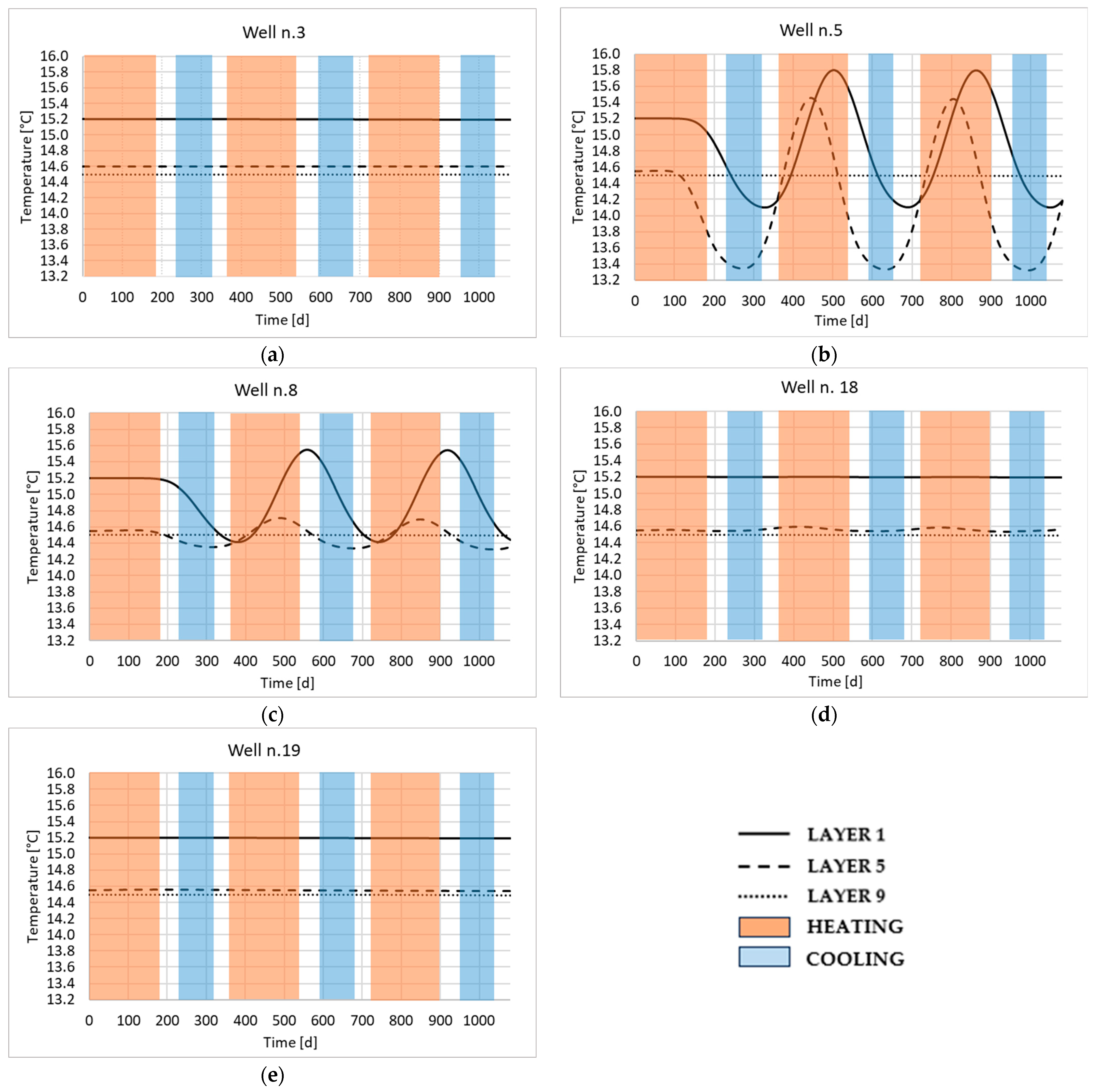
| Time [d] | Period | Layer 1 [°C] | Time [d] | Layer 5 [°C] |
|---|---|---|---|---|
| 328 | Autumn 1st year (stop operation) | −1.10 | 271 | −1.16 |
| 504 | Heating 2nd year | +0.60 | 447 | +0.96 |
| 690 | Autumn 2nd year (stop operation) | −1.10 | 630 | −1.17 |
| 864 | Heating 3rd year | +0.59 | 807 | +0.94 |
| Time [d] | Period | Layer 1 [°C] | Time [d] | Layer 5 [°C] |
|---|---|---|---|---|
| 380 | Heating 2nd year | −0.78 | 311 | −0.15 |
| 557 | Spring 2nd year (stop operation) | +0.35 | 487 | +0.22 |
| 744 | Heating 3rd year | −0.78 | 678 | −0.17 |
| 883 | Heating 3rd year | +0.34 | 847 | +0.30 |
Disclaimer/Publisher’s Note: The statements, opinions and data contained in all publications are solely those of the individual author(s) and contributor(s) and not of MDPI and/or the editor(s). MDPI and/or the editor(s) disclaim responsibility for any injury to people or property resulting from any ideas, methods, instructions or products referred to in the content. |
© 2025 by the authors. Licensee MDPI, Basel, Switzerland. This article is an open access article distributed under the terms and conditions of the Creative Commons Attribution (CC BY) license (https://creativecommons.org/licenses/by/4.0/).
Share and Cite
Barbieri, S.; Antelmi, M.; Mazzon, P.; Rizzo, S.; Alberti, L. Numerical Modeling of the Groundwater Temperature Variation Generated by a Ground-Source Heat Pump System in Milan. Appl. Sci. 2025, 15, 5522. https://doi.org/10.3390/app15105522
Barbieri S, Antelmi M, Mazzon P, Rizzo S, Alberti L. Numerical Modeling of the Groundwater Temperature Variation Generated by a Ground-Source Heat Pump System in Milan. Applied Sciences. 2025; 15(10):5522. https://doi.org/10.3390/app15105522
Chicago/Turabian StyleBarbieri, Sara, Matteo Antelmi, Pietro Mazzon, Sara Rizzo, and Luca Alberti. 2025. "Numerical Modeling of the Groundwater Temperature Variation Generated by a Ground-Source Heat Pump System in Milan" Applied Sciences 15, no. 10: 5522. https://doi.org/10.3390/app15105522
APA StyleBarbieri, S., Antelmi, M., Mazzon, P., Rizzo, S., & Alberti, L. (2025). Numerical Modeling of the Groundwater Temperature Variation Generated by a Ground-Source Heat Pump System in Milan. Applied Sciences, 15(10), 5522. https://doi.org/10.3390/app15105522