
A Hybrid Deep Learning Model Based on FFT-STL Decomposition for Ocean Wave Height Prediction


Abstract
1. Introduction
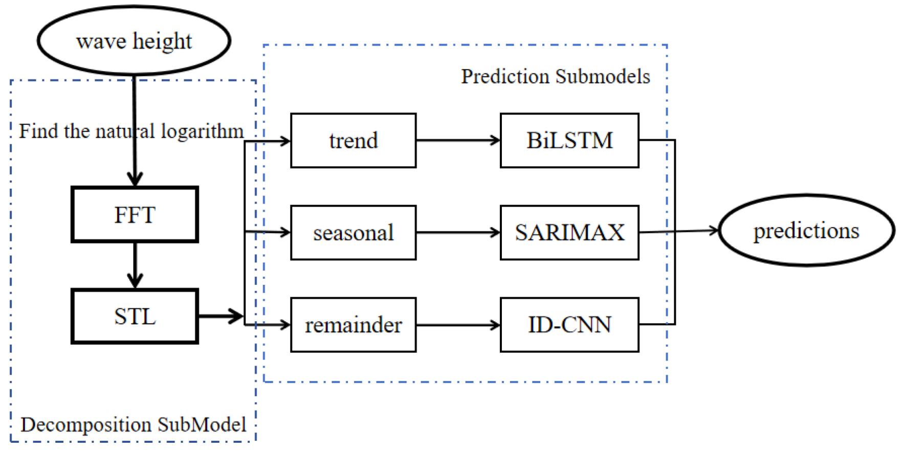
2. Model Design
2.1. Decomposition Submodel
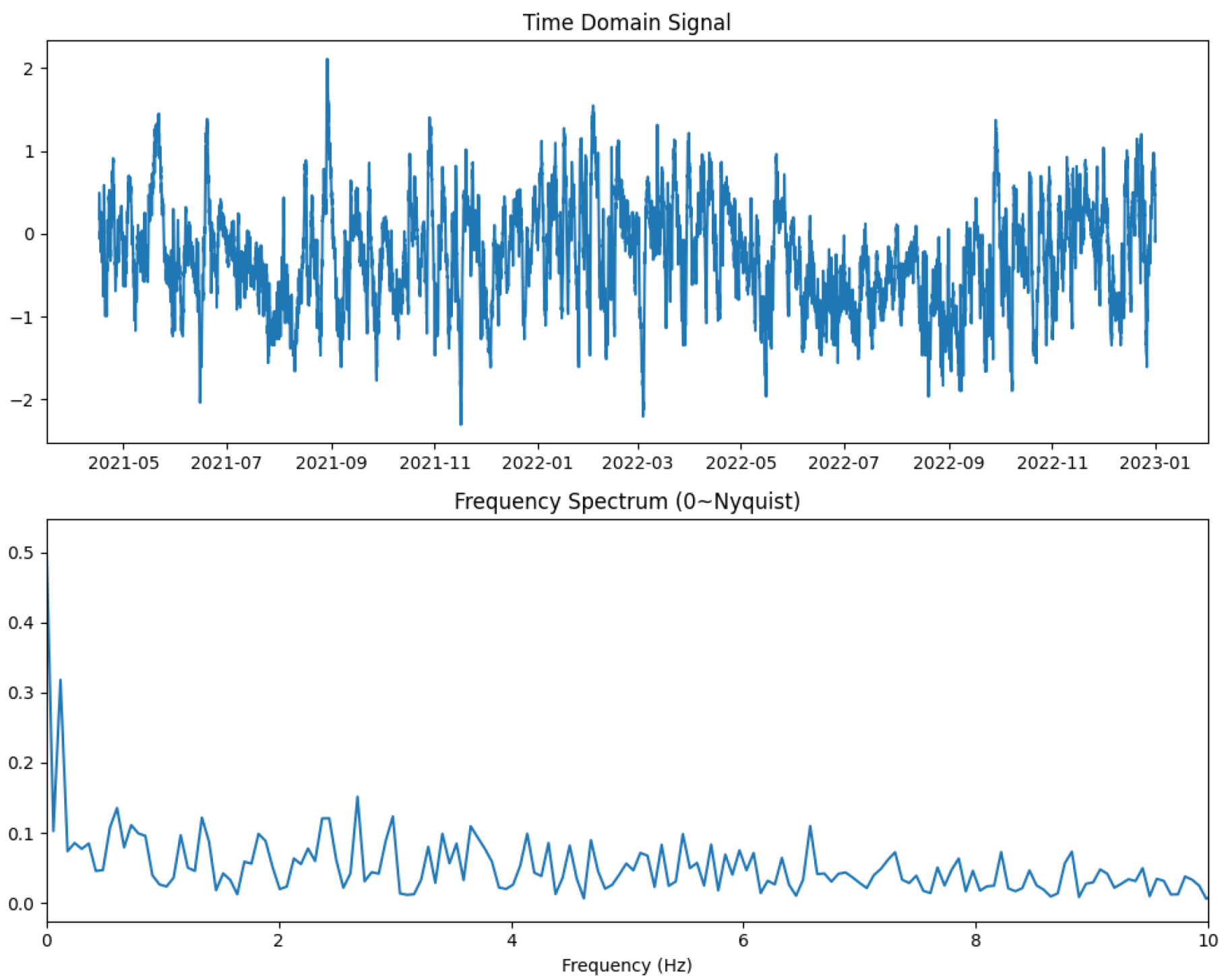
2.1.1. Fast Fourier Transform for Dominant Frequency Extraction
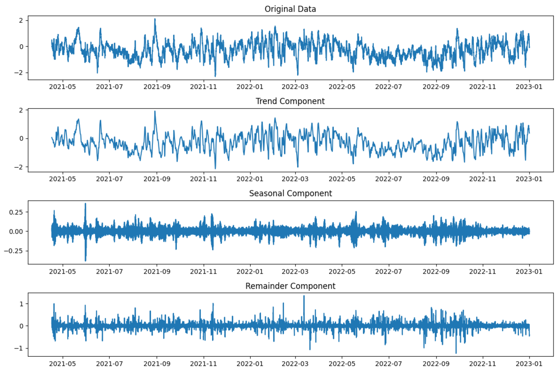
2.1.2. STL for Decomposition
| Algorithm 1: Optimized STL decomposition algorithm. |
 |
2.2. Component-Specific Prediction Submodels
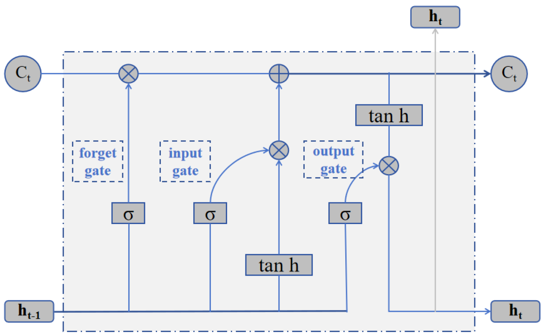
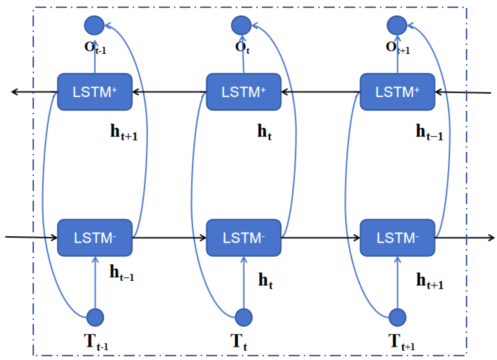
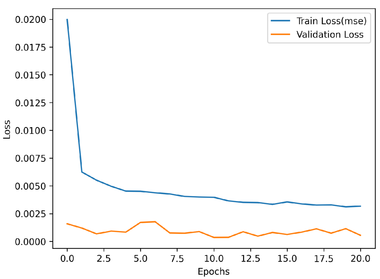
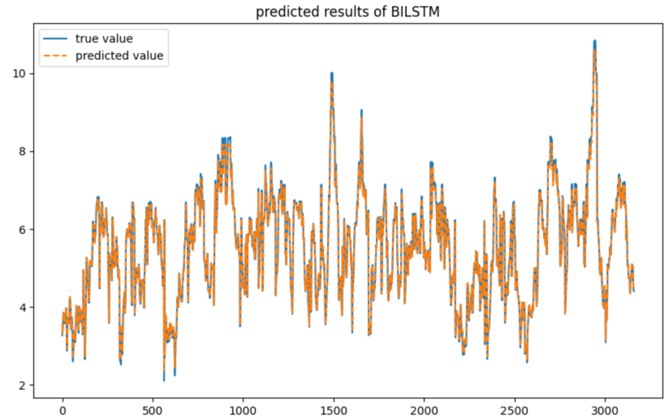
2.2.1. BiLSTM Model for Trend Component Prediction
2.2.2. SARIMAX for Seasonality Component Prediction
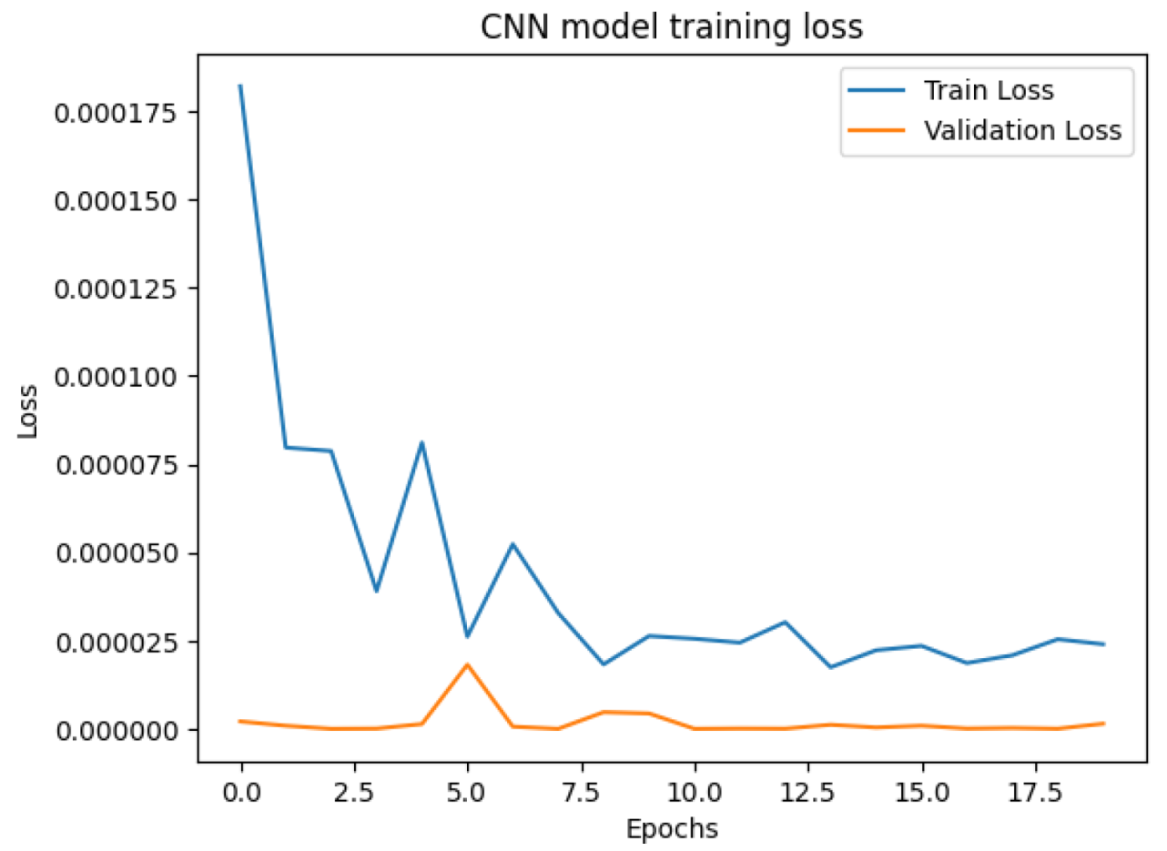
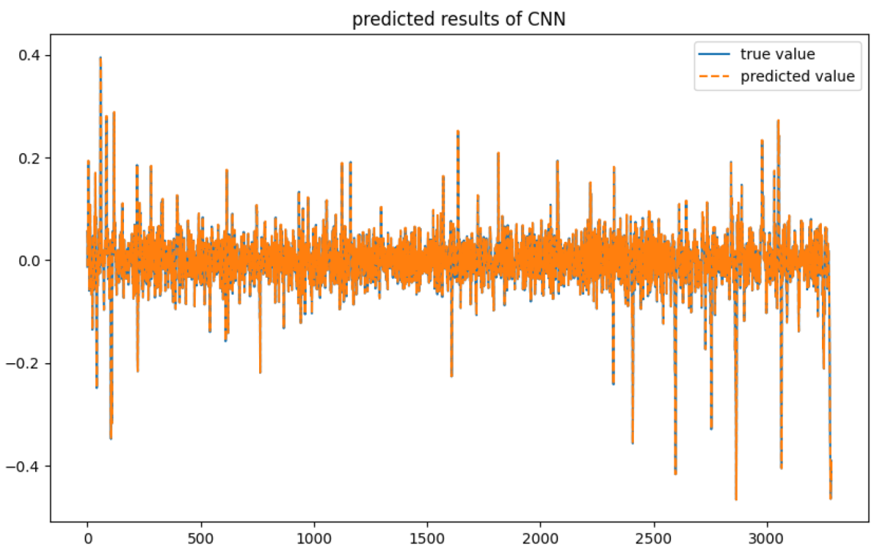
2.2.3. 1D-CNN for Remainder Component Prediction
3. Experimental Results and Analysis
3.1. Datasets
3.2. Evaluation Metrics
3.3. Data Preprocessing
3.4. Data Analysis and Modeling
3.5. Model Comparison
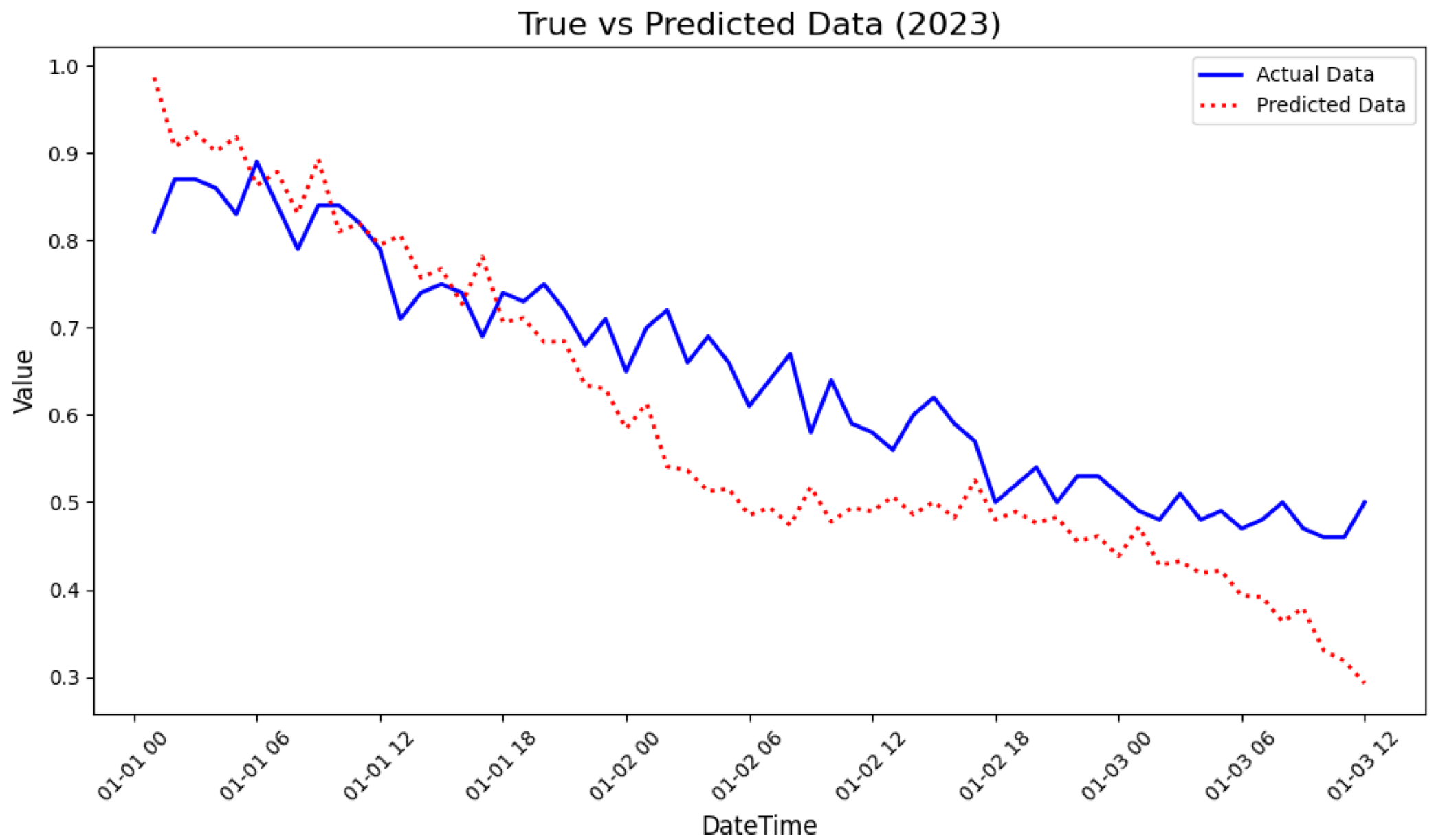
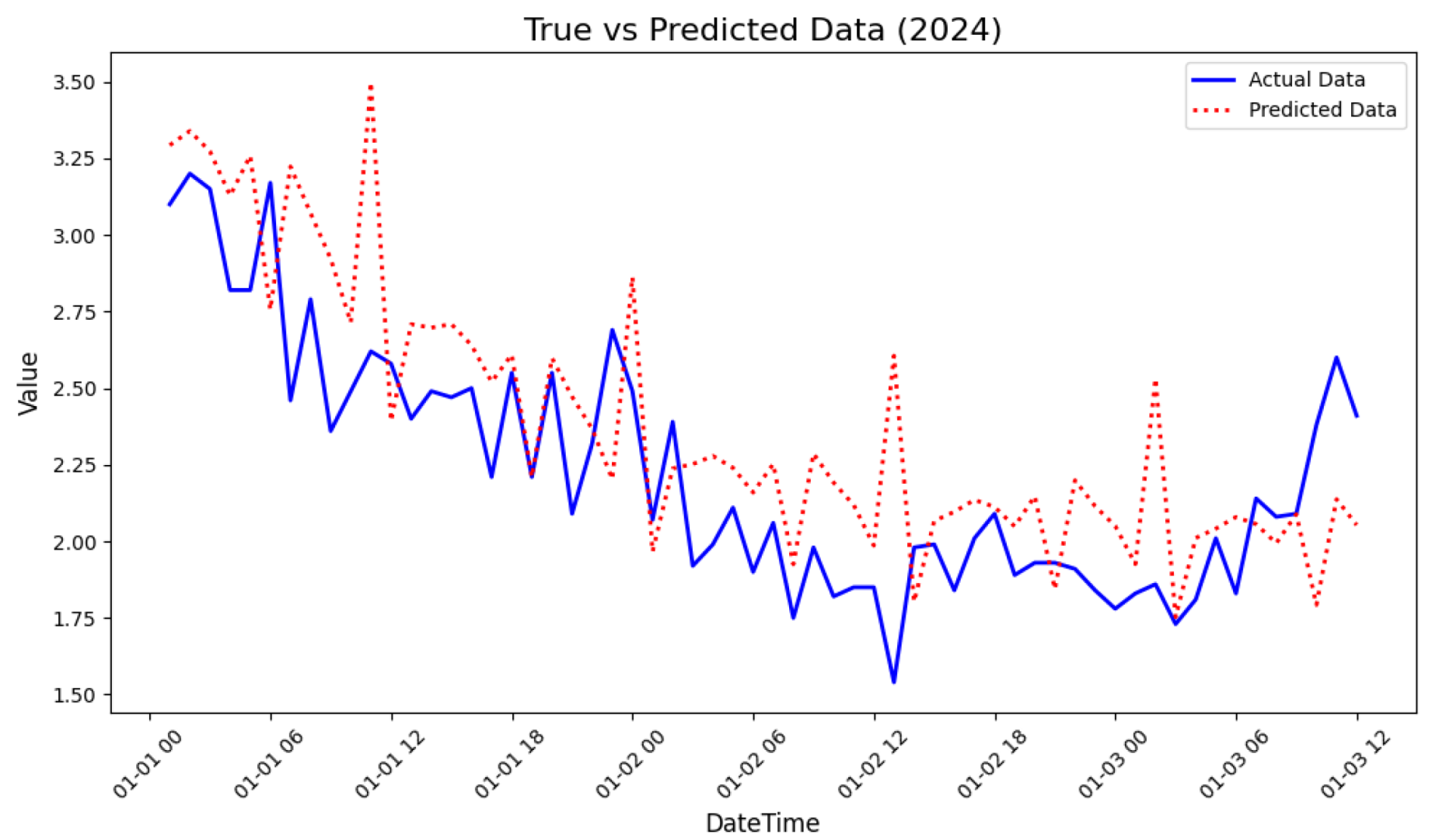
3.6. Prediction About Data
4. Conclusions
Author Contributions
Funding
Data Availability Statement
Conflicts of Interest
Abbreviations
| STL | Seasonal and trend decomposition using Loess |
| AR | Autoregressive |
| SARIMA | Seasonal Autoregressive Integrated Moving Average Model |
| LSTM | Long short-term memory |
| RNNs | Recurrent neural networks |
| 1D-CNN | One-dimensional convolutional neural network |
| BiLSTM | Bidirectional long short-term memory |
| PSD | Power spectral density |
| FFT | Fast Fourier Transform |
| MAE | Mean absolute error |
| RMSE | Root mean square error |
| MAPE | Mean absolute percentage error |
References
- Minuzzi, F.C.; Farina, L. A deep learning approach to predict significant wave height using long short-term memory. Ocean Model. 2023, 181, 102151. [Google Scholar] [CrossRef]
- Ranran, L.; Wang, W.; Li, X.; Zheng, Y.; Lv, Z. Prediction of Ocean Wave Height Suitable for Ship Autopilot. IEEE Trans. Intell. Transp. Syst. 2021, 23, 25557–25566. [Google Scholar]
- Adytia, D.; Saepudin, D.; Pudjaprasetya, S.R.; Husrin, S.; Sopaheluwakan, A. A Deep Learning Approach for Wave Forecasting Based on a Spatially Correlated Wind Feature, with a Case Study in the Java Sea, Indonesia. Fluids 2022, 7, 39. [Google Scholar] [CrossRef]
- Domala, V.; wan Kim, T. Application of Empirical Mode Decomposition and Hodrick Prescot filter for the prediction single step and multistep significant wave height with LSTM. Ocean Eng. 2023, 285, 115229. [Google Scholar] [CrossRef]
- Fu, Y.; Ying, F.; Huang, L.; Liu, Y. Multi-step-ahead significant wave height prediction using a hybrid model based on an innovative two-layer decomposition framework and LSTM. Renew. Energy 2023, 203, 455–472. [Google Scholar] [CrossRef]
- Wei, K.; Hu, K. CFD modeling of orthogonal wave-current interactions in a rectangular numerical wave basin. Adv. Bridge Eng. 2024, 5, 17. [Google Scholar] [CrossRef]
- Zhang, H.; Hu, Y.; Huang, B.; Zhao, X. Verification and validation of a numerical wave tank with momentum source wave generation. Acta Mech. Sin. 2025, 41, 324127. [Google Scholar] [CrossRef]
- Vashist, K.; Singh, K.K. Coupled Rainfall-Runoff and Hydrodynamic Modeling using MIKE + for Flood Simulation. Iran. J. Sci. Technol. Trans. Civ. Eng. 2024. [Google Scholar] [CrossRef]
- Makarynskyy, O. Improving wave predictions with artificial neural networks. Neurocomputing 2004, 31, 709–724. [Google Scholar] [CrossRef]
- Choudhury, J.; Sarkar, B.; Mukherjee, S. Forecasting of engineering manpower through fuzzy associative memory neural network with ARIMA: A comparative study. Neurocomputing 2002, 47, 241–257. [Google Scholar] [CrossRef]
- Yang, S.; Xia, T.; Zhang, Z.; Zheng, C.; Li, X.; Li, H.; Xu, J. Prediction of Significant Wave Heights Based on CS-BP Model in the South China Sea. IEEE Access 2019, 7, 147490–147500. [Google Scholar] [CrossRef]
- Yang, S.; Zhang, Z.; Fan, L.; Xia, T.; Duan, S.; Zheng, C.; Li, X.; Li, H. Long-term prediction of significant wave height based on SARIMA model in the South China Sea and adjacent waters. IEEE Access 2019, 7, 88082–88092. [Google Scholar] [CrossRef]
- Deo, M.; Naidu, C.S. Real time wave forecasting using neural networks. Ocean Eng. 1998, 26, 191–203. [Google Scholar] [CrossRef]
- Sadeghifar, T.; Motlagh, M.N.; Azad, M.T.; Mahdizadeh, M.M. Coastal Wave Height Prediction using Recurrent Neural Networks (RNNs) in the South Caspian Sea. Mar. Geod. 2017, 40, 454–465. [Google Scholar] [CrossRef]
- Van, H.; Mosquera, C.; Nápoles, G. A review on the long short-term memory model. Artif. Intell. Rev. 2020, 53, 5929–5955. [Google Scholar]
- da Silva, M.B.L.; Barreto, F.T.C.; de Oliveira Costa, M.C.; da Silva Junior, C.L.; de Camargo, R. Bias correction of significant wave height with LSTM neural networks. Ocean Eng. 2025, 318, 120015. [Google Scholar] [CrossRef]
- Hu, H.; van der Westhuysen, A.J.; Chu, P.; Fujisaki-Manome, A. Predicting Lake Erie wave heights and periods using XGBoost and LSTM. Ocean Eng. 2021, 164, 101832. [Google Scholar] [CrossRef]
- Reichstein, M.; Camps-Valls, G.; Stevens, B.; Jung, M.; Denzler, J.; Nuno Carvalhais, P. Deep learning and process understanding for data-driven Earth system science. Nature 2019, 566, 195–204. [Google Scholar] [CrossRef]
- Wu, Y.; Wang, J.; Zhang, R.; Wang, X.; Yang, Y.; Zhang, T. RIME-CNN-BiLSTM: A novel optimized hybrid enhanced model for significant wave height prediction in the Gulf of Mexico. Ocean Eng. 2024, 312, 119224. [Google Scholar] [CrossRef]
- Raj, N.; Prakash, R. Assessment and prediction of significant wave height using hybrid CNN-BiLSTM deep learning model for sustainable wave energy in Australia. Sustain. Horiz. 2024, 11, 100098. [Google Scholar] [CrossRef]
- Naeini, S.S.; Snaiki, R. A physics-informed machine learning model for time-dependent wave runup prediction. Ocean Eng. 2024, 295, 116986. [Google Scholar] [CrossRef]
- Su, C.; Liang, J.; He, Z. E-PINN: A fast physics-informed neural network based on explicit time-domain method for dynamic response prediction of nonlinear structures. Eng. Struct. 2024, 321, 118900. [Google Scholar] [CrossRef]
- Chen, C.; Xu, Y.; Zhao, J.; Chen, L.; Xue, Y. Combining random forest and graph wavenet for spatial-temporal data prediction. Intell. Converg. Netw. 2022, 3, 364–377. [Google Scholar] [CrossRef]
- Tan, J.; Li, X.; Zhu, J.; Wang, X.; Ren, X.; Zhao, J. ISP-FESAN: Improving Significant Wave Height Prediction with Feature Engineering and Self-attention Network. Neural Inf. Process. 2023, 1792, 15–27. [Google Scholar]
- Schwarz, K.P.; Sideris, M.G.; Forsberg, R. The use of FFT techniques in physical geodesy. Geophys. J. Int. 1990, 100, 485–514. [Google Scholar] [CrossRef]
- Cleveland, R.B.; Cleveland, W.; McRae, J.; Terpenning, I. STL: A Seasonal-Trend DecompositionProcedure Based on Loess. J. Off. Stat. 1990, 6, 3–73. [Google Scholar]
- Hao, J.; Liu, F. Improving long-term multivariate time series forecasting with a seasonal-trend decomposition-based 2-dimensional temporal convolution dense network. Sci. Rep. 2024, 14, 1689. [Google Scholar] [CrossRef]
- Sareen, K.; Panigrahi, B.K.; Shikhola, T.; Nagdeve, R. An integrated decomposition algorithm based bidirectional LSTM neural network approach for predicting ocean wave height and ocean wave energy. Ocean Eng. 2023, 281, 114852. [Google Scholar] [CrossRef]
- Manigandan, P.; Alam, M.S.; Alharthi, M.; Khan, U.; Alagirisamy, K.; Pachiyappan, D.; Rehman, A. Forecasting Natural Gas Production and Consumption in United States-Evidence from SARIMA and SARIMAX Models. Energies 2021, 14, 6021. [Google Scholar] [CrossRef]


| Model | MSE | RMSE | MAE | Runtime (/epoch) |
|---|---|---|---|---|
| Hybrid-STL model | 0.0087 | 0.0935 | 0.0783 | 24 s |
| BiLSTM | 0.0554 | 0.2353 | 0.1478 | 16.1 s |
| 1D-CNN | 0.0292 | 0.1709 | 0.1534 | 4.2 s |
Disclaimer/Publisher’s Note: The statements, opinions and data contained in all publications are solely those of the individual author(s) and contributor(s) and not of MDPI and/or the editor(s). MDPI and/or the editor(s) disclaim responsibility for any injury to people or property resulting from any ideas, methods, instructions or products referred to in the content. |
© 2025 by the authors. Licensee MDPI, Basel, Switzerland. This article is an open access article distributed under the terms and conditions of the Creative Commons Attribution (CC BY) license (https://creativecommons.org/licenses/by/4.0/).
Share and Cite
Sun, Y.; Yu, L.; Zhu, D. A Hybrid Deep Learning Model Based on FFT-STL Decomposition for Ocean Wave Height Prediction. Appl. Sci. 2025, 15, 5517. https://doi.org/10.3390/app15105517
Sun Y, Yu L, Zhu D. A Hybrid Deep Learning Model Based on FFT-STL Decomposition for Ocean Wave Height Prediction. Applied Sciences. 2025; 15(10):5517. https://doi.org/10.3390/app15105517
Chicago/Turabian StyleSun, Yelian, Longkun Yu, and Dandan Zhu. 2025. "A Hybrid Deep Learning Model Based on FFT-STL Decomposition for Ocean Wave Height Prediction" Applied Sciences 15, no. 10: 5517. https://doi.org/10.3390/app15105517
APA StyleSun, Y., Yu, L., & Zhu, D. (2025). A Hybrid Deep Learning Model Based on FFT-STL Decomposition for Ocean Wave Height Prediction. Applied Sciences, 15(10), 5517. https://doi.org/10.3390/app15105517