Nationwide Adjustment of Unified Geodetic Control Points for the Modernization of South Korea’s Spatial Reference Frame

Abstract

This study presents a nationwide geodetic network adjustment of approximately 5560 unified control points (UCPs) established across South Korea between 2008 and 2021. Addressing the limitations of conventional regional adjustment strategies, the proposed methodology applies a centralized adjustment framework based on the International Terrestrial Reference Frame 2014 (ITRF2014) at epoch 2002.0. Seventeen permanent GNSS stations were rigorously selected and fixed, ensuring spatial uniformity, observational continuity, and metadata consistency. Baseline processing was conducted annually using high-quality GNSS RINEX data, followed by integrated network adjustment with the GAMIT/GLOBK (10.71) software suite. A total of 17,032 observation files were evaluated using an in-house quality control tool (GPS_QC), of which 25.2% failed to meet accuracy thresholds. The final adjustment yielded sub-centimeter precision, with mean residuals of 5.1 ± 0.057 mm (north) and 5.1 ± 0.056 mm (east), and over 99% of results falling within ±3σ. This study confirms the effectiveness of a unified adjustment strategy over conventional region-based approaches and demonstrates its applicability for high-precision national geodetic frameworks. The findings serve as a foundational contribution to the modernization of Korea’s spatial reference system and offer a transferable methodology for other countries pursuing similar geodetic reforms.

1. Introduction

The establishment of a precise and consistent geodetic control network is essential for the advancement of a national spatial data infrastructure. In South Korea, the development of such a network has progressed through distinct historical phases and evolving technological paradigms. Initial efforts during the Japanese colonial period (1910–1945) were largely driven by administrative and military imperatives, resulting in geodetic networks designed for colonial governance [1,2,3,4,5].

Following national liberation in 1945, South Korea confronted severe challenges in rebuilding its geospatial infrastructure, hampered by economic hardship and limited technical capacity. These difficulties were further compounded by the Korean War (1950–1953), which obliterated more than 70% of existing triangulation points and nearly all vertical benchmarks [6].

Systematic modernization of the national geodetic control network began under the leadership of the National Geographic Information Institute (NGII) through two major projects: the First Order Geodetic Network Project (1975–1992) and the Second Order Geodetic Network Project (1986–1994) [6].

Since 2008, in response to the increasing use of global navigation satellite systems (GNSSs), triangulation points—especially those located in remote and mountainous areas—have been systematically relocated to urban regions. This nationwide relocation and modernization initiative is referred to as the unified geodetic control point.

Between 2008 and 2021, approximately 5500 unified geodetic control points (UGCPs) were established across South Korea. Traditionally, each UGCP was computed using observations from a set of four to five nearby satellite reference stations. However, due to inconsistencies in the selection of reference stations across regions, the existing region-based adjustment strategies have proven insufficient in maintaining positional consistency on a national scale.

To overcome this limitation, this study introduces a unified geodetic adjustment strategy that fixes 17 consistent nationwide satellite reference stations as common control points. This approach enables the simultaneous adjustment of all 5500 UGCPs within a single, coherent geodetic network. The proposed strategy is anchored to the International Terrestrial Reference Frame 2014 (ITRF2014) and is designed to enhance spatial coherence, long-term stability, and global compatibility of the national geodetic infrastructure.

Moreover, incidents such as the 1995 Daegu gas explosion have underscored the critical importance of accurate geospatial information for disaster preparedness and infrastructure safety. This study aims to contribute to the modernization of Korea’s geodetic infrastructure by developing a robust adjustment framework, offering a reproducible model for countries seeking to reform and unify their spatial reference systems [7,8,9].

Comparable initiatives have been implemented in countries such as Japan and Germany. Japan’s GEONET has adopted a unified adjustment strategy to improve nationwide positional consistency. Similarly, Germany’s SAPOS network operates a nationwide system of over 270 GNSS reference stations, where signals are permanently recorded and centrally processed to provide real-time correction data across the country. These international benchmarks further highlight the methodological relevance and global applicability of the proposed Korean framework. This foundation is operationalized through the establishment of unified geodetic control points (UGCPs), as illustrated in Figure 1.

2. Materials and Methods

2.1. GNSS Quality Management

In this study, a standardized quality control (QC) protocol was applied to approximately 17,000 RINEX (receiver independent exchange format) files collected from the unified geodetic control points (UGCPs) across South Korea between 2008 and 2021. The QC procedure was implemented prior to the geodetic network adjustment phase to ensure that only high-quality and reliable observation data were used in subsequent computations.

To maintain consistency and reliability throughout the dataset, a set of key quality indicators was extracted and evaluated for each GNSS observation file. These indicators were carefully selected to assess not only the completeness and temporal continuity of the data but also the signal environment and receiver performance—both of which are essential for achieving accurate and stable geodetic positioning. Low-quality data resulting from signal loss, multipath interference, or equipment malfunction can introduce significant errors during network adjustment. Therefore, early detection and exclusion of such data through a rigorous QC process is a critical step in ensuring the integrity of the adjustment results [10].

Key quality indicators were derived from raw GNSS observation data, including the following:

I.

Total observation time (h),

II.

Data acquisition intervals (dt),

III.

Estimated vs. actual number of observations,

IV.

Multipath effect estimates for L1 and L2 signals (MP₁, MP₂),

V.

Cycle-slip ratios (slps, non_slps, o/slps).

These quality indicators were selected based on international GNSS data standards and methodologies established in previous studies. Beyond fundamental QC metrics, GNSS data assessment can incorporate a range of advanced analytical techniques, including coordinate time series analysis, detection of noise and outliers in carrier-phase and code observations, signal-to-noise ratio (SNR) evaluation, and multipath-effect modeling [11].

To further improve positioning accuracy, precise error modeling is often necessary. This involves applying corrections such as phase center offset (PCO) and phase center variation (PCV), as well as using atmospheric delay models for tropospheric and ionospheric effects [12].

Moreover, software packages such as GAMIT/GLOBK incorporate these corrections to enable precise positioning. They are particularly effective in evaluating the relative positioning accuracy between base stations in network-based processing approaches [13].

Table 1. Summary of GNSS observation quality indicators.

Index	Function
first EPOCH	GNSS observation start time (year/month/day/hour)
last EPOCH	GNSS observation end time (year/month/day/hour)
hrs	Total observation duration [unit: hours]
dt	Data reception interval [unit: seconds]
expt	Estimated total number of observations (elevation angle applied)
have	Actual number of observations
$\mathrm{M}\mathrm{P}\_1$	Average multipath length of L1 signal [unit: m]
$\mathrm{M}\mathrm{P}\_2$	Average multipath length of L2 signal [unit: m]
o/slps	(Actual number of observations)/(number of cycle slips)
slps	Number of cycle slips
non_slps	Percentage of observations without cycle slip [unit: %]

summarizes the QC metrics and their functional descriptions.

In addition to the acquisition rate and multipath criteria applied in this study, global GNSS standards—such as those established by the International GNSS Service (IGS)—offer essential benchmarks for data quality assurance. According to IGS guidelines, GNSS stations are required to maintain a data acquisition rate exceeding 99% to qualify for official registration, underscoring the need for robust equipment and minimal signal obstructions [14,15]. Stations exhibiting data loss greater than 1% may be disqualified from registration, emphasizing the importance of maintaining a well-optimized antenna environment and consistently reliable instrumentation.

Multipath effects, represented by MP₁ and MP₂ values, arise when GNSS signals are reflected off surrounding surfaces, leading to interference with the direct signal path. Minimizing multipath effects requires careful selection of installation sites, the use of high-quality antennas, and appropriate receiver configurations that support multipath mitigation features [16,17].

Cycle slips, which represent discontinuities in carrier-phase tracking, can significantly degrade positioning accuracy. IGS recommends limiting cycle slips to fewer than 1 per 1000 observations, a guideline supported by early foundational work [18]. As cycle slips are among the most critical factors affecting the integrity of GNSS measurements, effective detection and removal are essential in the preprocessing stage.

To address this, various quality control tools and algorithms have been developed. For example, Blewitt (1990) [19] introduced the TurboEdit algorithm, which automatically identifies and eliminates outliers and cycle slips from GNSS data. More recent advancements include a window-based QC tool that allows for the evaluation of multipath, signal delays, and data gaps [20]. In this study, we employed PyRINEX, an open-source Python (3.12) package designed to streamline the QC process by automating the detection and classification of low-quality GNSS data [21].

To automate the quality control (QC) process, this study employed the open-source PyRINEX package, applying standardized thresholds tailored to the characteristics of the observation network. These thresholds—acquisition rate ≥ 70%, multipath noise ≤ 0.5 m, and cycle slip ≤ 400—were determined through empirical analysis of over 17,000 RINEX files. Unlike continuously operating IGS stations, the control points in this study are monitored intermittently (typically once every 2 to 3 years for 4 to 8 h per session), justifying the adoption of relaxed QC thresholds.

While tools like TEQC are widely used for GNSS data validation, they do not define fixed cutoff values for quality metrics. Therefore, an internal calibration approach was necessary to establish meaningful thresholds that balance data quality and observational constraints [22,23,24].

Table 2. RINEX file QC analysis (data acquisition rate and cycle slip).

Satellite	Total Observations	Acquisitions	Acquisition Rate	Threshold	Cycle Slip	Comparison
G02	141	19	13.5%	70%	0	unpassed
G03	522	481	92.1%	70%	0	passed
G04	374	274	73.3%	70%	0	passed
…	…	…	…	…	…	…
G06	448	405	90.4%	70%	1	passed
G07	594	473	79.6%	70%	2	unpassed

illustrates sample file classification based on acquisition rate and cycle slips, while

Table 3. RINEX file QC analysis (multipath).

Satellite	MP1	MP2	Comparison
G02	0.41(m)	0.45(m)	passed
G03	0.31	0.41	passed
G04	0.26	0.40	passed
…	…	…	…
G06	0.47	0.74	unpassed
G07	0.40	0.49	passed

summarizes corresponding multipath statistics derived through the QC workflow.

To evaluate long-term trends in GNSS data integrity, this study conducted a temporal analysis of RINEX files collected over a 14-year period. As shown in

Table 4. Unified control point data quality analysis for RINEX network adjustment.

Year	08	09	10	11	12	13	14
Observation point	886	1407	820	23	2396	3382	1089
Outlier	48	61	208	1	604	554	422
Rate	5.4%	4.3%	25.3%	4.3%	25.1%	16.4%	38.8%
Year	15	16	17	18	19	20	21
Observation point	488	647	1941	1770	774	741	668
Outlier	23	188	923	251	370	328	319
Rate	29.1%	29.1%	47.6%	14.1%	47.8%	44.2%	47.2%

, although the number of observation points steadily increased, the proportion of outlier data rose sharply after 2014, exceeding 40% in the years 2020–2021.

This degradation is primarily attributed to a shift in operational practice in South Korea, where GNSS observation sessions have increasingly been conducted for less than 4 h, rather than the previously common 8 h standard. The shortened observation duration likely contributed to a higher incidence of incomplete or low-quality data.

Previous studies have emphasized that robust GNSS data quality assessment is essential for ensuring the reliability of positioning and ionospheric modeling [25]. In particular, systems with low-duty cycles or suboptimal installation environments tend to experience increased cycle slips and multipath errors, while core quality metrics such as signal acquisition rate and satellite geometry may progressively deteriorate over time [26,27].

In summary, the proposed QC framework served as a rigorous data-screening mechanism, allowing only high-integrity GNSS observations to be included in the national geodetic adjustment. This process effectively minimized the propagation of errors from low-quality data and contributed to improving the overall accuracy, consistency, and long-term stability of the unified coordinate system [28].

2.2. GNSS Double-Differenced

In carrier-phase observations, a GNSS receiver measures the phase difference between the incoming satellite signal and its internally generated signal. While the fractional component of the phase can be measured with high precision, the total number of full wavelengths (denoted as N) between the satellite and the receiver at the initial epoch (t₀) remains unknown. This unknown integer is referred to as the carrier phase ambiguity, or integer ambiguity. If no signal interruption occurs, the ambiguity remains constant over time and is referred to as the baseline phase uncertainty (BPU) [13,29].

The carrier-phase observation model is expressed as follows:

$$\mathsf{\Phi }={\displaystyle \frac{\mathsf{\lambda }}{\mathrm{R}}}+\mathrm{N}+\mathsf{\epsilon }$$

(1)

Φ is the observed phase (in cycles),

R is the geometric distance between the satellite and the receiver,

λ is the carrier wavelength,

N is the unknown integer ambiguity, ε is measurement noise or error.

Carrier-phase measurements provide extremely high precision, often exceeding 0.01 cycles, which translates to millimeter-level positional accuracy. When two receivers simultaneously observe the same satellite, their observations are physically correlated due to shared propagation paths. However, in processing, this correlation is typically modeled mathematically using differencing techniques [12].

Assuming that the phase error ε follows a normal distribution with a mean of 0 and a variance of σ², and that the observations are linear and uncorrelated, the variance–covariance matrix of the raw phase observations becomes

$${\mathrm{Q}}_{\mathsf{\Phi }}={\mathsf{\sigma }}^2\cdot \mathrm{I}$$

(2)

where

Q_Φ is the variance–covariance matrix of phase observations,

I is the identity matrix.

GNSS positioning can be performed using either absolute (geocentric) or relative techniques. Absolute positioning typically achieves meter-level accuracy and is mainly used in navigation. In contrast, relative positioning—where the position of one receiver is computed with respect to another fixed receiver—can achieve centimeter- or millimeter-level accuracy [11]. Consequently, geodetic control networks are generally established using relative coordinate systems.

To enhance precision and eliminate common-mode errors, differencing techniques are employed as follows:

Single difference (SD): difference in signals from the same satellite received by two receivers,

$$\mathsf{\Delta }\mathsf{\Phi }={\mathsf{\Phi }}_A^j-{\mathsf{\Phi }}_B^j$$

(3)

Double difference (DD): difference in two SDs, typically from two satellites and two receivers,

$$\nabla \mathsf{\Delta }\mathsf{\Phi }=\left({\mathsf{\Phi }}_A^j-{\mathsf{\Phi }}_B^j\right)-\left({\mathsf{\Phi }}_A^k-{\mathsf{\Phi }}_B^k\right)$$

(4)

Triple difference (TD): difference in two DDs over time, often used for cycle-slip detection.

$$\nabla \mathsf{\Delta }\dot{\mathsf{\Phi }}\mathrm{ }=\mathrm{ }\nabla \mathsf{\Delta }\mathsf{\Phi }\left(t_2\right)\mathrm{ }-\mathrm{ }\nabla \mathsf{\Delta }\mathsf{\Phi }\left(t_1\right)$$

(5)

These techniques eliminate receiver and satellite clock errors and mitigate atmospheric effects. Among them, the double-differencing method is most commonly used for high-precision baseline processing in GNSS and serves as a key component in geodetic network adjustments using software such as GAMIT/GLOBK and Bernese (5.2) [10,30,31].

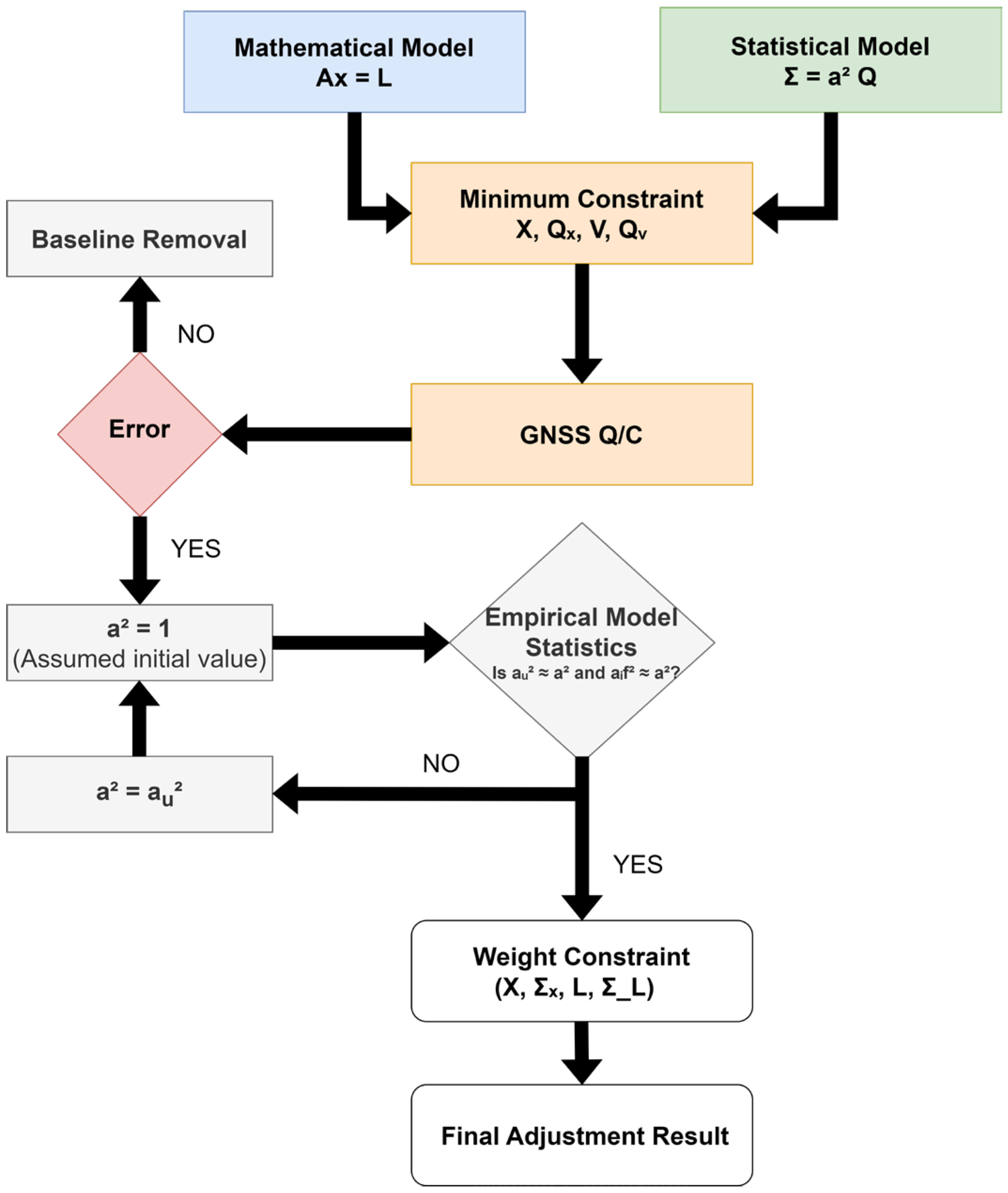
2.3. Network Adjustment Process

Geodetic network adjustment is a fundamental process in geodesy, designed to determine the most probable coordinates of network points by minimizing observational errors. This adjustment ensures that geospatial data maintain high levels of accuracy and reliability, which are essential for applications such as topographic mapping, infrastructure design, and satellite-based navigation systems. The process typically involves constructing mathematical models that relate observations to unknown parameters, and then applying statistical estimation techniques—such as least squares adjustment—to solve and validate these parameters [28,32].

In GNSS-based geodetic networks, the process begins with the establishment of a functional model, A·x = L, and a corresponding stochastic model, Σ = a²·Q. The functional model relates the observation equations to unknowns, while the stochastic model describes the expected behavior of observation errors. Together, these models form the basis for least squares estimation [11,33].

A minimally constrained adjustment is typically applied at the initial stage. This yields preliminary station coordinates (X), variance–covariance matrices (Q_X, Q_V), and observation residuals (V), providing an internal check on the network geometry and data quality [34]. If anomalies or gross errors are found, the adjustment process is refined iteratively.

This iterative refinement does not alter the overall network structure but aims to improve internal consistency by re-evaluating residual patterns and verifying redundancy within the observations. The variance–covariance matrices serve as diagnostic tools, allowing the analyst to assess the relative strength and geometry of the network. In particular, the off-diagonal elements of these matrices offer insight into correlations between parameters, which can indicate potential instability in poorly constrained regions. As illustrated in Figure 2, residuals are also examined not only for magnitude but for systematic trends, as these may point to modeling errors or inconsistencies in observational conditions. Through this process, the adjustment achieves statistical rigor without compromising the spatial integrity of the original network design. The role of variance–covariance matrices in evaluating network strength and parameter interdependence has been extensively discussed in the adjustment literature [35,36,37].

Following model definition, a minimally constrained adjustment is performed to derive initial estimates for station coordinates (X), along with their associated variance–covariance matrices (Q_X, Q_V) and observation residuals (V). Subsequent GNSS quality control (QC) procedures ensure that input observations satisfy predefined accuracy and stability thresholds [38].

Subsequent GNSS quality control (QC) procedures are essential to ensure that observations meet predefined accuracy and stability standards. These include multipath filtering, cycle-slip detection, and statistical outlier analysis using chi-square and F-ratio tests [39,40]. When required, baseline vectors or observations may be excluded, reweighted, or recomputed.

Empirical statistics such as the unit weight variance (a_u²) and iterative factor variance (a_if²) are used to validate the adequacy of the model. If the assumed unit weight variance a² is consistent with the empirical values (i.e., a² ≈ a_u² and a² ≈ a_if²), the stochastic model is considered accurate, and the network solution can be finalized. Otherwise, the adjustment process is repeated with updated variance assumptions, where a² is typically updated using a_u², as it is derived directly from the residuals. The a_if² value is used as a complementary indicator to confirm the convergence and stability of the iterative adjustment process. [15,41].

Modern network adjustments often integrate GNSS vectors with classical terrestrial measurements, such as distances and angles, using rigorous 3D least squares methods. This integration enhances network reliability, particularly in environments with GNSS signal obstructions [42,43]. Adjustment tools like GAMIT/GLOBK and Bernese support these hybrid configurations with flexible weighting schemes and robust error modeling [10,44].

Finally, adherence to international standards such as those of the IGS and NGS ensures the consistency and interoperability of geodetic data across regions [29,45]. By combining rigorous adjustment theory with advanced software and standardized procedures, GNSS network adjustments provide the foundation for precise and sustainable geospatial infrastructure.

2.4. Using GNSS Software

GAMIT (GNSS Analysis at MIT) and GLOBK (Global Kalman Filter) are widely used GNSS processing tools developed at MIT and maintained in collaboration with institutions such as SIO and CfA. Along with GIPSY-OASIS, they support precise positioning, Earth rotation monitoring, and crustal deformation analysis, and are used by organizations like IGS, SOPAC, and UNAVCO [46,47]. Freely available for academic use, GAMIT/GLOBK has been broadly adopted in geodetic research. Essential supporting datasets—such as precise orbits, station coordinates, Earth orientation parameters, and antenna models—are provided by centers like SOPAC to ensure high-accuracy positioning and seamless integration into global reference frames.

GAMIT processes GNSS data using both carrier-phase (L1/L2) and pseudo range code observations. Its baseline analysis primarily uses the ionosphere-free linear combination of dual-frequency carrier-phase data, which effectively eliminates first-order ionospheric errors. Code observations are utilized for initial satellite clock synchronization and phase ambiguity resolution. Observed baseline vectors are estimated using a weighted least squares approach, where the variance in each observation is derived based on its stochastic characteristics [44,47].

GLOBK supports both daily and long-term network adjustments. For daily solutions, the glred module processes individual GAMIT session outputs. For multi-day integration, the globk module combines daily solution files (H-files) using Kalman filtering to estimate consistent station coordinates, velocities, and frame parameters over time. As part of quality control, GLOBK computes chi-square (χ²) statistics for each baseline; those exceeding predefined thresholds (typically χ² > 10) are excluded from the final solution to preserve network statistical integrity [44,47].

The GAMIT/GLOBK processing workflow follows a structured and modular sequence that begins with the formatting of raw GNSS observations and ends with a finalized, statistically validated geodetic network solution. GAMIT modules—such as makej, arc, cfmrg, and solf—perform critical tasks including data preprocessing, modeling of satellite geometry and atmospheric delays, resolution of carrier phase ambiguities, and baseline estimation. Subsequently, GLOBK modules—such as htoglb and glred—integrate these solutions over time, apply robust weighting strategies, and stabilize network parameters through Kalman filtering and reference frame alignment. At each stage, the workflow incorporates automated quality control mechanisms, such as cycle-slip detection, residual analysis, and model misfit diagnostics [13,44,46,47]. Figure 3 illustrates this sequential data flow, emphasizing the systematic design of the software and its emphasis on rigorous statistical filtering to ensure that only high-quality data contribute to the final geodetic solution.

3. Results

3.1. Fixed Point Selection and Baseline Network Diagram

Accurate geodetic network adjustment begins with the careful selection of stable control stations. In this study, ten permanent GNSS stations from the IGS CORE network were chosen to serve as global reference anchors. These stations offer long-term positional stability and are recognized under the ITRF2014 framework, ensuring consistency with international geodetic standards [48,49].

To reinforce the domestic network, seventeen continuously operating reference stations (CORS) within South Korea were selected based on criteria from ICSM (2017) [50] and NGS (2011) [51]:

i.

Continuous and stable GNSS observations suitable for long-term positioning applications.

ii.

No undocumented hardware changes during the adjustment period.

iii.

Complete and validated station metadata including antenna, receiver, and site information.

iv.

Even and appropriate spatial distribution across the national territory.

Stations exhibiting nonlinear motion, incomplete metadata, or known equipment alterations were excluded to avoid introducing regional bias into the adjustment process [52,53].

The resulting set of IGS and domestic CORS ensured both geodetic stability and spatial uniformity across the network.

Figure 4 illustrates the locations of the selected domestic CORS stations.

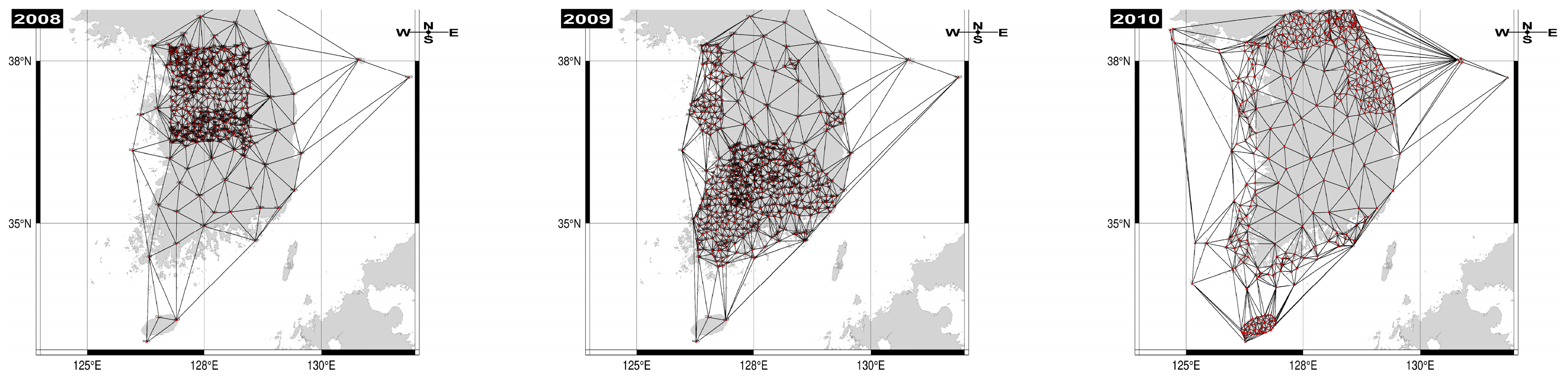
3.2. Pilot Adjustment of Early Unified Control Points (2008–2010) for Strategy Validation

To verify the reliability of the integrated adjustment strategy described in Section 3.1, a pilot adjustment was conducted prior to the nationwide application involving approximately 5560 unified control points (UCPs). This preliminary analysis targeted around 1200 UCPs installed between 2008 and 2010, distributed across diverse regions of South Korea, including Seoul, Gyeonggi, Gangwon, Chungnam, Gyeongsang, Jeolla, and Jeju. The pilot adjustment enabled technical validation of the adjustment methodology and consistency testing against previously published coordinate values.

In the conventional approach, newly installed UCPs were adjusted using short-baseline network processing that connected them to four or five nearby continuously operating reference stations (CORS). The resulting coordinates were published under the Korean Geodetic Datum (KGD), referenced to ITRF2000 at epoch 2002.0.

In contrast, the present study adopts a nationwide strategy using fixed CORS across the entire country and applies a unified adjustment framework referenced to ITRF2014 at epoch 2002.0. This pilot test serves as a reliability assessment for the integrated approach prior to applying the same methodology to all 5560 UCPs in Section 3.3.

Baseline processing and network adjustment were carried out using GAMIT/GLOBK and Bernese software packages, depending on the year of UCP installation. Specifically, GAMIT/GLOBK was applied to UCPs established in 2008 and 2010, while Bernese was used for those installed in 2009. After excluding stations with incomplete observation logs, inconsistent metadata, or poor data quality, the final pilot network consisted of 1193 UCPs. To provide geodetic control, 41 continuously operating reference stations (CORS) were held fixed throughout the adjustment process.

Table 5. Summary of unified control points and adjustment setup for the pilot study.

Year	Region (Example)	Adjustment Software	UCPs
2008	Seoul, Gyeonggi, Gangwon	GAMIT/GLOBK	~300
2009	Gyeongsang, Jeolla	Bernese	~600
2010	Gangwon, Jeju	GAMIT/GLOBK	~300

summarizes the adjustment setup by year, and Figure 5 illustrates the annual distribution of the UCPs used in this pilot study.

The spatial structure of the pilot network and its baseline geometry are shown in Figure 6. The triangulated connections between UCPs demonstrate a dense and uniformly distributed geodetic framework, anchored by fixed CORS across the nation. The resulting baseline network highlights the strong spatial coherence of the integrated adjustment model.

To evaluate the effectiveness of the integrated adjustment strategy, newly computed coordinates were compared with previously published values derived from year-by-year regional adjustments. These earlier adjustments were typically performed independently within localized baseline networks and applied inconsistent stochastic constraints, often aligned with administrative boundaries or observational periods. This fragmented approach resulted in temporal and spatial discontinuities, and over time, such inconsistencies accumulated, leading to systematic distortions within the national geodetic coordinate framework.

In contrast, the integrated adjustment method adopted in this study utilized a unified modeling framework, a consistent set of fixed stations, and harmonized stochastic assumptions across the entire network. This ensured spatial continuity and significantly reduced the influence of regional boundary effects on the final coordinate estimates.

Figure 7 illustrates the frequency distributions of coordinate standard deviations (1σ) for the north, east, and up components, based on the combined dataset over a three-year period. While the figure reveals that more than half of the horizontal deviations (N and E) exceed ±5 mm, this is largely due to the aggregation of all years. A year-by-year analysis reveals more stable results, with a mean deviation of +0.73 mm in the north direction (σ = ±4.65 mm), −1.86 mm in the east direction (σ = ±3.46 mm), and a vertical RMSE of approximately 30.35 mm. The average horizontal RMSE was calculated as 6.13 mm.

These findings not only indicate that residual errors exist in the year-by-year adjustments, but also highlight the spatial distortions and inconsistencies inherent to the regionally segmented adjustment strategy. In contrast, the integrated approach offers improved coordinate precision and spatial consistency, reinforcing the necessity for nationwide adoption to enhance the positional accuracy and geodetic reliability of Korea’s control network.

The consistent magnitude and directional patterns of the differences suggest that the primary source of the discrepancies was not the software used (i.e., GAMIT/GLOBK vs. Bernese), but also the adjustment methodology. Previous regional approaches often applied independent baseline networks and localized constraints, which introduced discontinuities across administrative boundaries and observation years. These inconsistencies accumulated over time, leading to spatial distortions in the official coordinates.

In contrast, the integrated adjustment adopted in this pilot study applied a unified modeling framework, a consistent set of fixed stations, and harmonized stochastic assumptions across the entire network. As a result, the integrated adjustment yielded coherent, homogenous, and statistically robust coordinate estimates.

This pilot evaluation confirms the feasibility and accuracy of the proposed nationwide adjustment strategy. The results strongly support the full-scale implementation of this approach to unify Korea’s spatial reference system, improve geodetic consistency, and enhance the overall reliability of the national control point infrastructure.

In addition to the statistical summaries, spatial visualizations of coordinate differences further illustrate the effectiveness of the integrated adjustment.

Figure 8 displays the horizontal vector differences between the official coordinates derived from previous KGD-based regional adjustments and the results from the integrated adjustment of UCPs installed from 2008 to 2010. The arrows represent both direction and magnitude of positional discrepancies. Clear regional patterns are observed, particularly in areas where independent local adjustments were previously applied, suggesting the accumulation of distortions due to inconsistently defined baselines and constraints.

Figure 9 presents the vertical component of the coordinate differences between the two adjustment strategies. The map reveals substantial variation in ellipsoidal height values, with differences exceeding several decimeters in certain regions. These inconsistencies are primarily attributed to GNSS vertical sensitivity and the absence of leveling-based height control in earlier local adjustments.

These vector-based comparisons provide a compelling visual corroboration of the statistical results presented in

Table 6. Sample results of pilot adjustment and statistical summary of coordinate differences for selected UCPs.

SITE	N	E	H	dN	dE	dH
UCP001	518,199.1056	202,524.8082	69.6456	0.0069	0.0011	−0.0046
UCP002	632,748.5197	300,213.5836	450.1037	−0.0009	0.0027	0.0142
UCP003	649,301.4179	326,825.3849	31.0333	−0.0066	−0.0060	0.0350
UCP004	642,899.4686	327,998.3013	49.0462	−0.0039	−0.0057	0.0404
UCP005	630,251.8133	320,260.1322	610.8182	−0.0048	−0.0068	0.0137
…	…	…	…	…	…	…
			Mean	0.00073	−0.0019	0.0190
			STD	0.0047	0.0035	0.0237
			RMSE	0.0047	0.0039	0.0304
			Max.	0.0123	0.0087	0.4566

, highlighting the extent to which the integrated adjustment strategy mitigates spatial discrepancies. The consistency in vector directions and magnitudes across the network reveals that the unified adjustment not only enhances horizontal positional coherence but also significantly reduces vertical deviations. This integrated approach ensures spatial continuity and eliminates localized distortions introduced by regionally constrained adjustments, thereby reinforcing the robustness and reliability of the national geodetic framework.

Prior to the nationwide adjustment of over 17,000 RINEX datasets, a preliminary test adjustment was conducted using data from the initial three years to evaluate software performance. For this purpose, both GAMIT and Bernese were employed to compare the suitability of each processing strategy. As shown in Figure 8 and Figure 9, notable differences between the two solutions are observed. In the horizontal component, the GAMIT results exhibit systematic residual trends when compared to KGD2002, with deviations largely oriented in a uniform direction. In contrast, the Bernese solution yields smaller residual magnitudes but presents a more scattered directional distribution.

For the vertical component, the GAMIT-derived solution shows minimal differences from KGD2002 in the 2008 dataset, particularly in metropolitan regions such as Seoul, Gyeonggi, and Daejeon. However, larger discrepancies appear in the 2010 dataset, especially in mountainous regions like Gangwon Province. The Bernese results exhibit generally larger vertical discrepancies than GAMIT across all regions and epochs. Based on these comparative findings, GAMIT was selected for the full-scale network adjustment due to its systematic behavior and relatively consistent vertical accuracy.

Further comparative research between GAMIT and Bernese using the full set of 17,000 RINEX files is planned as part of ongoing efforts to assess the long-term performance and consistency of both software platforms in national geodetic applications.

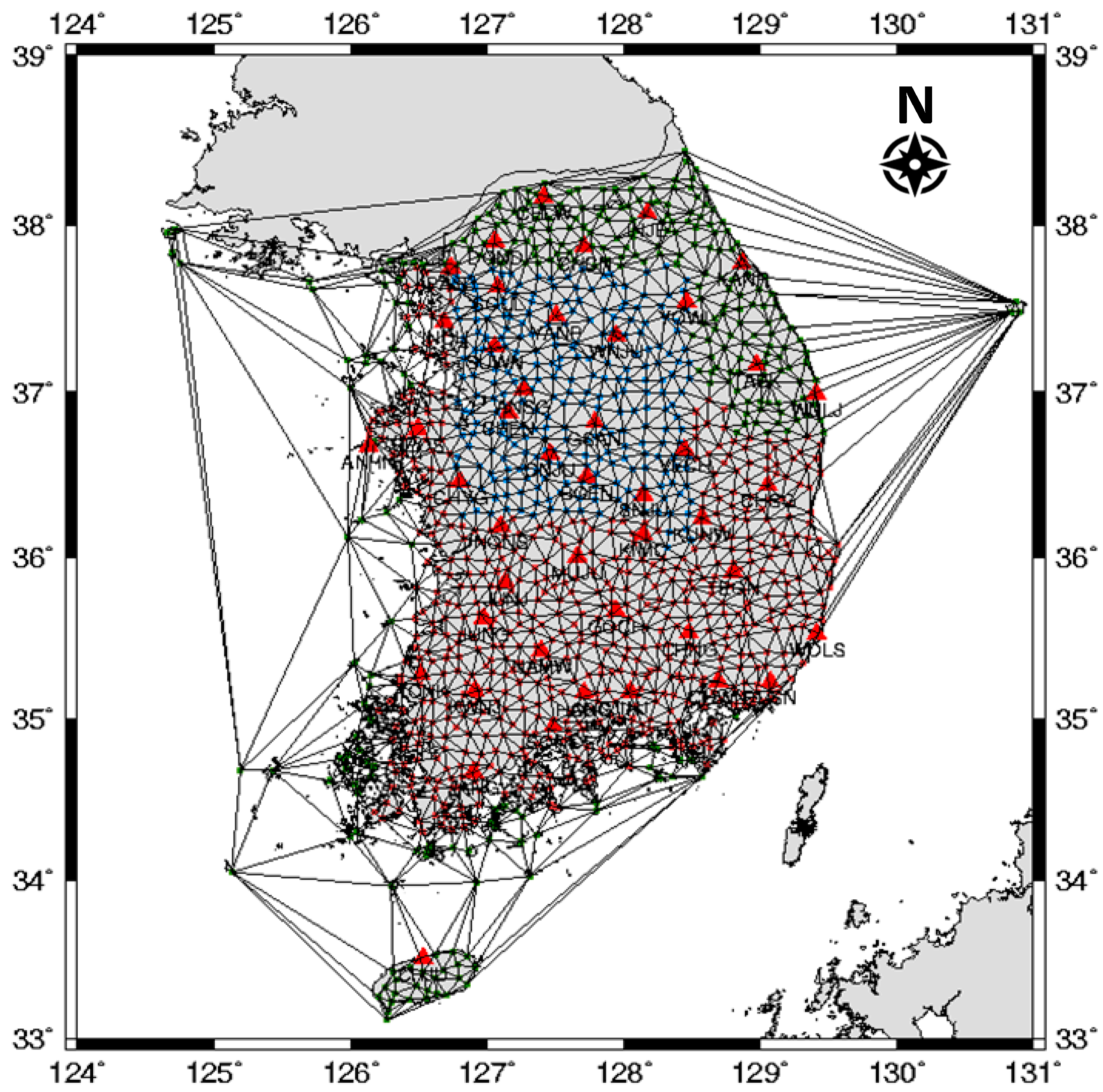
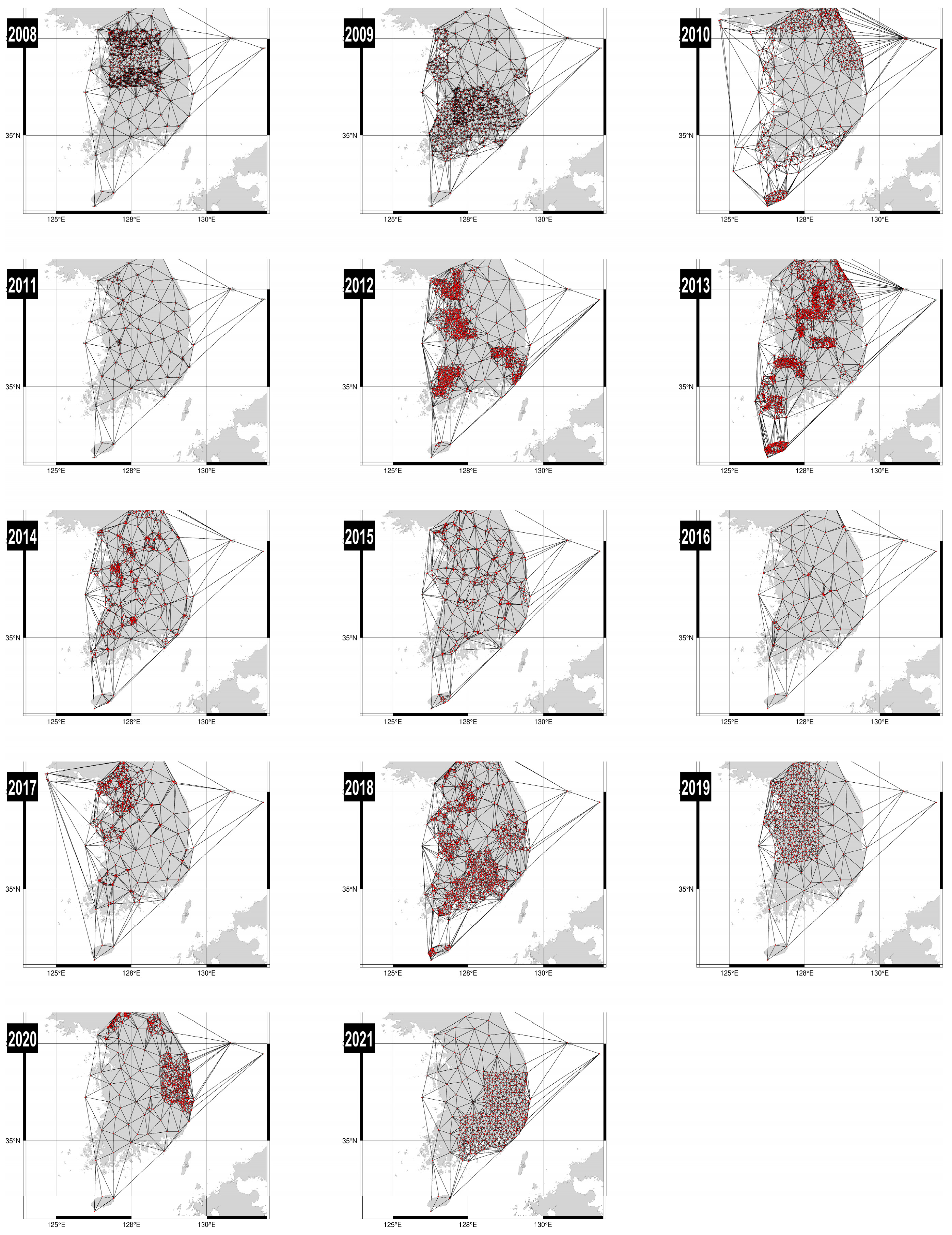
3.3. Full Network Adjustment of 5560 Unified Control Points (2008–2021)

To implement a consistent and accurate adjustment of South Korea’s nationwide unified geodetic control network, approximately 17,000 RINEX files and 17 domestic continuously operating reference stations (CORS) were used to construct a comprehensive geodetic solution. The GNSS observation data spanned the years 2008 to 2021, and baseline processing was performed on a yearly basis to account for variations in installation schedules and field operations.

Unlike previous network adjustment strategies, which relied on four or five locally selected fixed stations per region, the present study adopted a unified adjustment approach using 17 nationally distributed and rigorously verified fixed stations. This strategy—justified by the findings in Section 3.2—ensures superior consistency across space and time, enabling the generation of reliable coordinates free from localized bias or procedural inconsistencies.

Prior to baseline processing, metadata files were prepared to ensure proper modeling of observation geometry and station attributes. The site.apr file defined approximate coordinates for all unified control points (UCPs), while the station.info file included information on observation dates, session durations, antenna types, receiver models, and radome codes. However, inconsistencies were present across the dataset. In many cases, receiver model names were missing, and some stations had incomplete or conflicting metadata. These issues were resolved through manual inspection and correction, with particular reliance on antenna model codes as identifying references.

Significant discrepancies were also found in RINEX file naming conventions. According to national surveying regulations (revised 30 December 2020), observation files should follow the format: SITE (4 characters) + DOY (3 digits) + observation index (1 digit), and contain at least 4 h of continuous data (8 h for pre-2020 data). In practice, however, many sites had inconsistent naming—such as five-character station names or multiple short-duration files per day—resulting from field-level errors. To address this, automated preprocessing procedures were implemented. Station names exceeding four characters were standardized by removing the second character, and DOY values were reassigned based on RINEX header timestamps.

With the dataset corrected and preprocessed, baseline analysis was performed using the GAMIT software for each year from 2008 to 2021. The output H-files served as input for GLOBK, through which the full network adjustment was conducted. The adjustment included all 5560 UCPs, anchored to the 17 fixed stations previously established in Section 3.1, which served as reference coordinates within the ITRF2014 framework.

The spatial distribution of the 5560 UCPs included in the full network adjustment is presented in Figure 10. The map visualizes the nationwide coverage and regional density of the unified control network. It reveals a balanced distribution of control points across both urban and rural areas, ensuring that the adjustment results are geodetically representative of the national territory. The high density of UCPs in the central and southern regions reflects installation priorities in earlier project phases, while peripheral areas such as coastal zones and Jeju Island are also well covered.

This integrated adjustment forms the foundation of a stable and homogeneous national geodetic framework. By applying uniform modeling procedures and a consistent set of reference stations across the entire network, the methodology ensures high positional integrity, comparability of coordinates across time, and alignment with global geodetic standards. It also enhances traceability and enables future reprocessing as part of long-term geodetic infrastructure management.

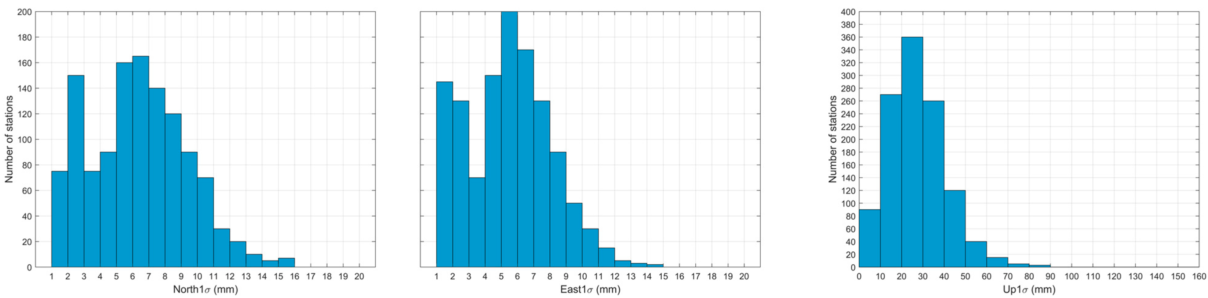
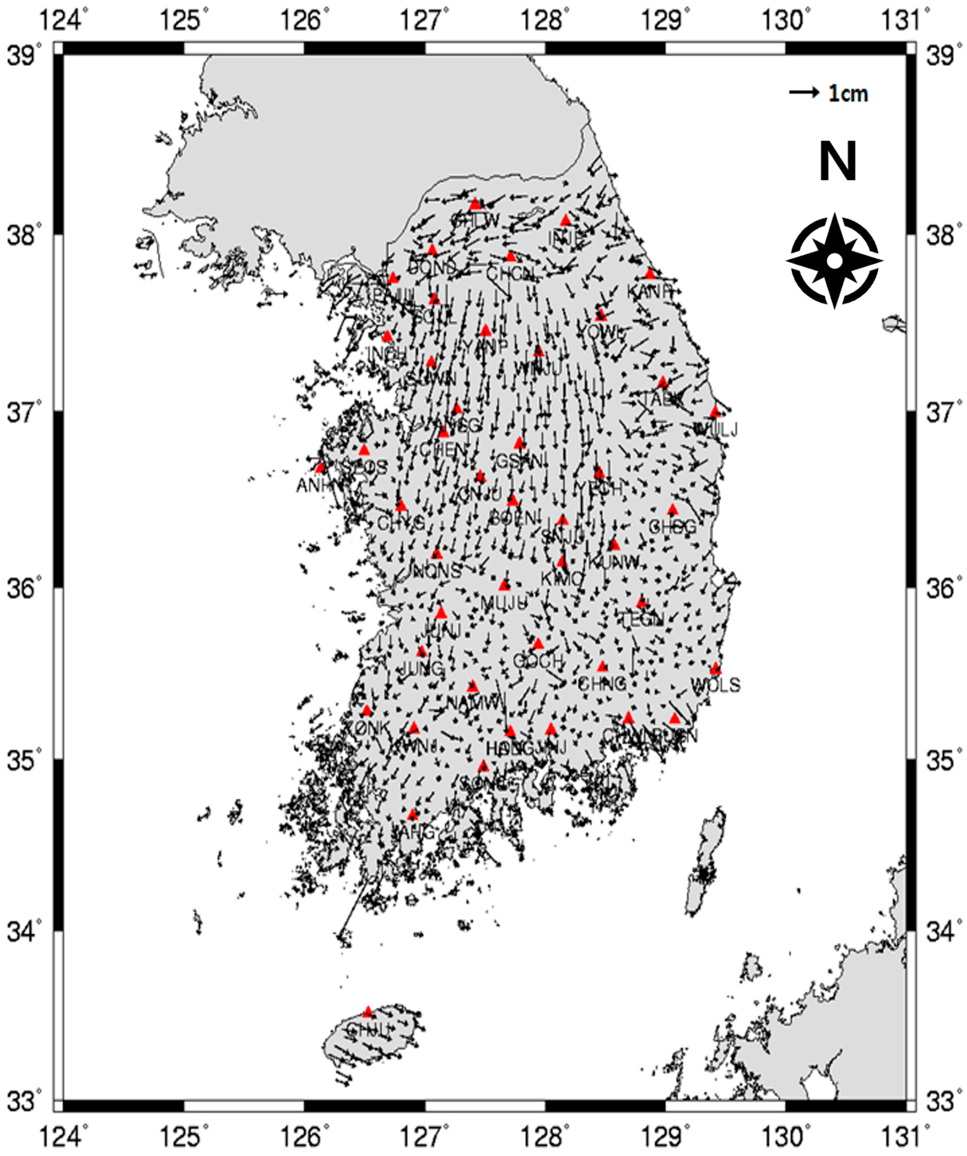
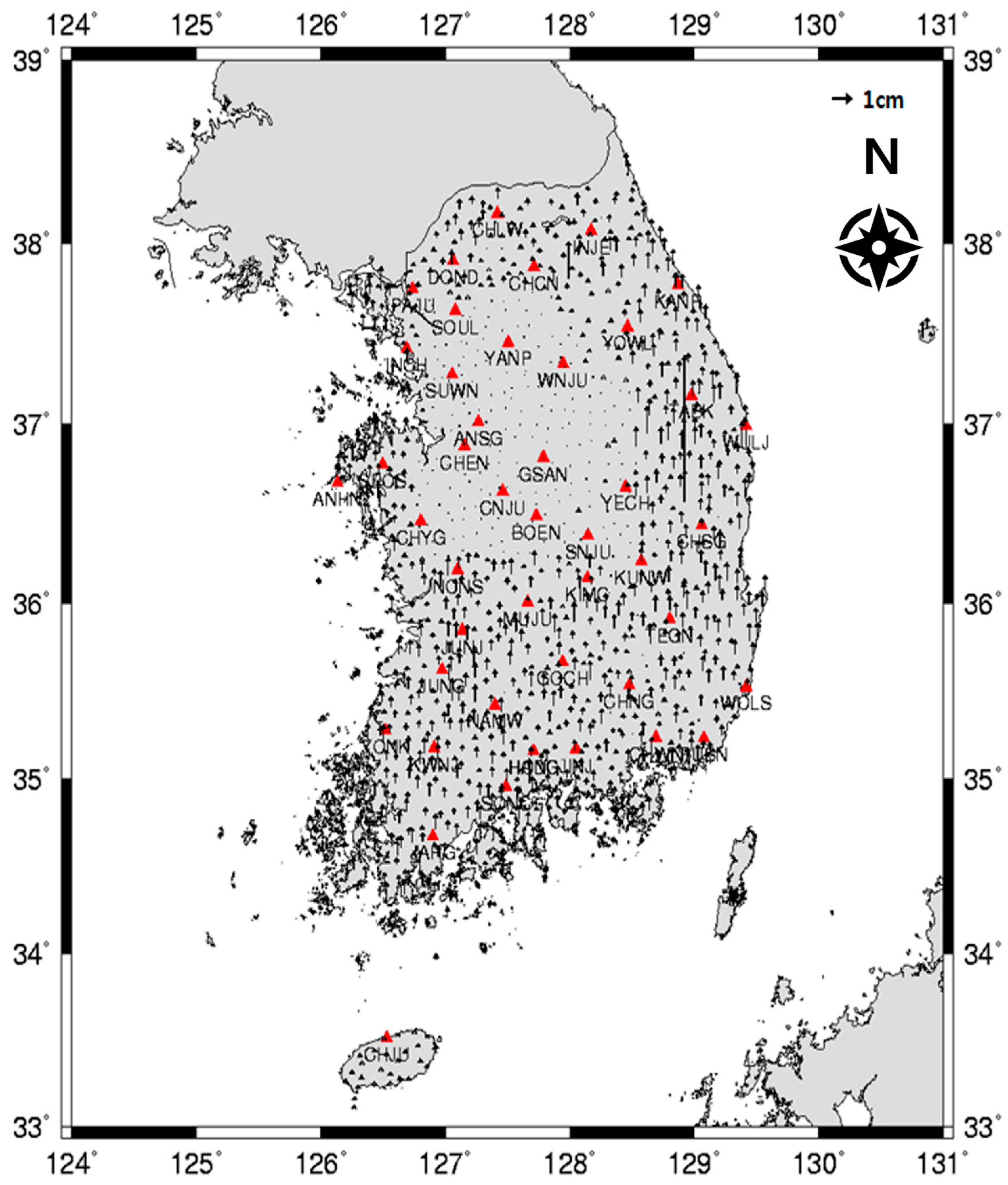
3.4. Accuracy Assessment of GAMIT/GLOBK Adjustment Results

The nationwide geodetic network adjustment was conducted using the GAMIT/GLOBK software suite, referencing the International Terrestrial Reference Frame 2014 (ITRF2014) at the reference epoch of 2002.0. While this epoch coincides with that of Korea’s official geodetic datum (KGD2002), which is aligned with ITRF2000, the present study adopts a more recent and precise realization of the global reference system. All fixed CORS stations were referenced to ITRF2014 coordinates, ensuring enhanced positional consistency aligned with international geodetic standards.

Unlike earlier adjustments in South Korea that employed region-based strategies—typically using four or five locally selected fixed stations per region—this study applied a nationally integrated adjustment framework. By fixing 17 rigorously validated permanent GNSS stations, the adjustment was simultaneously applied to all 5560 UCPs, thereby minimizing regional distortion and supporting homogeneous geodetic control across the entire territory.

To evaluate the precision and internal consistency of the adjustment, residuals in the east (E) and north (N) coordinate components were analyzed. In the east direction, the root mean square error (RMSE) ranged from 0.014 cm to 9.30 cm, with an average of 0.48 cm. The differences between adjusted and previously published coordinates ranged from 0.06 cm to 23.75 cm, with a mean of 0.58 cm. The standard deviation was 0.09 cm, indicating a compact residual distribution consistent with a Gaussian model.

In the north direction, RMSE values ranged from 0.017 cm to 7.20 cm, averaging 0.50 cm. Coordinate differences ranged from 0.02 cm to 60.81 cm, with a mean of 0.56 cm and a standard deviation of 0.093 cm.

Figure 11 shows the histograms of residuals in both directions, overlaid with their respective normal distribution curves. The majority of residuals fall within the ±3σ range, with only 0.16% of north residuals and 0.32% of east residuals exceeding this threshold. This confirms the absence of systematic bias and supports the statistical robustness of the adjustment model.

While a small number of UCPs exhibited deviations exceeding 20 cm, these outliers were primarily attributed to poor GNSS data quality, including incomplete observation sessions, multipath effects, or metadata errors. Such anomalies can be mitigated through preprocessing techniques such as RINEX smoothing, antenna and radome validation, and cycle-slip detection.

A statistical summary of the adjustment results is presented in

Table 7. Summary statistics of coordinate residuals from the GAMIT/GLOBK adjustment, including RMSE, coordinate differences, and standard deviation (E, N, and U directions).

Direction	RMSE (cm)	Coordinate Difference (cm) Min/Max/Mean	Standard Deviation (cm)
East (E)	1.4	0.00/85.69/0.63	1.25
North (N)	1.33	0.00/81.09/0.60	1.18
Vertical (U)	64.8	0/4826.36/3.49	64.71

. The analysis confirms that the unified adjustment framework achieves sub-centimeter RMSE in the horizontal directions while maintaining spatial consistency and statistical reliability across the national geodetic control network. Among the three coordinate components, the vertical direction (up) exhibits the largest root mean square error (RMSE) and standard deviation, which is a well-known limitation of GNSS-based height estimation due to satellite geometry constraints. In contrast, the east and north components show very small standard deviations—1.25 cm and 1.18 cm, respectively—and average residuals below 1 cm. However, all three components include exceptionally large maximum residuals, reaching 85.69 cm (east), 81.09 cm (north), and 4826.36 cm (up). These extreme values are primarily attributed to a small number of control points that were physically relocated during the observation period from 2008 to 2021. The dataset consists of approximately 5500 control stations, observed intermittently every 2 to 3 years. While most stations remained stable and continued to function as part of Korea’s long-term geodetic framework, a few were inevitably reinstalled at nearby locations, leading to significant outliers in both horizontal and vertical components. To minimize the influence of these outliers and to more precisely evaluate the internal consistency of the adjustment, a 3-sigma outlier filtering was applied. The residual distributions in the east, north, and up directions are illustrated in Figure 11.

Table 8. Summary statistics of coordinate residuals from the GAMIT/GLOBK adjustment after applying 3-sigma outlier filtering, including RMSE, coordinate differences, and standard deviation for the east, north, and up directions.

Direction	RMSE (cm)	Coordinate Difference (cm) Min/Max/Mean	Standard Deviation (cm)
East (E)	0.79	0.00/2.48/0.61	0.5
North (N)	50.0	0.00/2.35/0.58	0.48
Vertical (U)	64.8	0.00/9.46/2.35	1.93

presents the coordinate residual statistics after applying a 3-sigma outlier filtering process. The RMSE and standard deviation values for all three components—east, north, and up—are substantially reduced compared to the unfiltered results shown in Table 7. This improvement demonstrates that a small number of extreme residuals had a significant impact on the original statistics. After filtering, the RMSE values were reduced to 0.79 cm (east), 0.50 cm (north), and 1.93 cm (up), with corresponding standard deviations of 0.5 cm, 0.48 cm, and 1.93 cm, respectively. The residual ranges are now tightly constrained, with maximum values not exceeding 2.48 cm (east), 2.35 cm (north), and 9.46 cm (up).

These results emphasize the necessity of establishing a consistent nationwide geodetic framework to eliminate discrepancies and reduce regional deviations that may arise from localized network adjustments. By excluding the influence of extreme outliers, the refined residual statistics demonstrate that a unified adjustment approach can minimize positional inconsistencies across regions and ensure uniform accuracy and internal coherence throughout the national control network. This underscores the importance of adopting a nationwide geodetic adjustment strategy to support high-precision positioning and sustainable geospatial infrastructure management.

4. Discussion

This study proposed and implemented a unified geodetic adjustment strategy for approximately 5560 multi-purpose control points (MPCs) established across South Korea between 2008 and 2021. Departing from previous regionally segmented approaches that relied on localized baseline processing and a limited number of fixed reference stations, the present framework employed 17 rigorously validated continuously operating reference stations (CORS), all referenced to the International Terrestrial Reference Frame 2014 (ITRF2014). This shift toward a nationally integrated adjustment paradigm markedly enhanced spatial uniformity, positional accuracy, and cross-temporal comparability within the national geodetic control network.

The integrated adjustment demonstrated a high degree of internal consistency and coordinate reliability. Mean residuals remained below 1 cm in both east and north directions, and more than 99% of adjusted coordinates fell within ±3σ of the modeled normal distribution, affirming the statistical robustness of the results. Compared to previous region-based adjustments, the unified approach successfully reduced positional discontinuities that had been introduced by inconsistent software versions, adjustment strategies, and fixed station selections across administrative boundaries.

The application of internationally recognized software packages—GAMIT/GLOBK and BERNESE—along with the use of multi-year GNSS observation datasets, enabled the precise modeling of baselines and the generation of repeatable solutions. Rigorous quality control procedures, including antenna and radome verification, receiver metadata validation, and standardization of RINEX file naming and formatting, ensured that systematic errors in input data were minimized throughout the processing pipeline.

Despite these advancements, several limitations remain. A small number of outliers with coordinate residuals exceeding 20 cm were identified. These anomalies were primarily associated with low-quality observation data, inconsistent or missing metadata, or degraded environmental conditions such as severe multipath or signal obstruction. Furthermore, positional degradation was observed in long-baseline segments, particularly in regions with sparse CORS coverage or complex topographic features. These findings highlight the need for future enhancements in stochastic modeling, including the incorporation of baseline length-dependent weighting schemes, and the adoption of advanced preprocessing techniques to further improve data integrity.

Overall, the findings of this study support the adoption of a unified, nationally coordinated adjustment strategy for future control point densification, maintenance, and multi-epoch geodetic applications. The proposed framework offers a scalable, accurate, and repeatable methodology that aligns with international geodetic practices and strengthens the long-term stability of Korea’s national spatial reference system.

5. Conclusions

This study presented a comprehensive nationwide adjustment of South Korea’s unified geodetic control network, encompassing approximately 5560 multi-purpose control points (MPCs) established between 2008 and 2021. A unified adjustment methodology was developed by fixing 17 rigorously validated permanent GNSS stations selected for their long-term observational continuity, antenna stability, and uniform geographic distribution. The adjustment was conducted using annual GNSS observation data within the ITRF2014 reference frame and processed through the GAMIT/GLOBK software suite [44,46,47,53].

Compared to legacy region-based adjustment strategies, the integrated approach significantly improved positional precision and spatial uniformity. The mean coordinate residuals were 5.1 ± 0.057 mm in the northing direction and 5.1 ± 0.056 mm in the easting direction, fulfilling international geodetic accuracy standards [12]. These results validate the feasibility and effectiveness of a centralized adjustment framework for producing high-precision national coordinates.

Satellite geometry, multipath interference, ionospheric delay, and cycle-slip statistics were analyzed. Approximately 25.2% of the datasets failed to meet minimum quality thresholds, underscoring the need for enhanced field acquisition protocols and mandatory quality assurance procedures during national geodetic campaigns.

Although the unified adjustment strategy yielded consistent and reliable results, the study highlights the critical importance of using well-validated and stably maintained control stations throughout the national network. The consistent application of such stations is essential for minimizing regional discrepancies and ensuring positional coherence on a nationwide scale. This concern is supported by recent studies that revealed significant horizontal displacements in long-established control points when proper station validation was lacking, underscoring the practical consequences of insufficient metadata and maintenance [54]. This finding also aligns with the principles established in the development of global reference frames, such as ITRF2000, where the careful selection and long-term stability of reference sites were fundamental to maintaining geodetic integrity across spatial and temporal domains [52]. It further underscores the need to implement a unified framework for station selection and metadata management to support accurate and homogeneous network adjustment.

Looking forward, future research should aim to refine baseline error models, integrate atmospheric and geophysical corrections, and implement fully automated GNSS data quality control systems. Recent developments in artificial intelligence (AI) and machine learning (ML) offer promising opportunities to further enhance adjustment strategies. For instance, Kanhere et al. (2021) [55] proposed a deep neural network model to learn complex GNSS error patterns, while Mohanty and Gao (2022) [56] applied graph convolutional neural networks to predict position corrections. Tang et al. (2024) [57] introduced a reinforcement learning framework for adaptive GNSS adjustment, and Jalalirad et al. (2024) [58] demonstrated improvements in positioning accuracy through graphical neural network-based constellation modeling.

In conclusion, this study proposes a transferable and scalable framework for nationwide high-precision geodetic network adjustment. It enhances the positional accuracy, consistency, and long-term reliability of Korea’s spatial reference infrastructure, while also laying the foundation for future modernization through the convergence of established geodetic techniques and advanced data science methodologies.

References

1. Choi, J.H.; Choi, Y.S. Performance Analysis of the First-Order Geodetic Control Survey in Korea. J. Korean Soc. Surv. Geod. Photogramm. Cartogr. 1994, 12, 15–24. [Google Scholar]
2. Fedman, D. Triangulating Chōsen: Maps, Mapmaking, and the Land Survey in Colonial Korea. Cross-Curr. East Asian Hist. Cult. Rev. 2012, 1, 205–234. [Google Scholar] [CrossRef]
3. Central Intelligence Agency. KOREA: Evaluation of Maps; CIA-RDP79-00976A000100070001-1; Central Intelligence Agency: Washington, DC, USA, 1948. Available online: https://www.cia.gov/readingroom/document/cia-rdp79-00976a000100070001-1 (accessed on 13 April 2025).
4. University of Texas at Austin. Korea Maps—Perry-Castañeda Library Map Collection; University of Texas Libraries: Austin, TX, USA, 1945; Available online: https://maps.lib.utexas.edu/maps/korea.html (accessed on 13 April 2025).
5. National Archives and Records Administration (NARA). Records of U.S. Army Operational, Tactical, and Support Organizations (World War II and Thereafter); Record Group 338; National Archives: Washington, DC, USA. Available online: https://www.archives.gov/research/guide-fed-records/groups/338.html (accessed on 13 April 2025).
6. Choi, J.H.; Choi, Y.S. Simultaneous Adjustment of the Korea Precise Primary Geodetic Network by Development Method. KSCE J. Civ. Environ. Eng. Res. 1993, 13, 151–159. [Google Scholar]
7. Ministry of Land, Infrastructure and Transport (MOLIT). Disaster Management Geospatial Information; MOLIT: Sejong, Republic of Korea, 2020. Available online: https://www.molit.go.kr (accessed on 13 April 2025).
8. Manfré, L.; Santana, R.; Haddad, A.; Campos, M.B.; da Fonseca, L.M.G.; Cartaxo, R. An Analysis of Geospatial Technologies for Risk and Natural Disaster Management. ISPRS Int. J. Geo-Inf. 2012, 1, 166–185. [Google Scholar] [CrossRef]
9. World Bank. The Power of Effective Geospatial Information Management in South Korea: Development and Application; World Bank Group Korea Office: Seoul, Republic of Korea, 2020. Available online: https://documents1.worldbank.org/curated/en/716801606984840817/pdf/The-Power-of-Effective-Geospatial-Information-Management-in-South-Korea-Development-and-Application.pdf (accessed on 13 April 2025).
10. Dach, R.; Lutz, S.; Walser, P.; Fridez, P. (Eds.) Bernese GNSS Software Version 5.2—Documentation; Astronomical Institute, University of Bern: Bern, Switzerland, 2015; Available online: https://www.bernese.unibe.ch/docs/DOCU52.pdf (accessed on 13 April 2025).
11. Leick, A.; Rapoport, L.; Tatarnikov, D. GPS Satellite Surveying, 4th ed.; Wiley: Hoboken, NJ, USA, 2015. [Google Scholar]
12. Teunissen, P.J.G.; Montenbruck, O. (Eds.) Springer Handbook of Global Navigation Satellite Systems; Springer: Cham, Switzerland, 2017. [Google Scholar] [CrossRef]
13. Herring, T.A.; King, R.W.; McClusky, S.C. Introduction to GAMIT/GLOBK; MIT Department of Earth, Atmospheric, and Planetary Sciences: Cambridge, MA, USA, 2018. [Google Scholar]
14. International GNSS Service (IGS). Data Transmission Guidelines; IGS: Bern, Switzerland, 2024; Available online: https://igs.org/data-access/ (accessed on 25 March 2025).
15. Kouba, J. A Guide to Using International GNSS Service (IGS) Products; IGS: Bern, Switzerland, 2009; Available online: http://acc.igs.org/UsingIGSProductsVer21.pdf (accessed on 25 March 2025).
16. Langley, R.B. GPS Receivers and the Observables. In GPS for Geodesy, 2nd ed; Teunissen, P.J.G., Kleusberg, A., Eds.; Springer: Berlin, Heidelberg, 1998; pp. 151–185. [Google Scholar] [CrossRef]
17. Rapiński, J.; Tomaszewski, D.; Pelc-Mieczkowska, R. Analysis of Multipath Changes in the Polish Permanent GNSS Stations Network. Remote Sens. 2024, 16, 1617. [Google Scholar] [CrossRef]
18. Blewitt, G. Carrier phase ambiguity resolution for the Global Positioning System applied to geodetic baselines up to 2000 km. J. Geophys. Res. 1989, 94, 10187–10203. [Google Scholar] [CrossRef]
19. Blewitt, G. An Automatic Editing Algorithm for GPS Data. In IAG Symposia; Springer: Ottawa, ON, Canada, 1990. [Google Scholar] [CrossRef]
20. Lee, D.; Cho, J.; Suh, Y.; Hwang, J.; Yun, H. A New Window-Based Program for Quality Control of GPS Sensing Data. Remote Sens. 2012, 4, 3168–3183. [Google Scholar] [CrossRef]
21. Han, J.; Lee, S.J.; Yun, H.S.; Kim, K.B.; Bae, S.W. PyRINEX: A New Multi-Purpose Python Package for GNSS RINEX Data. PeerJ Comput. Sci. 2024, 10, e1800. [Google Scholar] [CrossRef]
22. Estey, L.H.; Meertens, C.M. TEQC: The Multi-Purpose Toolkit for GPS/GLONASS Data. GPS Solut. 1999, 3, 42–49. [Google Scholar] [CrossRef]
23. Kim, M.; Seo, J.; Lee, J. A Comprehensive Method for GNSS Data Quality Determination to Improve Ionospheric Data Analysis. Sensors 2014, 14, 14971–14993. [Google Scholar] [CrossRef]
24. Lee, J.; Kim, M. Optimized GNSS Station Selection to Support Long-Term Monitoring of Ionospheric Anomalies for Aircraft Landing Systems. IEEE Trans. Aerosp. Electron. Syst. 2017, 53, 236–246. [Google Scholar] [CrossRef]
25. Kowalczyk, K.; Rapiński, J. Robust Network Adjustment of Vertical Movements with GNSS Data. Geofizika 2017, 34, 45–65. [Google Scholar] [CrossRef]
26. Xu, Y.; Ji, S. Data Quality Assessment and the Positioning Performance Analysis of BeiDou in Hong Kong. Surv. Rev. 2015, 47, 446–457. [Google Scholar] [CrossRef]
27. Yigit, C.O.; Gikas, V.; Alçay, S.; Ceylan, A. Performance Evaluation of Short- to Long-Term GPS, GLONASS and GPS/GLONASS Post-Processed PPP. Surv. Rev. 2014, 46, 155–166. [Google Scholar] [CrossRef]
28. Grafarend, E.W. Optimization of geodetic networks. Can. Surv. 1974, 28, 716–723. [Google Scholar] [CrossRef]
29. Kaplan, E.D.; Hegarty, C.J. Understanding GPS: Principles and Applications, 2nd ed.; Artech House: Norwood, MA, USA, 2006. [Google Scholar]
30. Gurtner, W.; Estey, L. The International GNSS Service (IGS): An introduction. In Springer Handbook of Global Navigation Satellite Systems; Teunissen, P.J.G., Montenbruck, O., Eds.; Springer: Cham, Switzerland, 2017; pp. 967–982. [Google Scholar] [CrossRef]
31. Van Hien, N.; Falco, G.; Falletti, E.; Nicola, M.; La, T.V. A Linear Regression Model of the Phase Double Differences to Improve the D3 Spoofing Detection Algorithm. In Proceedings of the 2020 European Navigation Conference (ENC), Dresden, Germany, 23–24 November 2020; pp. 1–14. [Google Scholar] [CrossRef]
32. Xu, G. GPS: Theory, Algorithms and Applications; Springer: Berlin, Germany, 2007. [Google Scholar]
33. Teunissen, P.J.G.; Kleusberg, A. (Eds.) GPS for Geodesy, 2nd ed.; Springer: Berlin, Germany, 1998. [Google Scholar] [CrossRef]
34. Dong, D.; Bock, Y. Global positioning system network analysis with phase ambiguity resolution applied to crustal deformation studies in California. J. Geophys. Res. Solid Earth 1989, 94, 3949–3966. [Google Scholar] [CrossRef]
35. Schaffrin, B. Reliability measures for correlated observations. J. Surv. Eng. 1997, 123, 126–137. [Google Scholar] [CrossRef]
36. Snow, K.B. Notes on Adjustment Computations: Parts I and II; School of Earth Sciences, The Ohio State University: Columbus, OH, USA, 2021; Available online: https://earthsciences.osu.edu/sites/default/files/2021-09/osu_adjustment_computation_notes_parts_1_and_2.pdf (accessed on 15 April 2025).
37. Soler, T.; Marshall, J. Rigorous transformation of variance–covariance matrices of GPS-derived coordinates and velocities. GPS Solut. 2002, 6, 76–90. [Google Scholar] [CrossRef]
38. Wang, P.; Cetin, E.; Dempster, A.G.; Wang, Y.; Wu, S. GNSS interference detection using statistical analysis in the time-frequency domain. IEEE Trans. Aerosp. Electron. Syst. 2017, 54, 416–428. [Google Scholar] [CrossRef]
39. Du, Y.; Li, Y.; Wang, J.; Zhang, Y.; Xu, Y. Vulnerabilities and integrity of precise point positioning for intelligent transportation systems. Satell. Navig. 2021, 2, 3. [Google Scholar] [CrossRef]
40. Sun, R.; Qiu, M.; Liu, F.; Wang, Z.; Ochieng, W.Y. A Dual w-Test Based Quality Control Algorithm for Integrated IMU/GNSS Navigation in Urban Areas. Remote Sens. 2022, 14, 2132. [Google Scholar] [CrossRef]
41. Tiberius, C.C.J.M.; de Jonge, P.J. Fast ambiguity resolution for real-time applications. In Proceedings of the 9th International Technical Meeting of the Satellite Division of The Institute of Navigation (ION GPS 1996), Kansas City, MO, USA, 17–20 September 1996; pp. 1077–1084. [Google Scholar]
42. Gargula, T. Adjustment of an Integrated Geodetic Network Composed of GNSS Vectors and Classical Terrestrial Linear Pseudo-Observations. Appl. Sci. 2021, 11, 4352. [Google Scholar] [CrossRef]
43. Karsznia, K.; Osada, E.; Muszyński, Z. Real-Time Adjustment and Spatial Data Integration Algorithms Combining Total Station and GNSS Surveys with an Earth Gravity Model. Appl. Sci. 2023, 13, 9380. [Google Scholar] [CrossRef]
44. Herring, T.A.; King, R.W.; McClusky, S.C. Introduction to GAMIT/GLOBK; Massachusetts Institute of Technology: Cambridge, MA, USA, 2010; Available online: http://www-gpsg.mit.edu/gg/docs/Intro_GG.pdf (accessed on 15 April 2025).
45. National Geodetic Survey (NGS). Standards and Specifications for Geodetic Control Networks; Federal Geodetic Control Committee: Silver Spring, MD, USA, 1984. Available online: https://www.ngs.noaa.gov/FGCS (accessed on 15 April 2025).
46. Herring, T.A.; King, R.W.; Floyd, M.A.; McClusky, S.C. GAMIT Reference Manual, GPS Analysis at MIT, Release 10.7; Massachusetts Institute of Technology: Cambridge, MA, USA, 2018; Available online: http://www-gpsg.mit.edu/gg/docs/GAMIT_Ref.pdf (accessed on 15 April 2025).
47. Herring, T.A.; King, R.W.; McClusky, S.C. GLOBK Reference Manual, Global Kalman Filter VLBI and GPS Analysis Program, Release 10.7; Massachusetts Institute of Technology: Cambridge, MA, USA, 2018; Available online: http://www-gpsg.mit.edu/gg/docs/GLOBK_Ref.pdf (accessed on 15 April 2025).
48. Rebischung, P.; Altamimi, Z.; Ray, J.; Garayt, B. The IGS contribution to ITRF2014. J. Geod. 2016, 90, 611–630. [Google Scholar] [CrossRef]
49. International GNSS Service (IGS). Guidelines for Continuously Operating Reference Stations in the IGS; International GNSS Service: Pasadena, CA, USA, 2023; Available online: https://igs.org/news/igs-cors-guidelines/ (accessed on 15 April 2025).
50. Intergovernmental Committee on Surveying and Mapping (ICSM). Guideline for Continuously Operating Reference Stations—SP1 Version 2.2; Intergovernmental Committee on Surveying and Mapping: Symonston, Australia, 2017. Available online: https://icsm.gov.au/sites/default/files/2020-12/Guideline-for-Continuously-Operating-Reference-Stations_v2.2.pdf (accessed on 15 April 2025).
51. National Geodetic Survey (NGS). NGS Guidelines for Real-Time GNSS Networks v2.2; National Geodetic Survey: Silver Spring, MD, USA, 2011. Available online: https://www.ngs.noaa.gov/PUBS_LIB/NGSGuidelinesForRealTimeGNSSNetworksV2.2.pdf (accessed on 15 April 2025).
52. Altamimi, Z.; Sillard, P.; Boucher, C. ITRF2000: A new release of the International Terrestrial Reference Frame for earth science applications. J. Geophys. Res. Solid Earth 2002, 107, ETG 2-1–ETG 2-19. [Google Scholar] [CrossRef]
53. King, R.W.; Bock, Y. Documentation for the GAMIT GPS Analysis Software. Massachusetts Institute of Technology: Cambridge, MA, USA, 2003. [Google Scholar]
54. Abdalla, A.; Mustafa, M. Horizontal displacement of control points using GNSS differential positioning and network adjustment. Measurement 2021, 174, 108965. [Google Scholar] [CrossRef]
55. Kanhere, A.; Gupta, S.; Shetty, A.; Gao, G. Improving GNSS positioning using neural-network-based corrections. Navigation 2021, 69, 857–873. [Google Scholar] [CrossRef]
56. Mohanty, A.; Gao, G. Learning GNSS positioning corrections for smartphones using graph convolution neural networks. Navigation 2022, 70, 1–15. [Google Scholar] [CrossRef]
57. Tang, Y.; Sun, J.; Li, Y.; Zhou, J. Improving GNSS positioning correction using deep reinforcement learning with an adaptive reward augmentation method. Navigation 2024, 71, 1–17. [Google Scholar] [CrossRef]
58. Jalalirad, A.; Belli, D.; Major, B.; Jee, S.; Shah, H.; Morrison, W. GNSS positioning using cost function regulated multilateration and graph neural networks. arXiv 2024, arXiv:2402.18630. Available online: https://arxiv.org/abs/2402.18630 (accessed on 15 April 2025).
Figure 1. Shape of unified geodetic control point (UGCP). (Left) Design after 2014 (post-modernization type); (Right) Legacy design before 2014. U-구미 is the name of the UGCP, and the “통합기준점” inscribed at the center of the monument is the Korean name for UGCP.
Applsci 15 05500 g001
Figure 2. Workflow of GNSS network adjustment process.
Applsci 15 05500 g002
Figure 3. Data processing workflow of GAMIT/GLOBK for integrated geodetic network adjustment based on GNSS baseline analysis.
Applsci 15 05500 g003
Figure 4. Location of selected domestic CORS in the Republic of Korea.
Applsci 15 05500 g004
Figure 5. Spatial distribution of unified control points (UCPs) installed in 2008, 2009, and 2010. Red triangles represent fixed CORS used for each year’s adjustment.
Applsci 15 05500 g005
Figure 6. Integrated baseline network of 1193 unified control points installed between 2008 and 2010. Red triangles represent fixed CORS, and lines indicate triangulated baseline connections.
Applsci 15 05500 g006
Figure 7. Frequency distributions of the coordinate standard deviations (1σ) for the north, east, and up components of the adjusted UCPs, based on the combined three-year dataset. The histograms illustrate the overall dispersion and precision of the adjusted coordinates in each directional component.
Applsci 15 05500 g007
Figure 8. Horizontal coordinate differences between previous KGD-based regional adjustments and the integrated adjustment of UCPs from 2008 to 2010.
Applsci 15 05500 g008
Figure 9. Vertical coordinate differences between previous KGD-based adjustments and the integrated adjustment of UCPs from 2008 to 2010.
Applsci 15 05500 g009
Figure 10. Spatial distribution of 5560 unified control points (UCPs) used in the nationwide network adjustment from 2008 to 2021.
Applsci 15 05500 g010
Figure 11. Histograms of residuals in the north and east coordinate directions derived from the nationwide GAMIT/GLOBK adjustment of 5560 unified control points. Solid black curves indicate best-fit normal distributions, and vertical dotted lines denote ±1σ, ±2σ, and ±3σ intervals (after 3σ filtering). Most residuals fall within ±3σ, with outlier rates of 0.16% (north) and 0.32% (east), 2.20% (up) confirming the internal consistency and statistical robustness of the adjustment model.
Applsci 15 05500 g011