Study on the Dynamic Response of Large Slopes Under Non-Uniform Seismic Excitation Considering the Slope Scale

Abstract

In the existing studies of slope stability under seismic excitation, the non-uniform spatiotemporal dynamic response and amplification effect caused by the slope scale are often overlooked. In order to analyze the dynamic response of large-scale slopes under non-uniform seismic excitation, this study presents an analytical model based on the Hilbert’s best approximation problem (BAP), taking into account the scale of slopes under seismic incidence. A methodology for differentiating between the plane wave assumption of Huygens’ principle and BAP principle is proposed. A Stoneley equation considering the scale of the slope on the interface is proposed to analyze the non-uniform spatiotemporal dynamic response. Meanwhile, the Knott equation is subjected to non-uniform seismic waves and adopted to describe the amplification factor of spectral response accelerations (SRA). To visually represent the non-uniform spatiotemporal dynamic response and amplification effect, numerical models based on the finite difference method (FDM) are established to simulate the non-uniform incidence of seismic waves. The numerical simulation results show that the non-uniform dynamic response cannot be disregarded in cases where $L/h>4:20$. Slopes of this scale subjected to seismic wave incidence satisfy the BAP principle. Conversely, the dynamic response exhibits uniformity in cases where $L/h<1:20$, which is in accordance with the plane wave assumption of Huygens’ principle.

1. Introduction

The study on the dynamic response of large slopes plays a critical role in sustainable economic growth, public safety governance, and ecological environmental protection. Seismic landslides cause heavy casualties and economic losses as well as severe damage to the geo-environment. In areas with frequent earthquakes, each seismic event can increase the risk of damage [1]. The construction of large-scale infrastructure projects has resulted in a large number of mixed soil–rock slopes, and these projects cannot be without risk in a seismic zone. The stability of large-scale slopes during earthquakes has become a difficult problem in the engineering community [2]. The damage extreme earthquakes cause to engineering structures cannot be ignored. For instance, the depth of the soil cover has a significant impact on the response of bridges [3].

The dynamic response of seismic excitation plays a pivotal role in the assessment of the stability of large-scale slopes. In the existing studies, seismic loads are applied uniformly to the base of the slope as equivalent static forces in the horizontal and vertical directions. This approach, based on the plane wave assumption of Huygens’ principle, allows for the study of quasi-static equilibrium using D’Alembert’s principle, which introduces hypothetical inertial forces to the system of masses [4]. The results show that both slope geometry and rock material have great influence on the horizontal and vertical amplification factors [5,6]. The wave field at the slope surface could be modified depending on the ratio between the slope height and the wavelength, which affects the distribution of the peak amplification near the slope crest [7]. The research methods based on uniform seismic loading provide a foundation for the application of plane wave assumptions in the geotechnical field of slope stability. However, the plane wave assumption does not apply to shallow earthquakes (<10 km), which are more often the result of dynamic triggering by Rayleigh-wave stresses [8]. Researchers have collected 214 seismic records in the western American region, and the statistical results show that the average value of the S wave incident angle is 56.78 degrees. Numerous studies and investigations have shown that the dynamic response of large-scale slopes is significantly affected by non-uniform earthquakes. In such cases, the uniformity of seismic waves, which are based on the plane wave assumption, is no longer applicable.

From the perspective of the seismic ray theory, non-uniform seismic waves can be conceptualized as oblique incident waves originating from the hypocenter and propagating towards the site. Recent research has demonstrated that the dynamic response of oblique seismic waves at sites and structures cannot be overlooked in near-source earthquakes [9,10]. Both the topography and stratigraphy of slopes significantly affect the ground motions of slopes during earthquakes, and the oblique incidence of seismic waves can further aggravate amplification [11]. The amplification of the peak ground acceleration (PGA) and spectral response acceleration (SRA) of rock slopes under obliquely incident seismic waves has been a topic of considerable interest within the academic community. The influence of the seismic wave incidence angle on the amplification effect of slope topography is significant and necessary [12,13]. Some research results indicate that incident angles of seismic waves and slope angles change the propagation paths of seismic waves, and thus control the failure mode of the slope [14,15]. For instance, the presence of hills clearly changes the spatial distribution of seismic motions. In the case of oblique incidence, seismic motions near the slope facing away from the source are much larger than those near a slope facing towards the source in a canyon [16].

The conventional Newmark approach neglects the phenomenon of seismic amplification in soil slopes, leading to potential inaccuracies in the assessment of seismic stability. To account for this amplification effect, an improved methodology is presented that integrates the Swedish slice technique with the Newmark method for the simplified stability analysis of unsaturated slopes [17]. The conventional proposed static method cannot accurately simulate the temporal and spatial effects of seismic wave propagation in slopes, and it is difficult to truly reflect the seismic loads. Zhou et al. [18] used the proposed dynamic method to simulate the input of ground-shaking loads, and based on the lower limit theorem of plastic limit analysis, combined with finite element discretization technology, they established a mathematical design model for the finite element limit analysis of seismic slope stability, which satisfies the conditions of static equilibrium, yielding conditions, stress boundary conditions, and intermittent conditions.

This shift in focus emphasizes the necessity of investigating the impact of non-uniform seismic excitation on slope stability. In order to meet the demand for non-uniform seismic response analysis of high dam-foundation systems, a deterministic non-uniform seismic motion field (DNSMF) model based on a wave input model has already been proposed [19]. The non-uniform spatio-temporal dynamic response of seismic motion fields, including time delay, complex amplitude variation and shape change of motion time history, can be expressed by the DNSMF model. Furthermore, the seismic response of gravity dams is significantly influenced by the DNSMF in comparison to the motion field of the vertical incident wave model. In view of the spatial difference of the seismic response of the wide valley non-uniform engineering site, a large-scale slope model for the nonlinear seismic response of a non-uniform site was developed. There are obvious differences in the ground vibration parameters at different locations on the surface of the site, and the response spectrum of the site surface shows the characteristics of multiple peaks and a wide period [20,21]. The traditional uniform seismic motion input method would overestimate the responses of the dam. From the perspective of seismic safety evaluation [22], the overestimations would disturb the reasonable assessment of the stability of the large-scale slope. Accordingly, further research is required to explore the factors influencing the non-uniform seismic incidence. The results show that the factors affecting the non-uniform excitation of a slope include the time delay between the arrival times of waves arriving at different depths, causing a phase difference, and the coherence function [23]. This paper endeavors to study the relationship between the slope scale and the dynamic response under non-uniform incidence, drawing upon both theoretical and numerical approaches.

In order to analyze the dynamic response of large-scale slopes under non-uniform seismic excitation, this paper is organized in the following way: Section 2 begins by laying out the theoretical methods of the non-uniform seismic excitation, and looks at how to obtain the numerical models for simulating the non-uniform incidence of seismic waves. Section 3 proposes the Stoneley equation considering the scale of the slope on the interface. Numerical models are established to simulate the dynamic response of uniform and non-uniform seismic activity, and the non-uniform spatio-temporal dynamic responses are analyzed by comparison. In Section 4, the Knott equation subjected to the non-uniform seismic waves is proposed to describe the scattering of elastic waves at rock interfaces. Different scale models are established to simulate the acceleration amplification effect. Section 5 identifies areas for improvement in the thesis and proposes future research directions. The last section is devoted to the conclusions.

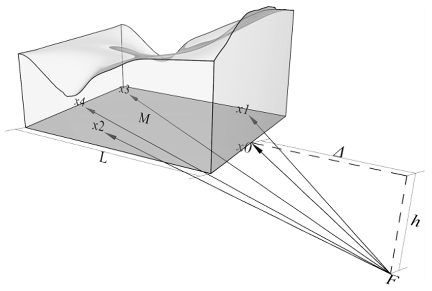
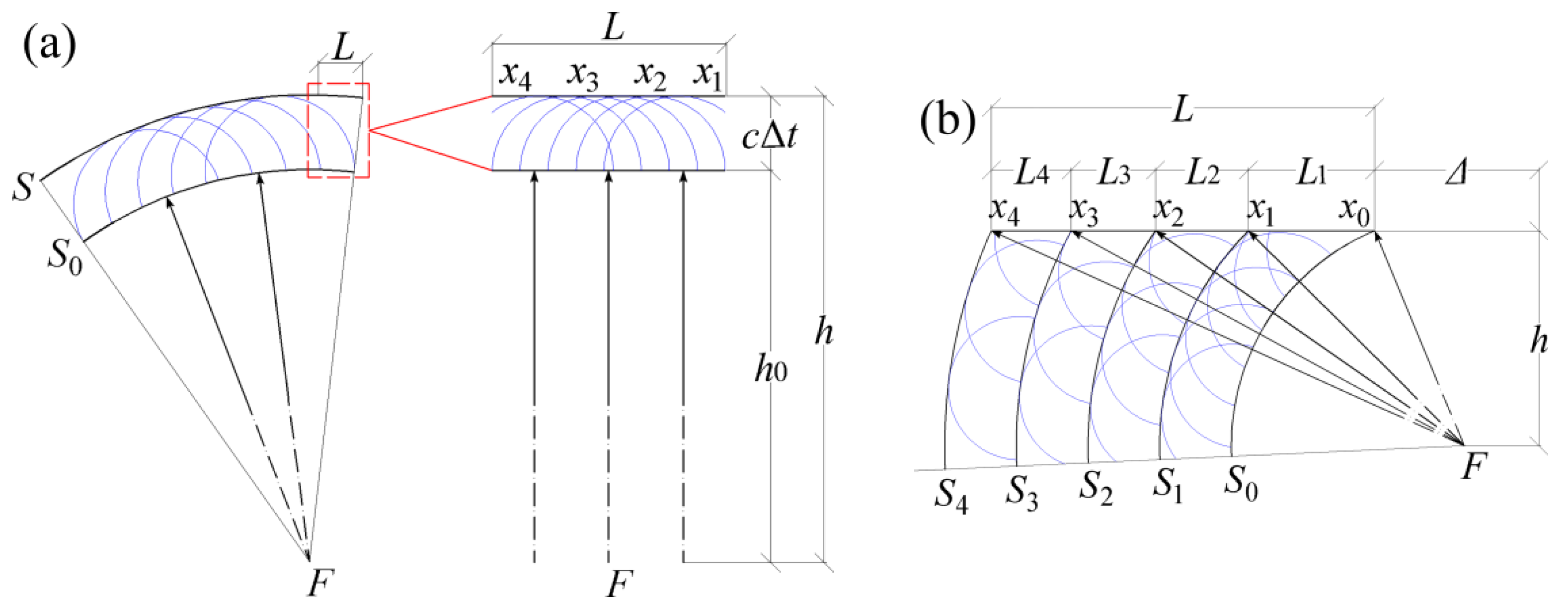
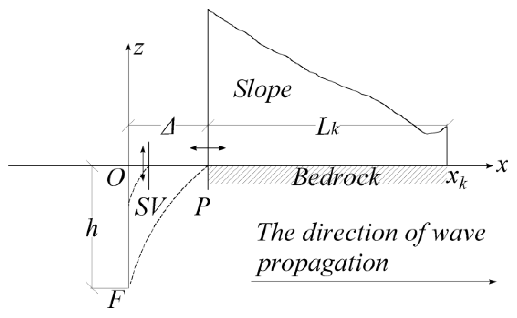
2. The Model for Non-Uniform Seismic Excitation Considering the Slope Scale

2.1. The Analytical Model of Non-Uniform Incidence Based on the Hilbert’s Best Approximation Problem (BAP)

As shown in Figure 1, a cluster of seismic waves is present from the hypocenter $F$ to the base of the slope. The length of the slope is $L$, the epicentral distance is $∆$, and the focal depth is $h$. Let the base be a set $M$ of several points $\left\{x=x_k\left|k=\mathrm{0,1},2\cdots \right.\right\}$. A Hilbert space $\mathbb{H}$ is constructed, and $M\subset \mathbb{H}$ is a complete convex subset. According to Hilbert’s best approximation principle (BAP), there exists the unique best approximation point $x_0\in M$ for $\forall F\in \mathbb{H}$ such that

$$‖F-x_0‖=d\left(F,M\right)=\underset{x\in M}{\inf }‖F-x‖$$

(1)

where $d\left(F,M\right)$ denotes the distance from the point $F$ to the set $M$, and inf denotes the infimum of a set. Meanwhile, $d\left(F,M\right)$ can be obtained as follows:

$$d\left(F,M\right)=\sqrt{{∆}^2+h^2}$$

(2)

As a complete convex subset of $\mathbb{H}$, $M$ has the following properties: $x_i$ and $x_j$ are any two points in $M$, and the set of the points $\left\{\mathsf{\alpha }{x}_i+\left(1-\mathsf{\alpha }\right)x_j\left|0\le \mathsf{\alpha }\le 1\right.\right\}\subset M$.

Therefore, the seismic waves arriving at the base from $F$ at the same moment are non-uniform. This is very different from the uniform incidence based on the plane-wave hypothesis. To further discriminate these two situations, the profiled two-dimensional models (Figure 2) are established to explain the generation of the seismic wave front under different assumptions based on Huygens principle.

Under the assumption shown in Figure 2a, the base of the slope $L$ can be considered as a tiny arc of the sphere if the hypocenter $F$ is far enough away. Obviously, the set of all points on $L$ does not satisfy the conditions of the convex set, and therefore the unique best approximation point $x_0$ does not exist. The spherical wave emitted from each point on the wave front $S_0$ at the moment $t$ forms a spherical surface with radius $R$ after $\mathsf{\Delta }t$ time. The envelope $S$ of these sub-waves becomes the new wave front at the moment of $t+\mathsf{\Delta }t$ in the forward direction of the wave. Each point on $L$ has the same phase and distance from $F$. In other words, the base of the slope is an isophase surface. Accordingly, the moveout equation of uniform incidence can be expressed as follows:

$$\left\{\begin{array}{l}{t}_0={\displaystyle \frac{h_0}{c}}\\ t_k={\displaystyle \frac{h}{c}}\left(k=\mathrm{1,2},3\dots \right)\end{array}\right.$$

(3)

where $t_0$ denotes the time required for the seismic wave to propagate to $S_0$, $t$ denotes the time required for the seismic wave to propagate to $S$, and $c$ denotes the apparent velocity of propagation of seismic waves.

Under the assumption of Figure 2b, the set of all points on $\mathrm{L}$ is a complete convex subset in $\mathbb{H}$ that satisfies Hilbert’s best approximation condition. The spherical wave emitted from each point on the wave front $S_0$ at the same moment $\mathrm{t}$ forms different envelopes of wave front. Seismic waves incident on $\mathrm{L}$ from $\mathrm{F}$ are non-uniform. Accordingly, the moveout equation of non-uniform incidence can be expressed as follows:

$$\left\{\begin{array}{l}{t}_0^{\prime }={\displaystyle \frac{\sqrt{{∆}^2+h^2}}{c}}\\ t_k^{\prime }={\displaystyle \frac{\sqrt{{\left(∆+L_k\right)}^2+h^2}}{c}}\left(k=\mathrm{1,2},3\dots \right)\end{array}\right.$$

(4)

where $t_0^{\prime }$ denotes the time required for the seismic wave to propagate to $S_0$, $t_k^{\prime }$ denotes the time required for the seismic wave to propagate to $S_k$, $∆$ denotes the epicentral distance, and $h$ denotes the focal depth.

Comparing the two forms of incidence, the relationship between $t_k$ and $t_k^{\prime }$ can be expressed as follows:

$${\displaystyle \frac{t_k}{t_k^{\prime }}}={\displaystyle \frac{h}{\sqrt{{\left(∆+L_k\right)}^2+h^2}}}={\displaystyle \frac{1}{\sqrt{{\left[\left(∆+L_k\right)/h\right]}^2+1}}}$$

(5)

It can be concluded that if the slope scale satisfies BAP, seismic wave incidence is non-uniform. The non-uniform incidence mechanisms is inscribed by $∆/h+L/h$. Indeed, $∆/h$ denotes the angle of incidence of seismic waves, and the law of its variation on the dynamic response of slopes has been extensively studied. In this paper, $L/h$ is regarded as the variable of the slope scale to study the non-uniform dynamic response considering non-uniform seismic incidence. Meanwhile, $L/h$ is the foundation for determining whether the slope model is consistent with BAP or the plane wave assumption of Huygens’ principle.

For the study of the seismic dynamic response of large slopes, the non-uniform incidence model based on BAP is superior to traditional methods in that it can consider the relationship between epicenter distance and slope scale, as well as the influence of different incidence angles on the response acceleration, velocity and displacement of the slope.

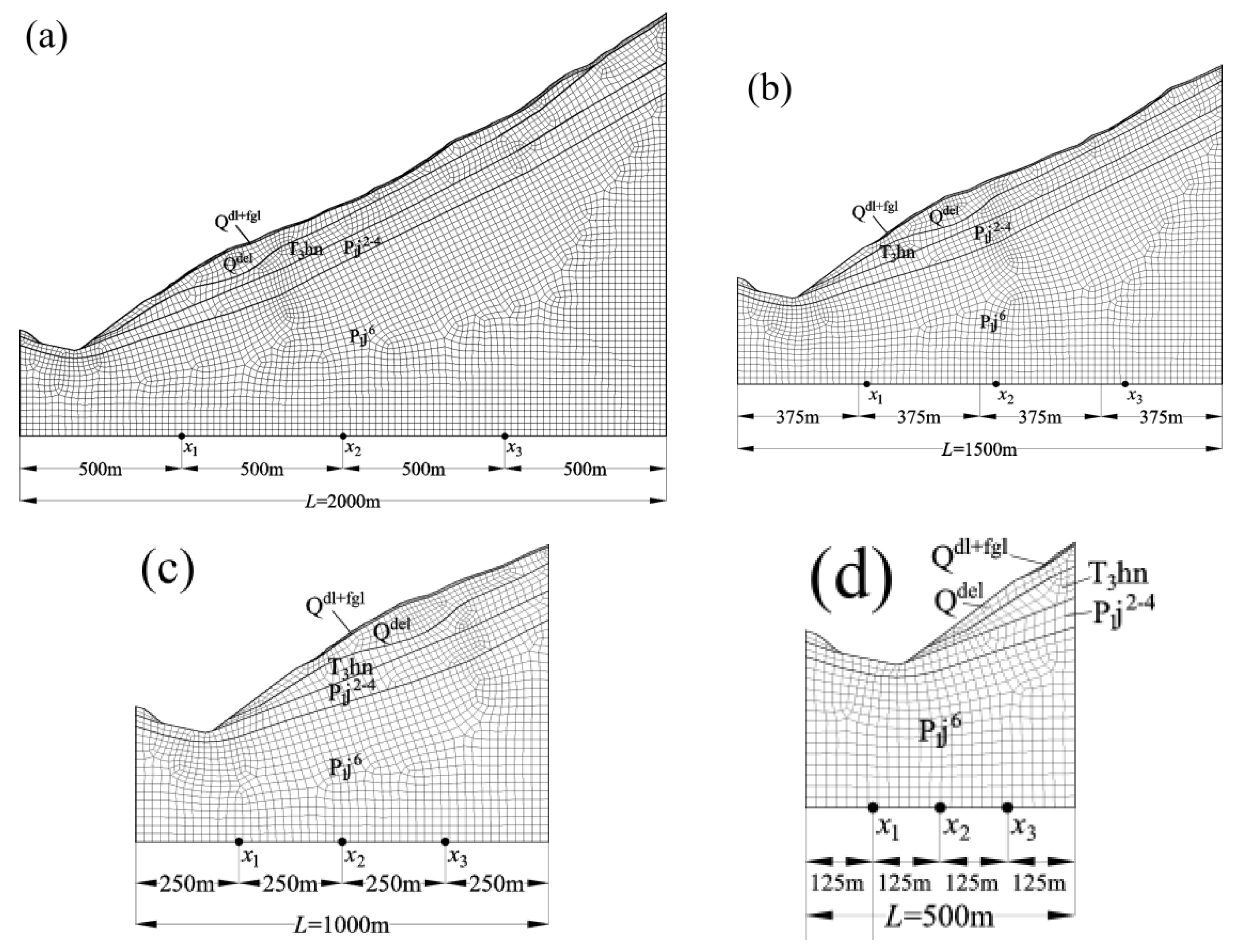
2.2. Numerical Models of Finite Difference Method (FDM) for Simulating Non-Uniform Incidence of Seismic Waves

In order to visually represent the non-uniform spatio-temporal dynamic response, numerical models of different scales based on the Finite Difference Method (FDM) are established. The diagrams of the slope simulation model are illustrated in Figure 3, and the material parameters of the slopes are listed in

Table 1. Material parameters of the slopes.

Stratigraphy	Density $\mathit{\rho }\left(\mathbf{g}/{\mathbf{c}\mathbf{m}}^3\right)$	Young’s Modulus $\mathit{E}\left(\mathbf{G}\mathbf{P}\mathbf{a}\right)$	Poisson’s Ratio $\mathit{\upsilon }$	Cohesion $\mathit{c}\left(\mathbf{M}\mathbf{P}\mathbf{a}\right)$	Friction $\mathit{\phi }\left(°\right)$
Qdl+fgl	2.30	0.1	0.35	0.016	18
Qdel	2.30	0.5	0.32	2.8	48.5
T3hn	2.35	5.0	0.25	0.1	22
P1j2−4	2.40	15.0	0.23	2.9	49
P1j6	2.45	20.0	0.20	3.5	48.5

. The Mohr–Coulomb model is adopted in this study. The maximum length of the model grid is 20 m and the minimum length is 10 m. The local non-viscous damping of 0.157 is adopted in the simulation.

An artificial seismic wave of type P-SV is generated based on GB 51247-2018 [24] to simulate the seismic waves (both uniform incidence and non-uniform incidence), and the peak ground acceleration (PGA) of the wave is $1.35\mathrm{m}/{\mathrm{s}}^2$. The input acceleration–time history and its Fourier spectrum are illustrated in Figure 4. In accordance with the methodology depicted in Figure 5, seismic waves are applied as velocity tables to the model in FDM in this paper.

The application of primary waves and shear waves to the grid points can be expressed as

$$\left\{\begin{array}{l}{v}_{ij}^k=\mathrm{Table}\left(v^k,∆t_p^k\right)·e_{ij}\left(t>t_p\right)\\ v_{ij}^{k+1}=v_{ij}^k+\mathrm{Table}\left(v^{k+1},∆t_s^{k+1}\right)·e_{ji}\left(t>t_s\right)\end{array}\right.$$

(6)

where $v^k$ denotes the velocity of the grid points for the $k$th computational step. $e_{ij}$ denotes the unit vector of coordinates. $\mathrm{T}\mathrm{a}\mathrm{b}\mathrm{l}\mathrm{e}\left(v^k,∆t_p^k\right)$ denotes the value of the velocity table of seismic waves. $t$ denotes the dynamic time step of the model. $t_p$ and $t_s$ denote the time of arrival of primary waves and shear waves at the grid points, respectively.

3. The Non-Uniform Spatio-Temporal Dynamic Response of the Seismic Interface

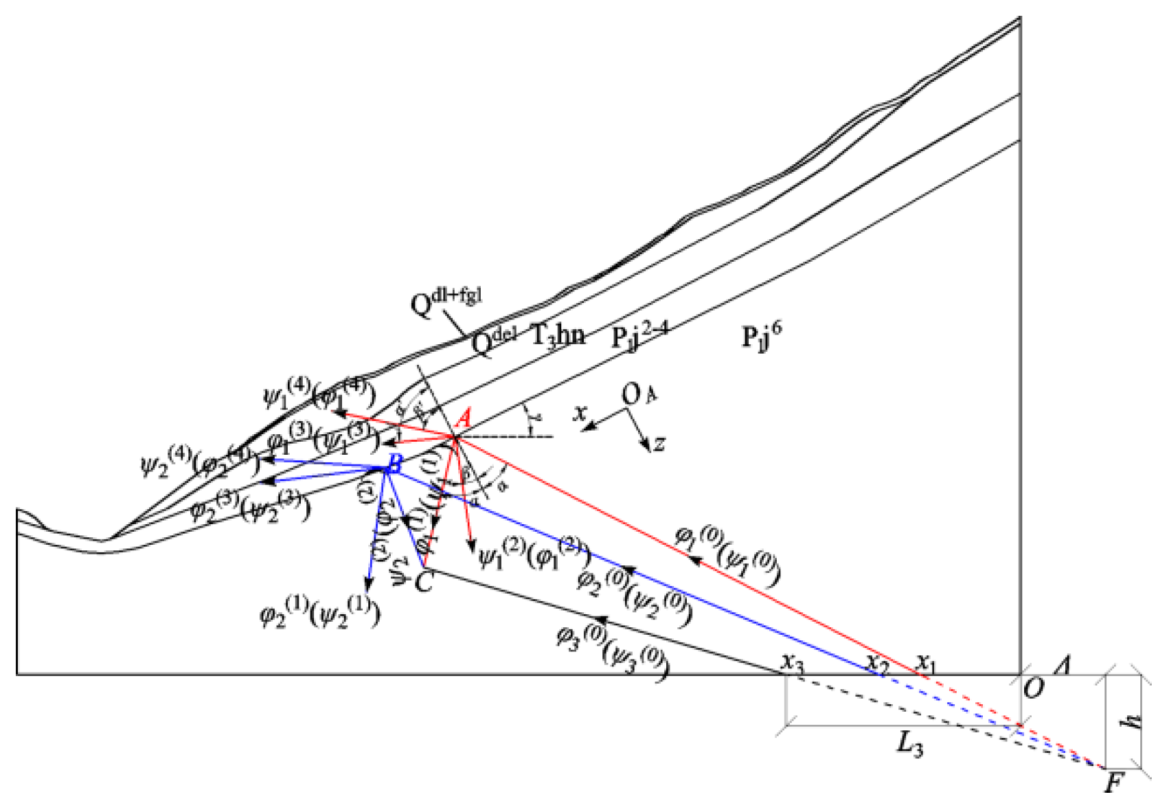
3.1. Stoneley Equation Considering the Scale of the Slope on the Interface

Simplified diagrams are designed to illustrate the model of non-uniform wave incidence. As shown in Figure 6, a non-uniform P-SV type of surface wave, designated the Stoneley wave, is observed on the interface at the base of the slope. The displacement potential function of the wave can be expressed as follows:

$$\left\{\begin{array}{l}{\phi }^{\left(1\right)}=A_1\exp \left[-{\alpha }_{1}z+i\left(k_{\mathrm{S}\mathrm{T}}x-\omega t\right)\right]\\ {\psi }^{\left(1\right)}=B_1\exp \left[-{\beta }_{1}z+i\left(k_{\mathrm{S}\mathrm{T}}x-\omega t\right)\right]\\ {\phi }^{\left(2\right)}=A_2\exp \left[{\alpha }_{2}z+i\left(k_{\mathrm{S}\mathrm{T}}x-\omega t\right)\right]\\ {\psi }^{\left(2\right)}=B_2\exp \left[{\beta }_{2}z+i\left(k_{\mathrm{S}\mathrm{T}}x-\omega t\right)\right]\end{array}\right.$$

(7)

where $\phi$ and $\psi$ denote the displacement potential functions of P and SV waves, respectively. The superscript “(1)” indicates a medium with a positive z-value, and the superscript “(2)” indicates a medium with a negative z-value. $A_1$, $B_1$, $A_2$, and $B_2$ denote the amplitude of each function. $k_{\mathrm{S}\mathrm{T}}$ denotes the number of the wave, $\omega$ denotes the circular frequency of the wave. $\alpha$ and $\beta$ can be expressed as follows:

$$\left\{\begin{array}{l}{\alpha }_j^2=k_{\mathrm{S}\mathrm{T}}^2-{\omega }^2/c_{Pj}^{2}j=\mathrm{1,2}\\ {\beta }_j^2=k_{\mathrm{S}\mathrm{T}}^2-{\omega }^2/c_{Sj}^{2}j=\mathrm{1,2}\begin{array}{c}\\ \end{array}\end{array}\right.$$

(8)

where $c_P$ denotes the velocity of the pressure wave, and $c_S$ denotes the velocity of the shear wave.

The displacement can be expressed by the displacement potential function as follows:

$$\left\{\begin{array}{l}{u}_x={\displaystyle \frac{\mathsf{\partial }\phi }{\mathsf{\partial }x}}-{\displaystyle \frac{\mathsf{\partial }\psi }{\mathsf{\partial }z}}\\ u_z={\displaystyle \frac{\mathsf{\partial }\phi }{\mathsf{\partial }z}}+{\displaystyle \frac{\mathsf{\partial }\psi }{\mathsf{\partial }x}}\begin{array}{c}\\ \end{array}\end{array}\right.$$

(9)

where $u_x$ denotes the displacement on the x-axis, and $u_z$ denotes the displacement on the z-axis.

The dynamic mechanisms, defined as the stress component, can be expressed by the displacement potential function as

$$\left\{\begin{array}{l}{\sigma }_{zx}=\mu \left(2{\displaystyle \frac{{\mathsf{\partial }}^2\phi }{\mathsf{\partial }x\mathsf{\partial }z}}-{\displaystyle \frac{{\mathsf{\partial }}^2\psi }{\mathsf{\partial }{z}^2}}+{\displaystyle \frac{{\mathsf{\partial }}^2\psi }{\mathsf{\partial }{x}^2}}\right)\\ {\sigma }_{zz}=\lambda \left({\displaystyle \frac{{\mathsf{\partial }}^2\phi }{\mathsf{\partial }{x}^2}}+{\displaystyle \frac{{\mathsf{\partial }}^2\phi }{\mathsf{\partial }{z}^2}}\right)+2\mu \left({\displaystyle \frac{{\mathsf{\partial }}^2\phi }{\mathsf{\partial }{z}^2}}+{\displaystyle \frac{{\mathsf{\partial }}^2\psi }{\mathsf{\partial }x\mathsf{\partial }z}}\right)\begin{array}{c}\\ \end{array}\end{array}\right.$$

(10)

where $\lambda$ and $\mu$ denote the Lamé coefficient of the medium, and are related to the Young’s modulus $E$ and the Poisson’s ratio $\upsilon$.

At the interface, where $z=0$ at the base of the slope, the following boundary conditions are present:

$$\left\{\begin{array}{c}{\left.u_x^{\left(1\right)}\right|}_{z=0}={\left.u_x^{\left(2\right)}\right|}_{z=0}\\ {\left.u_z^{\left(1\right)}\right|}_{z=0}={\left.u_z^{\left(2\right)}\right|}_{z=0}\begin{array}{c}\\ \end{array}\end{array}\right.$$

(11)

$$\left\{\begin{array}{c}{\left.{\sigma }_{zx}^{\left(1\right)}\right|}_{z=0}={\left.{\sigma }_{zx}^{\left(2\right)}\right|}_{z=0}\\ {\left.{\sigma }_{zz}^{\left(1\right)}\right|}_{z=0}={\left.{\sigma }_{zz}^{\left(2\right)}\right|}_{z=0}\begin{array}{c}\\ \end{array}\end{array}\right.$$

(12)

Substituting Equation (8) into Equation (10), and substituting Equation (9) into Equation (11), the Stoneley equation can be obtained as

$$\left[\begin{array}{ccc}i{k}_{\mathrm{S}\mathrm{T}}& {\beta }_1& -i{k}_{\mathrm{S}\mathrm{T}}\\ -{\alpha }_1& i{k}_{\mathrm{S}\mathrm{T}}& -{\alpha }_2\\ \begin{array}{c}{\mu }_1\left(k_{\mathrm{S}\mathrm{T}}^2+{\beta }_1^2\right)\\ -2i{\mu }_1{\alpha }_1{k}_{\mathrm{S}\mathrm{T}}\end{array}& \begin{array}{c}-2i{\mu }_1{\beta }_1{k}_{\mathrm{S}\mathrm{T}}\\ -{\mu }_1\left(k_{\mathrm{S}\mathrm{T}}^2+{\beta }_1^2\right)\end{array}& \begin{array}{c}-{\mu }_2\left(k_{\mathrm{S}\mathrm{T}}^2+{\beta }_2^2\right)\\ -2i{\mu }_2{\alpha }_2{k}_{\mathrm{S}\mathrm{T}}\end{array}\end{array}\begin{array}{c}{\beta }_2\\ -i{k}_{\mathrm{S}\mathrm{T}}\\ \begin{array}{c}-2i{\mu }_2{\beta }_2{k}_{\mathrm{S}\mathrm{T}}\\ {\mu }_2\left(k_{\mathrm{S}\mathrm{T}}^2+{\beta }_2^2\right)\end{array}\end{array}\right]\left[\begin{array}{c}{A}_1\\ B_1\\ \begin{array}{c}{A}_2\\ B_2\end{array}\end{array}\right]=0$$

(13)

where $A$ and $B$ denote the amplitude of the displacement potential function of the seismic wave, and their values cannot be simultaneously 0.

Therefore, the homogeneous function (13) has a non-zero solution and the value of the determinant of its coefficient matrix is 0. Subsequently, the value of $k_{\mathrm{S}\mathrm{T}}$ can be obtained, and Equation (13) can be solved and substituted into Equation (7) to obtain the expression for the displacement component,

$$\begin{array}{l}{u}_x=u_x^{\left(1\right)}+u_x^{\left(2\right)}\\ =\left({\displaystyle \frac{{\mathsf{\partial }\phi }_1}{\mathsf{\partial }x}}+{\displaystyle \frac{{\mathsf{\partial }\phi }_2}{\mathsf{\partial }x}}\right)-\left({\displaystyle \frac{\mathsf{\partial }{\psi }_1}{\mathsf{\partial }z}}+{\displaystyle \frac{\mathsf{\partial }{\psi }_2}{\mathsf{\partial }z}}\right)\\ =i{k}_{\mathrm{S}\mathrm{T}}\left({\phi }_1+{\phi }_2\right)+{\beta }_1{\psi }_1-{\beta }_2{\psi }_2\end{array}$$

(14)

$$\begin{array}{l}{u}_z=u_z^{\left(1\right)}+u_z^{\left(2\right)}\\ =\left({\displaystyle \frac{{\mathsf{\partial }\phi }_1}{\mathsf{\partial }z}}+{\displaystyle \frac{{\mathsf{\partial }\phi }_2}{\mathsf{\partial }z}}\right)-\left({\displaystyle \frac{\mathsf{\partial }{\psi }_1}{\mathsf{\partial }x}}+{\displaystyle \frac{\mathsf{\partial }{\psi }_2}{\mathsf{\partial }x}}\right)\\ =-{\alpha }_1{\phi }_1+{\alpha }_2{\phi }_2+i{k}_{\mathrm{S}\mathrm{T}}\left({\psi }_1+{\psi }_2\right)\end{array}$$

(15)

By substituting Equation (4) into Equations (13) and (14), the expression for the displacement component considering the scale of the slope on the interface is obtained:

$$\begin{gathered} \mathrm{R}\mathrm{e}\left({\left.u_x\right|}_{z=0}\right)=-k_{\mathrm{S}\mathrm{T}}\left(A_1+A_2\right)\sin \left[k_{\mathrm{S}\mathrm{T}}{x}_k-\omega h\sqrt{{1+\left[\left(∆/h\right)+\left(L_k/h\right)\right]}^2}/c\right] \\ +\left(B_1{\beta }_1-B_2{\beta }_2\right)\cos \left[k_{\mathrm{S}\mathrm{T}}{x}_k-\omega h\sqrt{{1+\left[\left(∆/h\right)+\left(L_k/h\right)\right]}^2}/c\right] \end{gathered}$$

(16)

$$\begin{array}{l}\mathrm{R}\mathrm{e}\left({\left.u_z\right|}_{z=0}\right)=-k_{\mathrm{S}\mathrm{T}}\left(B_1+B_2\right)\sin \left[k_{\mathrm{S}\mathrm{T}}{x}_k-\omega h\sqrt{{1+\left[\left(∆/h\right)+\left(L_k/h\right)\right]}^2}/c\right]\\ +\left(-A_1{\alpha }_1+A_2{\alpha }_2\right)\cos \left[k_{\mathrm{S}\mathrm{T}}{x}_k-\omega h\sqrt{{1+\left[\left(∆/h\right)+\left(L_k/h\right)\right]}^2}/c\right]\end{array}$$

(17)

According to the Fourier transform, the displacement potential function of the actual seismic waves can be decomposed into integrals of plane waves of different $\omega$, and Equation (7) can be written as

$$\left\{\begin{array}{l}\phi ={\int }_0^{\infty }A\left(\omega \right)\mathrm{e}\mathrm{x}\mathrm{p}\left[\mp \alpha z+i\left(k_{\mathrm{S}\mathrm{T}}x-\omega t\right)\right]\mathrm{d}\omega \\ \psi ={\int }_0^{\infty }B\left(\omega \right)\mathrm{e}\mathrm{x}\mathrm{p}\left[\mp \beta z+i\left(k_{\mathrm{S}\mathrm{T}}x-\omega t\right)\right]\mathrm{d}\omega \end{array}\right.$$

(18)

The displacement expressions similar to Equations (16) and (17) can be obtained by substituting the solution of Equation (13) into Equation (18).

It can be concluded that the value of the displacement on the interface at the base of the slope varies with $L_k$ at the same moment $t$, and the variation patterns are subjected to $L/h$. Such a non-uniform spatio-temporal dynamic response is caused by non-uniform seismic wave incidence, in which the slope scale plays an important role.

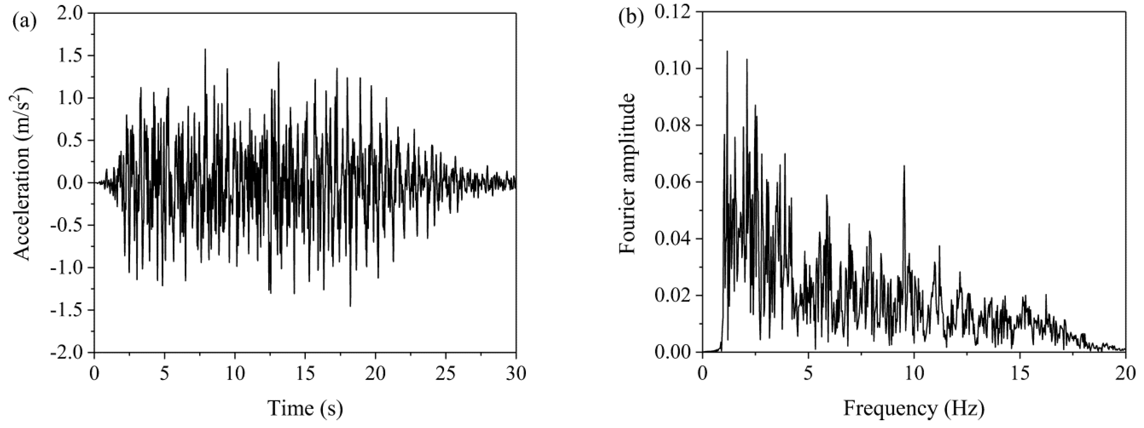
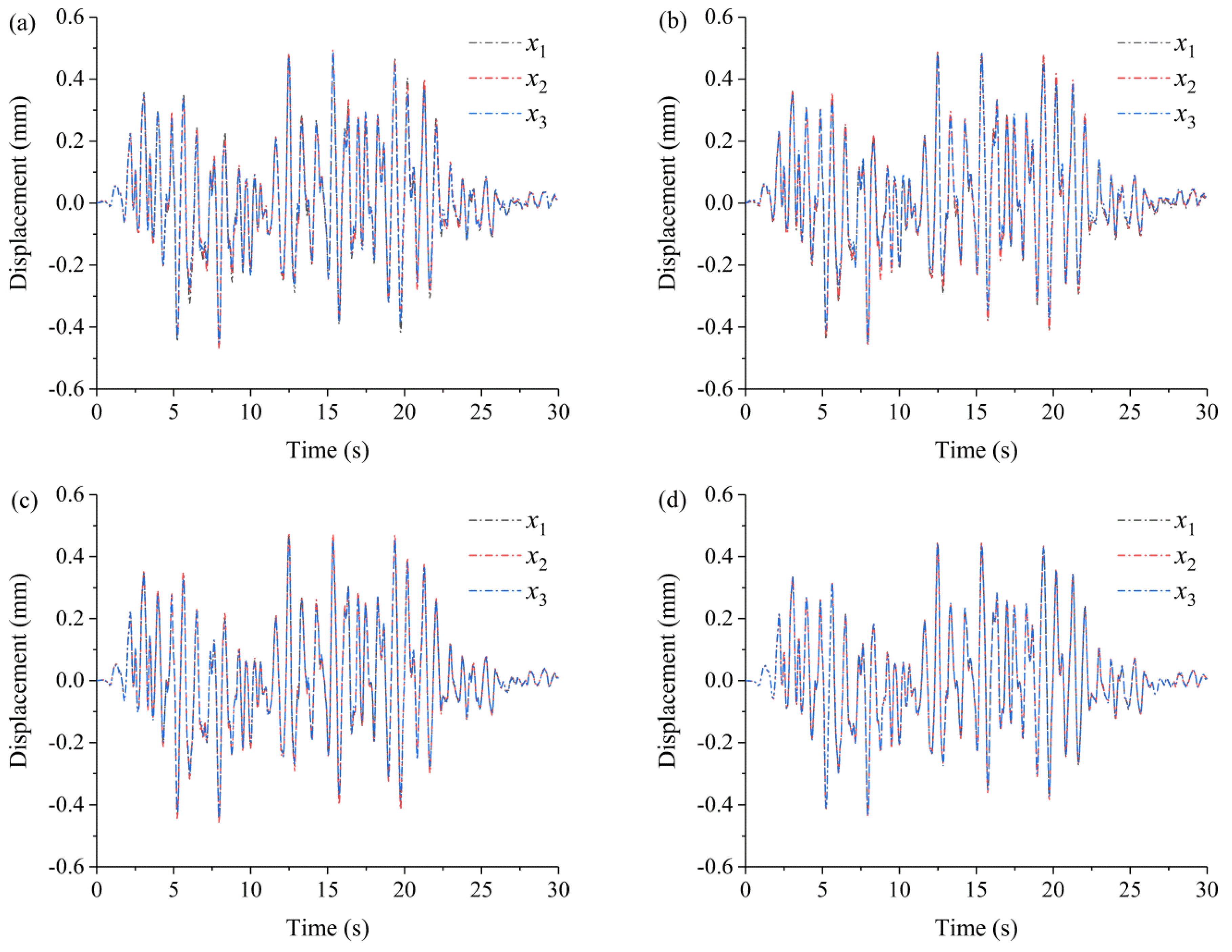
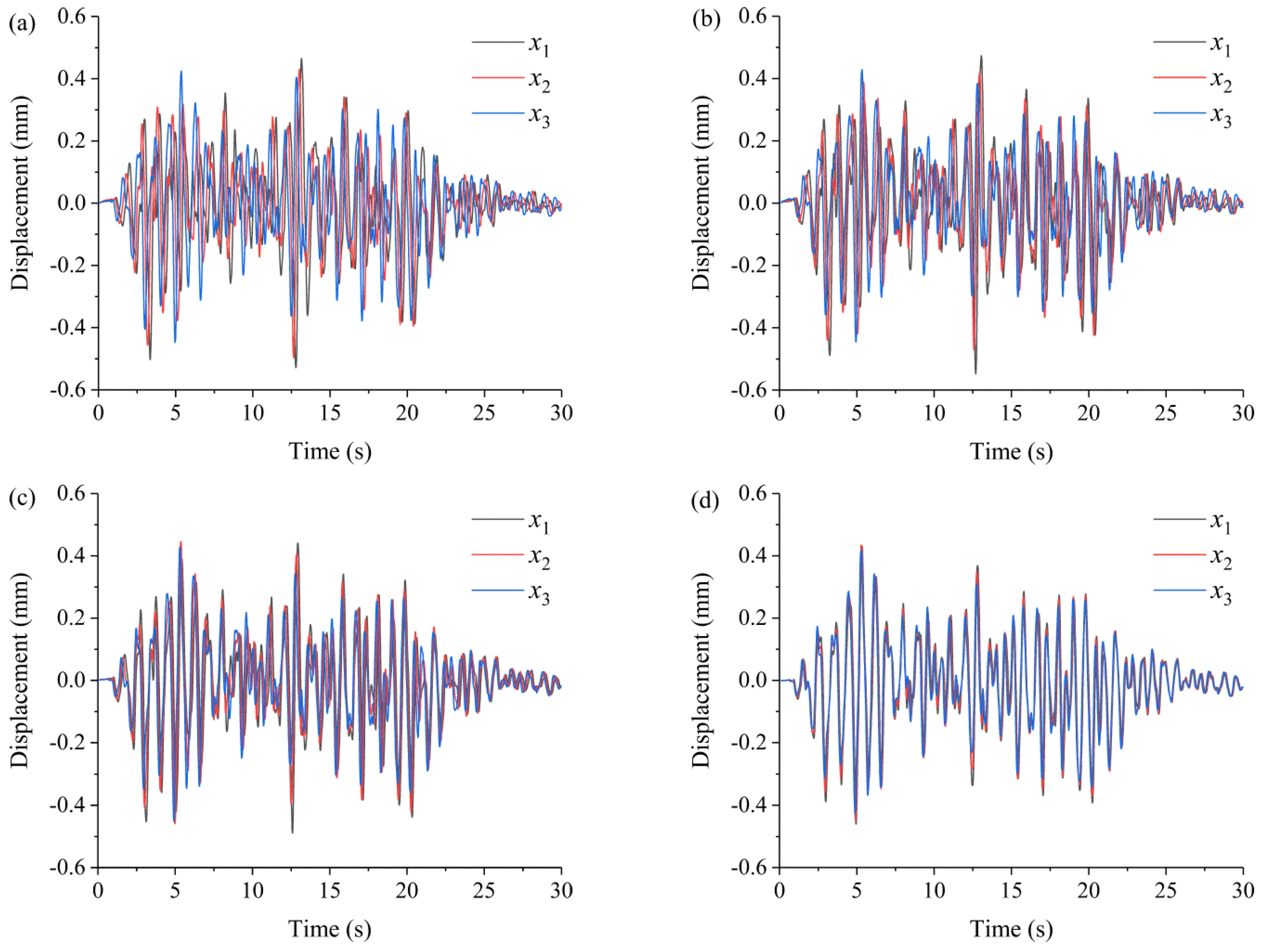
3.2. Numerical Simulation for the Non-Uniform Spatio-Temporal Dynamic Response of the Slope

Different scale models are established to simulate the spatio-temporal dynamic response. As mentioned in Section 2.2, the dynamic mechanisms of the slope model (Equation (10)) can be handled by the dynamic configuration of FDM. Besides this, quiet boundaries (viscous boundaries) are applied to both at the base and at the side boundaries of the models to simulate the boundary conditions as in Equations (11) and (12). Moreover, observation points $x_1$, $x_2$ and $x_3$ on the interface at the base of the slope are set to record the variation of displacement in accordance with Equations (16) and (17).

Variations of $u_x$ with the time of slope observation points $\left(x_1,x_2,x_3\right)$ on the interface $\left(z=0\right)$ with different scales are illustrated in Figure 7 and Figure 8. The variations in displacement demonstrate that the inharmonic vibration of the observation points occurs in response to the seismic excitation. In the case of uniform incidence (Figure 7a–d), the displacements curves of each observation point vary in a synchronous manner. In the case of non-uniform incidence (Figure 8a–d), the displacements curves of each observation point exhibit different degrees of frequency and phase dispersion. Notably, as $L/h$ increases, there is a more marked dispersion in the frequency and phase of the displacements at each observation point. As $L/h$ decreases, the displacement curves at each observation point tend to be consistent.

Contours of $u_x$ in the slope models with different scales at the moment $t=15\mathrm{s}$ are presented in Figure 9 and Figure 10. In the case of uniform incidence (Figure 9), the values of the displacements are found to be in the same contour on the interface at the base of the slope. Conversely, in the case of non-uniform incidence (Figure 10a–d), different contours of the displacements are presented on the interface at the base of the slope. Notably, as $L/h$ increases, the contours of the displacements tend to be more discrete. As $L/h$ decreases, the contours of the displacements tend to be continuous.

In conclusion, the variations in the displacements on the interface at the base of the slope present a degree of spatio-temporal dispersibility in the dynamic response subjected to non-uniform seismic wave incidence. In the case of non-uniform incidence, the displacements exhibit different degrees of frequency and phase dispersion. The degree of dispersion increases with $L/h$; in other words, the non-uniformity of the dynamic response keeps the same tendency as $L/h$. In this paper, the numerical simulation results of the displacement contours indicate that the non-uniform spatio-temporal dynamic response cannot be disregarded in the case of $L/h>4:20$. Slopes of this scale subjected to seismic wave incidence satisfy the BAP principle. Conversely, the dynamic response exhibits uniformity in the case of $L/h<1:20$, which is in accordance with the plane wave assumption of Huygens’ principle.

4. The Dynamic Amplification Effect of Large-Scale Slope Subjected to the Non-Uniform Seismic Waves

4.1. Amplification Factor of Spectral Response Accelerations (SRA) Subjected to the Non-Uniform Seismic Waves

As illustrated in Figure 11, in the coordinate system $x{o}_{A}z$, the wave function of a P wave (or SV wave) incident from $x_j$ to a point (at the interface between P₁j⁶ and P₁J²⁻⁴) can be written as follows (in terms of P wave),

$$\left\{\begin{array}{c}{\phi }_j^{\left(0\right)}=A_j^{\left(0\right)}\exp \left[i\left(\omega t-k_x^{\left(0\right)}x-k_z^{\left(0\right)}z\right)\right]\\ {\phi }_j^{\left(1\right)}=A_j^{\left(1\right)}\exp \left[i\left(\omega t-k_x^{\left(1\right)}x+k_z^{\left(1\right)}z\right)\right]\\ {\psi }_j^{\left(2\right)}=A_j^{\left(2\right)}\exp \left[i\left(\omega t-k_x^{\left(2\right)}x+k_z^{\left(2\right)}z\right)\right]\\ {\phi }_j^{\left(3\right)}=A_j^{\left(3\right)}\exp \left[i\left(\omega t-k_x^{\left(3\right)}x-k_z^{\left(3\right)}z\right)\right]\\ {\psi }_j^{\left(4\right)}=A_j^{\left(4\right)}\exp \left[i\left(\omega t-k_x^{\left(4\right)}x-k_z^{\left(4\right)}z\right)\right]\end{array}\right.$$

(19)

where $\phi$ and $\psi$ denote the displacement potential functions of P and SV waves, respectively. The subscript “j” denotes that the seismic wave originates from point $x_j$ on the base. $k_x$ and $k_z$ denote the number of waves in the $x$ and $z$ directions, respectively, and can be defined as

$$\left\{\begin{array}{c}{k}_x^{\left(0\right)}=\omega /c_P^{\left(0\right)}·\sin \left(\alpha \right)\\ k_x^{\left(1\right)}=\omega /c_P^{\left(1\right)}·\sin \left(\alpha \right)\\ k_x^{\left(2\right)}=\omega /c_S^{\left(2\right)}·\sin \left(\beta \right)\\ k_x^{\left(3\right)}=\omega /c_P^{\left(3\right)}·\sin \left({\alpha }^{\prime }\right)\\ k_x^{\left(4\right)}=\omega /c_S^{\left(4\right)}·\sin \left({\beta }^{\prime }\right)\end{array}\right.$$

(20)

$$\left\{\begin{array}{c}{k}_z^{\left(0\right)}=\omega /c_P^{\left(0\right)}·\cos \left(\alpha \right)\\ k_z^{\left(1\right)}=\omega /c_P^{\left(1\right)}·\cos \left(\alpha \right)\\ k_z^{\left(2\right)}=\omega /c_S^{\left(2\right)}·\cos \left(\beta \right)\\ k_z^{\left(3\right)}=\omega /c_P^{\left(3\right)}·\cos \left({\alpha }^{\prime }\right)\\ k_z^{\left(4\right)}=\omega /c_S^{\left(4\right)}·\cos \left({\beta }^{\prime }\right)\end{array}\right.$$

(21)

where $c_P$ and $c_S$ denote the velocity of P and SV waves, respectively. $\omega$ denotes the circular frequency of the wave. $\alpha$, $\beta$, ${\alpha }^{\prime }$ and ${\beta }^{\prime }$ denote the incidence angle of the wave. $\gamma$ denotes the dip of the stratigraphy interface.

Substituting Equation (9) and Equation (10) into Equation (11) and Equation (12), respectively, the Knott equation can be obtained as

$$\left[\begin{array}{ccc}\sin \alpha & {\displaystyle \frac{c_P^{\left(0\right)}}{c_S^{\left(2\right)}·\cos \beta }}& -{\displaystyle \frac{c_P^{\left(0\right)}}{c_P^{\left(3\right)}·\sin {\alpha }^{\prime }}}\\ \cos \alpha & -{\displaystyle \frac{c_P^{\left(0\right)}}{c_S^{\left(2\right)}·\sin \beta }}& {\displaystyle \frac{c_P^{\left(0\right)}}{c_P^{\left(3\right)}·\cos {\alpha }^{\prime }}}\\ \begin{array}{c}\sin 2\alpha \\ \cos 2\beta \end{array}& \begin{array}{c}{\left[{\displaystyle \frac{c_P^{\left(0\right)}}{c_S^{\left(2\right)}}}\right]}^2\cos 2\beta \\ -\sin 2\beta \end{array}& \begin{array}{c}{\left[{\displaystyle \frac{c_P^{\left(0\right)}}{c_P^{\left(3\right)}}}\right]}^2{\left[{\displaystyle \frac{c_S^{\left(4\right)}}{c_S^{\left(2\right)}}}\right]}^2{k}_{\rho }\sin 2{\alpha }^{\prime }\\ -k_{\rho }\cos 2{\beta }^{\prime }\end{array}\end{array}\begin{array}{c}{\displaystyle \frac{c_P^{\left(0\right)}}{c_S^{\left(4\right)}}}·\cos {\beta }^{\prime }\\ {\displaystyle \frac{c_P^{\left(0\right)}}{c_S^{\left(4\right)}}}·\sin {\beta }^{\prime }\\ \begin{array}{c}-k_{\rho }{\left[{\displaystyle \frac{c_P^{\left(0\right)}}{c_S^{\left(2\right)}}}\right]}^2\cos 2{\beta }^{\prime }\\ -k_{\rho }\sin 2{\beta }^{\prime }\end{array}\end{array}\right]\left[\begin{array}{c}{R}_{10}\\ R_{20}\\ \begin{array}{c}{R}_{30}\\ R_{40}\end{array}\end{array}\right]=\left[\begin{array}{c}-\sin \alpha \\ \cos \alpha \\ \begin{array}{c}\sin 2\alpha \\ -\cos 2\beta \end{array}\end{array}\right]$$

(22)

where $k_{\rho }={\rho }_2/{\rho }_1$ denotes the ratio of rock densities in different stratigraphies. $R_{j0}=A_j/A_0$ denotes the amplitude ratio of the waves.

Under the superposition of multiple waves, the displacement potential function of point C can be expressed as

$$\left\{\begin{array}{l}{\phi }^{\left(C\right)}={\phi }_1^{\left(1\right)}+{\phi }_2^{\left(2\right)}+{\phi }_3^{\left(0\right)}\\ {\psi }^{\left(C\right)}={\psi }_1^{\left(1\right)}+{\psi }_2^{\left(2\right)}+{\psi }_3^{\left(0\right)}\end{array}\right.$$

(23)

Considering the non-uniform seismic wave incidence on the interface at the base of the slope, ${\phi }_3^{\left(0\right)}$ and ${\psi }_3^{\left(0\right)}$ can be expressed according to Equation (4),

$$\left\{\begin{array}{l}{\phi }_3^{\left(0\right)}={\phi }^{\left(0\right)}\left(\sqrt{{\left(∆+L_3\right)}^2+h^2}/c_P\right)\\ {\psi }_3^{\left(0\right)}={\psi }^{\left(0\right)}\left(\sqrt{{\left(∆+L_3\right)}^2+h^2}/c_S\right)\end{array}\right.$$

(24)

where ${\phi }^{\left(0\right)}$ and ${\phi }^{\left(0\right)}$ can be written as ${\phi }^{\left(1\right)}$ and ${\psi }^{\left(1\right)}$ in Equation (7), respectively. $L_3$ denotes the distance between $O$ and $x_3$. $∆$ denotes the epicentral distance. $h$ denotes the depth between hypocenter $F$ and the base of the slope.

${\phi }^{\left(C\right)}$ and ${\psi }^{\left(C\right)}$ can be solved by Equation (22) and substituted into Equation (9) to obtain $u^{\left(C\right)}$. Subsequently, the spectral response accelerations can be defined as

$$a_{\mathrm{m}\mathrm{a}\mathrm{x}}^{\left(C\right)}=\mathrm{m}\mathrm{a}\mathrm{x}\left|a_1^{\left(1\right)}+a_2^{\left(2\right)}+a_3^{\left(0\right)}\right|$$

(25)

Therefore, the acceleration amplification effect within the slope due to the superposition of waves scattering is caused by the non-uniform seismic wave incidence on the interface at the base. The acceleration amplification factor can be expressed as

$${\eta }^{\left(C\right)}={\displaystyle \frac{\mathrm{m}\mathrm{a}\mathrm{x}\left|a_1^{\left(1\right)}+a_2^{\left(2\right)}+a_3^{\left(0\right)}\right|}{a_0}}$$

(26)

where $a_0$ denotes the PGA of the seismic waves.

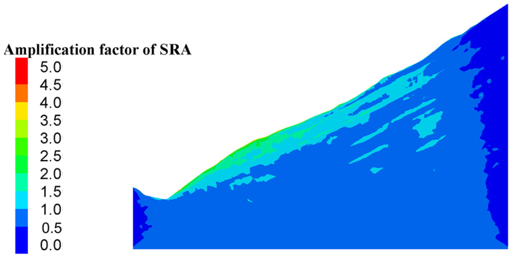
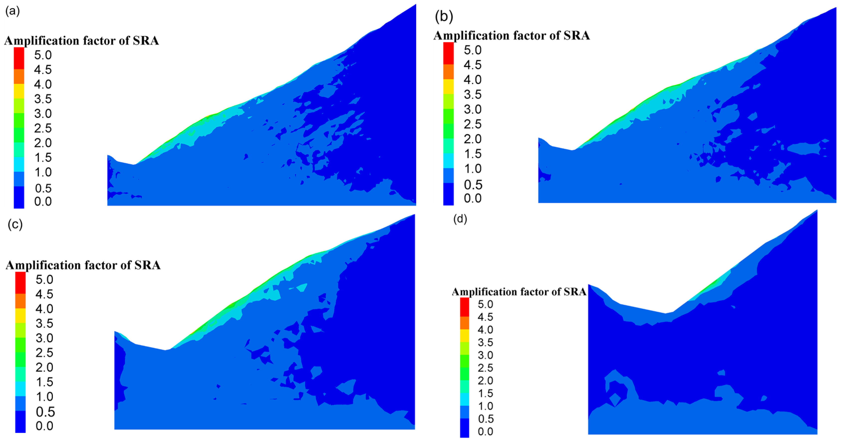
4.2. Numerical Simulation for Amplification Factor of SRA Considering the Scale of the Slope

Different scale models are established to simulate the acceleration amplification effect. Configurations of models in Section 2.2 are adopted, and the value of Equation (26) is represented by the contours of the amplification factor of SRA. As shown in Figure 12 and Figure 13, SRA are amplified from the base to the surface of the slope under the excitation of seismic waves. In the case of uniform incidence (Figure 12), the contours of amplification factor of SRA are found to have a layered distribution. Conversely, in the case of non-uniform incidence (Figure 13a–d), the amplification factor is concentrated on the slope surface. Notably, as $L/h$ increases, the magnification factor becomes increasingly concentrated, and the amplification effect becomes increasingly evident. It can be concluded that $L/h$ is a significant factor in the amplification effect of the non-uniform dynamic response.

In conclusion, the amplification effect at the surface of the slope presents a distribution of concentration in the dynamic response subjected to non-uniform seismic wave incidence. This result is consistent with those of Li et al. [20], who used the ABAQUS software platform to investigate the spatial variability characteristics of the seismic response at the ground surface under the influence of a traveling wave. With increases in bottom width, the amplification area caused by the terrain scattering effect gradually expands [25]. In the numerical simulation results of this paper, the non-uniformity of the dynamic amplification effect cannot be disregarded in the case of $L/h>4:20$. Slopes of this scale subjected to seismic wave incidence satisfy the BAP principle. Conversely, the dynamic response exhibits uniformity in the case of $L/h<1:20$, which is in accordance with the plane wave assumption of Huygens’ principle.

5. Discussion

In this paper, analytical models of the Stoneley and Knott equations are derived from the non-uniform incidence of P-SV waves in the $xoz$ coordinate plane. Meanwhile, both analytical models and numerical models are based on P-SV waves. Therefore, the non-uniform spatio-temporal dynamic response and the amplification factor of SRA are considered in this coordinate plane. The ratio of the slopes length and the focal depth $\left(L/h\right)$ is the foundation for determining whether the slope model is consistent with BAP or the plane-wave hypothesis, and the parameter that affects the degree of non-uniformity.

Indeed, the slopes are also influenced by SH waves, which cause polarization of the medium in the $xoy$ plane. The dynamic response of SH waves to slopes has also been studied based on a variety of methods. The analytical formulation in the framework of classical elastodynamics has been derived for the scattering of oblique incident plane SH waves by a semi-cylindrical canyon [26]. Based on a two-dimensional nonlinear seismic response analysis program, the impact of the incident angle of the SH wave on PGA and the response spectrum of ground motion has been studied [27]. Based on the indirect boundary integral equation method (IBIEM), trapezoidal valley surface ground motion characteristics and distribution laws under SH wave incidence have been analyzed [25,28]. Based on the indirect boundary element method, the response characteristics of different slopes under SH wave loading with various incident angles have been analyzed [29]. However, further study is required to gain a deeper understanding of the non-uniform spatio-temporal dynamic response and amplification effect caused by the slope scale. The coupling and superposition of SH and P-SV waves gives rise to a more complex dynamic response. Accordingly, the width of the slopes is also a significant variable in the following study.

Furthermore, large-scale slopes comprise a multitude of intricate stratigraphic sequences and geological formations, including fault lines and fissures. The scattering of seismic waves at discontinuous interfaces can also have an impact on the stability of slopes. For the jointed rock mass, the jointed material model can be employed to simulate its behavior as a continuum [30]. On the other hand, the discretization technique can be applied to study the failure mechanism for non-uniform soil slopes with varying soil strength parameters, which cannot be readily solved in conventional limit analysis [31,32]. The continuous–discontinuous method, combining the finite element method and discrete element method (FDEM), has been adopted to simulate the dynamic response and failure mechanism of the slope due to its entire process of seismic loads [33]. Although the FDM framework used in this study captures essential features of wave propagation and slope deformation, more granular approaches like the Dynamic Lattice Element Method (DLEM) could offer enhanced insight into localized failure mechanisms and cementation effects, particularly in heterogeneous rock slopes [34]. In future studies, the continuum–discontinuity numerical model can be used to explore the integration of multi-physics approaches—particularly those involving thermal–hydraulic–mechanical (THM) coupling to more accurately simulate the complex interactions within geomaterials under seismic loading. For instance, studies investigating cyclic thermal behavior in soils [35,36,37] highlight the significance of such interactions in transient response modeling.

6. Conclusions

In this paper, an analytical model based on the Hilbert’s best approximation problem (BAP) has been proposed to analyze the dynamic response of large-scale slopes under non-uniform seismic excitation. The analysis of the model of slopes has extended our knowledge of the non-uniform spatio-temporal dynamic response and amplification effect. Particularly, the seismic waves arriving at the large-scale slope base from the hypocenter at the same moment are non-uniform. This is very different from the uniform incidence based on the plane-wave hypothesis. The ratio of the slopes length and the focal depth $\left(L/h\right)$ is the foundation for determining whether the slope model is consistent with BAP or the plane-wave hypothesis, as well as the parameter that affects the degree of non-uniformity.

A non-uniform P-SV type of surface wave, designated the Stoneley wave, is designed to illustrate the model of non-uniform wave incidence. The value of the displacement on the interface at the base of the slope varies between different locations at the same moment, and the variation patterns are subjected to $L/h$. Such a non-uniform spatio-temporal dynamic response is caused by non-uniform seismic wave incidence. Meanwhile, the scattering model of elastic waves at rock interfaces is proposed to study the dynamic amplification effect of a large-scale slope subjected to non-uniform seismic waves. Considering the non-uniform seismic wave incidence on the interface at the base of the slope, the Knott equation is obtained. Eventually, the acceleration amplification factor is proposed.

Numerical models of the Finite Difference Method (FDM) and the artificial seismic wave have been applied to simulate the non-uniform incidence of seismic waves. The results of the numerical simulations provide an intuitive representation of the dynamic response of the slope under seismic incidence, as proposed by the analytical model. In the case of non-uniform incidence, the displacement curves of each observation point exhibit a range of frequencies and phases. The degree of dispersion is observed to increase with $L/h$, indicating that the non-uniformity of the dynamic response maintains a consistent tendency with $L/h$. The amplification effect at the surface of the slope exhibits a concentration of distribution in the dynamic response subjected to non-uniform seismic wave incidence. It is imperative to consider the non-uniform dynamic response when $L/h$ is greater than 4:20. Slopes of this scale, when subjected to seismic wave incidence, satisfy the BAP principle. Conversely, the dynamic response is observed to be uniform when $L/h$ is smaller than 1:20, which is in accordance with the plane wave assumption of Huygens’ principle. In this paper, only one geological model is studied, which has some limitations. In future studies, attention should be paid to large slopes with different geological conditions, such as open-pit mine slopes, highway trench slopes and reservoir bank slopes, to improve the results of the study.

References

1. Zhou, H.; Che, A.; Zhu, R. Damage Evolution of Rock Slopes Under Seismic Motions Using Shaking Table Test. Rock Mech. Rock Eng. 2022, 55, 4979–4997. [Google Scholar] [CrossRef]
2. Qi, X.; Zhang, Y. Stability analysis of soil-rock mixed slope under earthquake environment. Fresenius Environ. Bull. 2021, 30, 4384–4390. [Google Scholar]
3. Maleska, T.; Beben, D. Effect of the soil cover depth on the seismic response in a large-span thin-walled corrugated steel plate bridge. Soil Dyn. Earthq. Eng. 2023, 166, 107744. [Google Scholar] [CrossRef]
4. Schmit, C. Beginnings of a new science. D’Alembert’s Traite de dynamique and the French Royal Academy of Sciences around 1740. Centaurus 2017, 59, 285–299. [Google Scholar] [CrossRef]
5. Li, H.; Liu, Y.; Liu, L.; Liu, B.; Xia, X. Numerical evaluation of topographic effects on seismic response of single-faced rock slopes. Bull. Eng. Geol. Environ. 2019, 78, 1873–1891. [Google Scholar] [CrossRef]
6. Li, Y.; Wang, G.; Wang, Y. Parametric investigation on the effect of sloping topography on horizontal and vertical ground motions. Soil Dyn. Earthq. Eng. 2022, 159, 107346. [Google Scholar] [CrossRef]
7. Zhang, Z.; Fleurisson, J.; Pellet, F. The effects of slope topography on acceleration amplification and interaction between slope topography and seismic input motion. Soil Dyn. Earthq. Eng. 2018, 113, 420–431. [Google Scholar] [CrossRef]
8. Hill, D.P. Dynamic stresses, Coulomb failure, and remote triggering; corrected. Bull. Seismol. Soc. Amer. 2012, 102, 2313–2336. [Google Scholar] [CrossRef]
9. Shen, H.; Liu, Y.; Li, H.; Liu, B.; Xia, X.; Yu, C. Numerical evaluation of ground motion amplification of rock slopes under obliquely incident seismic waves. Soil Dyn. Earthq. Eng. 2024, 178, 108488. [Google Scholar] [CrossRef]
10. Shen, H.; Liu, Y.; Liu, B.; Li, H. Numerical study on the amplification effect of rock slopes under oblique incidence of seismic waves. Rock Soil Mech. 2023, 44, 2129–2142. [Google Scholar]
11. Shen, H.; Liu, Y.; Li, X.; Li, H.; Wang, L.; Huang, W. The combined amplification effects of topography and stratigraphy of layered rock slopes under vertically and obliquely incident seismic waves. Soil Dyn. Earthq. Eng. 2025, 193, 109331. [Google Scholar] [CrossRef]
12. Hao, M.; Zhang, Y. Analysis of Terrain Effect on the Properties of Ground Motion Due to Inclined SV Wave. Technol. Earthq. Disaster Prev. 2018, 13, 552–561. [Google Scholar]
13. Yin, C.; Li, W.; Zhao, C. Research of slope topographic amplification subjected to obliquely incident SV-waves. J. Vib. Eng. 2020, 33, 971–984. [Google Scholar]
14. Jiao, H.; Xie, J.; Zhao, M.; Huang, J.; Du, X.; Wang, J. Seismic response analysis of slope sites exposed to obliquely incident P waves. Front. Earth Sci. 2023, 10, 1057316. [Google Scholar] [CrossRef]
15. Wang, X.; Liu, C.; Yin, C.; Li, W. Stability Analysis of Soil Slopes with Oblique Incident Seismic Waves. J. Disaster Prev. Mitig. Eng. 2020, 40, 589–595. [Google Scholar]
16. Li, Z.; Li, J.; Liu, B.; Nie, M. Seismic motion amplification effect of shallow-cutting hill-canyon composite topography. J. Eng. Geol. 2021, 29, 137–150. [Google Scholar]
17. Huang, S.; Tao, R.; Wang, R. One simplified method for seismic stability analysis of an unsaturated slope considering seismic amplification effect. Geol. J. 2023, 58, 2388–2402. [Google Scholar] [CrossRef]
18. Zhou, J.; Zheng, Z.; Bao, T.; Tu, B.; Yu, J.; Qin, C. Assessment of rigorous solutions for pseudo-dynamic slope stability: Finite-element limit-analysis modelling. J. Cent. S. Univ. 2023, 30, 2374–2391. [Google Scholar] [CrossRef]
19. He, W.; Xiong, K.; Lu, X. Influence of deterministic spatial variation of motions on seismic response of gravity dam. J. Hydraul. Eng.-ASCE 2019, 50, 913–924. [Google Scholar]
20. Li, X.X.; Zhuang, H.Y.; Li, Z.Y.; Lu, L.T.; Zhao, K. Spatial seismic response of non-uniform wide river valley with multistage slopes in lower reaches of Yangtze River. Bull. Eng. Geol. Environ. 2023, 82, 279. [Google Scholar]
21. Lu, L.; Li, X.; Zhuang, H.; Wu, Q. Spatial variability characteristics of nonlinear seismic response in non-uniform engineering sites in the wide river valley. J. Earthq. Eng. Eng. Vib. 2023, 43, 216–225. [Google Scholar]
22. Xu, B.; Zhou, Y.; Zhou, C.; Kong, X.; Zou, D. Dynamic responses of concrete-faced rockfill dam due to different seismic motion input methods. Int. J. Distrib. Sens. Netw. 2018, 14, 15501477188. [Google Scholar] [CrossRef]
23. Isari, M.; Tarinejad, R.; Taghavighalesari, A.; Sohrabi-Bidar, A. A new approach to generating non-uniform support excitation at topographic sites. Soils Found. 2019, 59, 1933–1945. [Google Scholar] [CrossRef]
24. China MOWR. Standard for Seismic Design of Hydraulic Structurse. GB 51247-2018; The Ministry of Housing and Urban-Rural Development of the People’s Republic of China: Beijing, China, 2018. [Google Scholar]
25. Zhao, L.; Song, Z.; Wang, F.; Liu, Y.; Zhang, C. Non-uniform ground motion characteristics and influencing factors of valley site under oblique incidence of SH wave. J. Vib. Shock 2022, 41, 109–118, 128. [Google Scholar]
26. Zhang, N.; Gao, Y.; Pak, R.Y.S. Soil and topographic effects on ground motion of a surficially inhomogeneous semi-cylindrical canyon under oblique incident SH waves. Soil Dyn. Earthq. Eng. 2017, 95, 17–28. [Google Scholar] [CrossRef]
27. Zhu, C.; Zhang, J. Time-domain Nonlinear Seismic Response Analysis of Basin Surface due to Inclined SH Wave. Chin. J. Undergr. Space Eng. 2014, 10, 834–841. [Google Scholar]
28. Song, Z.; Zhao, L.; Wang, F.; Zhi, B.; Liu, Y. Ground motion characteristics analysis of sedimentary valley site with SH wave oblique incidence based on IBIEM. J. Vib. Shock 2023, 42, 1–10, 26. [Google Scholar]
29. Zhou, J.; Zhang, L. Dynamic Response Analysis of Slope Rock Mass with Complex Shape Based on Indirect Boundary Element Method. Earth Sci. 2022, 47, 4350–4361. [Google Scholar]
30. Huang, J.Q.; Zhao, M.; Xu, C.S.; Du, X.L.; Jin, L.; Zhao, X. Seismic stability of jointed rock slopes under obliquely incident earthquake waves. Earthq. Eng. Eng. Vib. 2018, 17, 527–539. [Google Scholar] [CrossRef]
31. Qin, C.; Chian, S.C.; Du, S. Revisiting seismic slope stability: Intermediate or below-the-toe failure? Geotechnique 2020, 70, 71–79. [Google Scholar] [CrossRef]
32. Chian, S.C.; Qin, C. Seismic Slope Stability with Discretization-Based Kinematic Analysis. In Proceedings of the Geotechnical Earthquake Engineering and Special Topics (Geo-Congress 2020), Minneapolis, MN, USA, 25–28 February 2020; pp. 284–294. [Google Scholar]
33. He, Y.; Cai, Z.; Wang, F.; Guo, C.; Xiang, B.; He, C.; Liu, E. Numerical investigation on slope stability influenced by seismic load and discontinuity with a continuous-discontinuous method. Bull. Eng. Geol. Environ. 2023, 82, 70. [Google Scholar] [CrossRef]
34. Rizvi, Z.H.; Mustafa, S.H.; Sattari, A.S.; Ahmad, S.; Furtner, P.; Wuttke, F. Dynamic Lattice Element Modelling of Cemented Geomaterials. In Advances in Computer Methods and Geomechanics, IACMAG 2019, Volume 1; Springer: Singapore, 2020; Volume 55, pp. 655–665. [Google Scholar]
35. Ahmad, S.; Rizvi, Z.H.; Arp, J.C.C.; Wuttke, F.; Tirth, V.; Islam, S. Evolution of Temperature Field around Underground Power Cable for Static and Cyclic Heating. Energies 2021, 14, 8191. [Google Scholar] [CrossRef]
36. Ahmad, S.; Rizvi, Z.; Khan, M.A.; Ahmad, J.; Wuttke, F. Experimental study of thermal performance of the backfill material around underground power cable under steady and cyclic thermal loading. Mater. Today-Proc. 2019, 17, 85–95. [Google Scholar] [CrossRef]
37. Ahmad, S.; Rizvi, Z.H.; Wuttke, F. Unveiling soil thermal behavior under ultra-high voltage power cable operations. Sci. Rep. 2025, 15, 7315. [Google Scholar] [CrossRef]
Figure 1. The model of non-uniform incidence of seismic waves. F denotes the hypocenter; denotes the epicentral distance; h denotes the focal depth; L denotes the length of the slope. x 0 , x 1 , x 2 , x 3 and x 4 denote different points at the base of the slope.
Applsci 15 05488 g001
Figure 2. Generation of the seismic wave front based on Huygens principle. (a) The form of uniform incidence; (b) the form of non-uniform incidence. S , S 0 , S 1 , S 2 , S 3 and S 4 denote wave fronts; F denotes the hypocenter; denotes the epicentral distance; h denotes the focal depth; L denotes the length of the slope; x 0 , x 1 , x 2 , x 3 and x 4 denote different points at the base of the slope.
Applsci 15 05488 g002
Figure 3. Diagrams of the slope simulation model with different scales: (a) L = 2000   m ,   L / h = 4 : 20 ; (b) L = 1500   m ,   L / h = 3 : 20 ; (c) L = 1000   m ,   L / h = 2 : 20 ; (d) L = 500   m ,   L / h = 1 : 20 ; h denotes the focal depth; L denotes the length of the slope. Qdl+fgl, Qdel, T3hn, P1j2−4 and P1j6 denote the designation of stratigraphy; x 1 , x 2 and x 3 are observation points.
Applsci 15 05488 g003
Figure 4. Artificial seismic wave with the PGA of 1.35   m / s 2 : (a) acceleration time history; (b) Fourier spectrum.
Applsci 15 05488 g004
Figure 5. Flowchart for the application of seismic waves.
Applsci 15 05488 g005
Figure 6. Diagram of non-uniform wave incidence. F denotes the hypocenter; denotes the epicentral distance; h denotes the focal depth; x k denotes any point at the base of the slope; L k denotes the length of the slope.
Applsci 15 05488 g006
Figure 7. Variations of u x with the time of slope observation points on the interface with different scales under uniform seismic incidence. (a) L = 2000   m ,     L / h = 4 : 20 ; (b) L = 1500   m ,   L / h = 3 : 20 ; (c) L = 1000   m ,   L / h = 2 : 20 ; (d) L = 500   m ,     L / h = 1 : 20 ; h denotes the focal depth; L denotes the length of the slope.
Applsci 15 05488 g007
Figure 8. Variations of u x with the time of slope observation points on the interface with different scales under non-uniform seismic incidence: (a) L = 2000   m ,   L / h = 4 : 20 ; (b) L = 1500   m ,   L / h = 3 : 20 ; (c) L = 1000   m ,   L / h = 2 : 20 ; (d) L = 500   m ,   L / h = 1 : 20 ; h denotes the focal depth; L denotes the length of the slope.
Applsci 15 05488 g008
Figure 9. Contours of u x of slope models with different scales at the moment t = 15   s under uniform seismic incidence (unit: m): L = 2000   m ,   L / h = 4 : 20 ; h denotes the focal depth; L denotes the length of the slope.
Applsci 15 05488 g009
Figure 10. Contours of u x of slope models with different scales at the moment t = 15   s under non-uniform seismic incidence (unit: m): (a) L = 2000   m ,   L / h = 4 : 20 ; (b) L = 1500   m ,   L / h = 3 : 20 ; (c) L = 1000   m ,   L / h = 2 : 20 ; (d) L = 500   m ,   L / h = 1 : 20 ; h denotes the focal depth; L denotes the length of the slope.
Applsci 15 05488 g010
Figure 11. The scattering of elastic waves at rock interfaces. F denotes the hypocenter; denotes the epicentral distance; h denotes the focal depth; Qdl+fgl, Qdel, T3hn, P1j2−4 and P1j6 denote the designation of stratigraphy; x 1 , x 2 and x 3 denote different points at the base of the slope. A and B denote different points on the interface; φ ψ denotes the displacement potential functions of P (or SV) waves. The seismic waves incident from points x 1 , x 2 , and x 3 are marked in red, blue, and black, respectively.
Applsci 15 05488 g011
Figure 12. Contours of amplification factor of SRA with different slope scales under uniform seismic incidence. L = 2000   m , L / h = 4 : 20 ; h denotes the focal depth; L denotes the length of the slope.
Applsci 15 05488 g012
Figure 13. Contours of amplification factor of SRA with different slope scales under non-uniform seismic incidence. (a) L = 2000   m ,   L / h = 4 : 20 ; (b) L = 1500   m ,   L / h = 3 : 20 ; (c) L = 1000   m ,   L / h = 2 : 20 ; (d) L = 500   m ,   L / h = 1 : 20 ; h denotes the focal depth; L denotes the length of the slope.
Applsci 15 05488 g013