
Monitoring and Analysis of Slope Geological Hazards Based on UAV Images


Abstract
1. Introduction
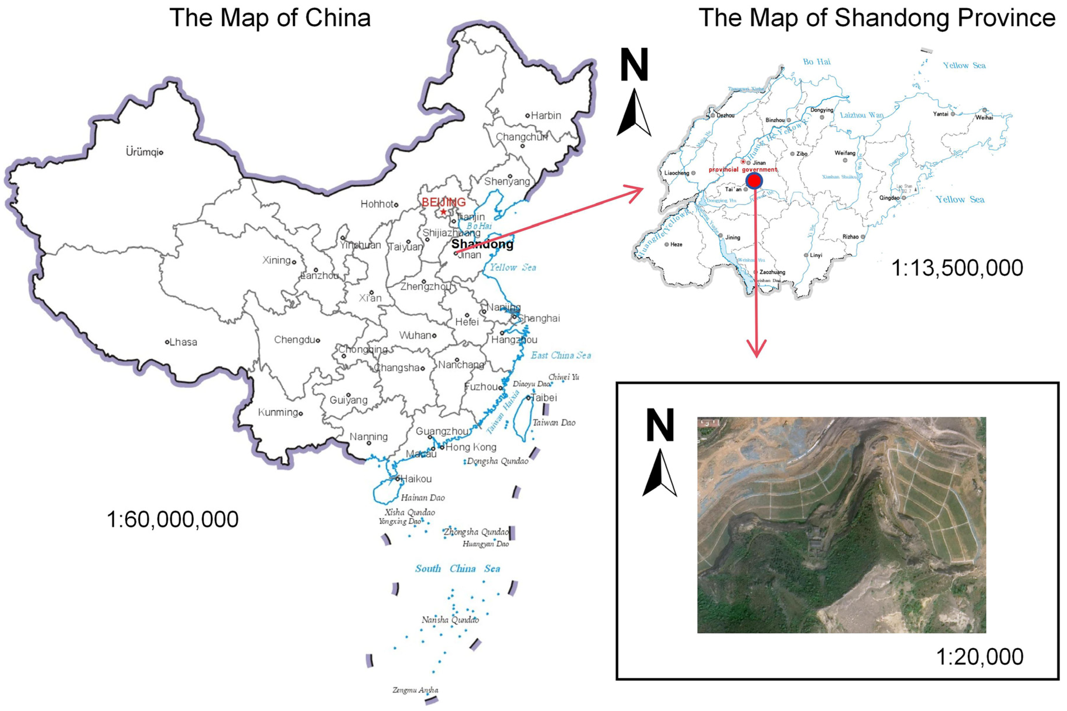
2. Study Area
3. Materials and Methods
3.1. UAV Survey System
3.2. UAV Remote Sensing Image Acquisition
3.3. Data Processing and Analysis
4. Remote Sensing Image Data Processing
4.1. Construct Models
4.1.1. Aerial Triangulation
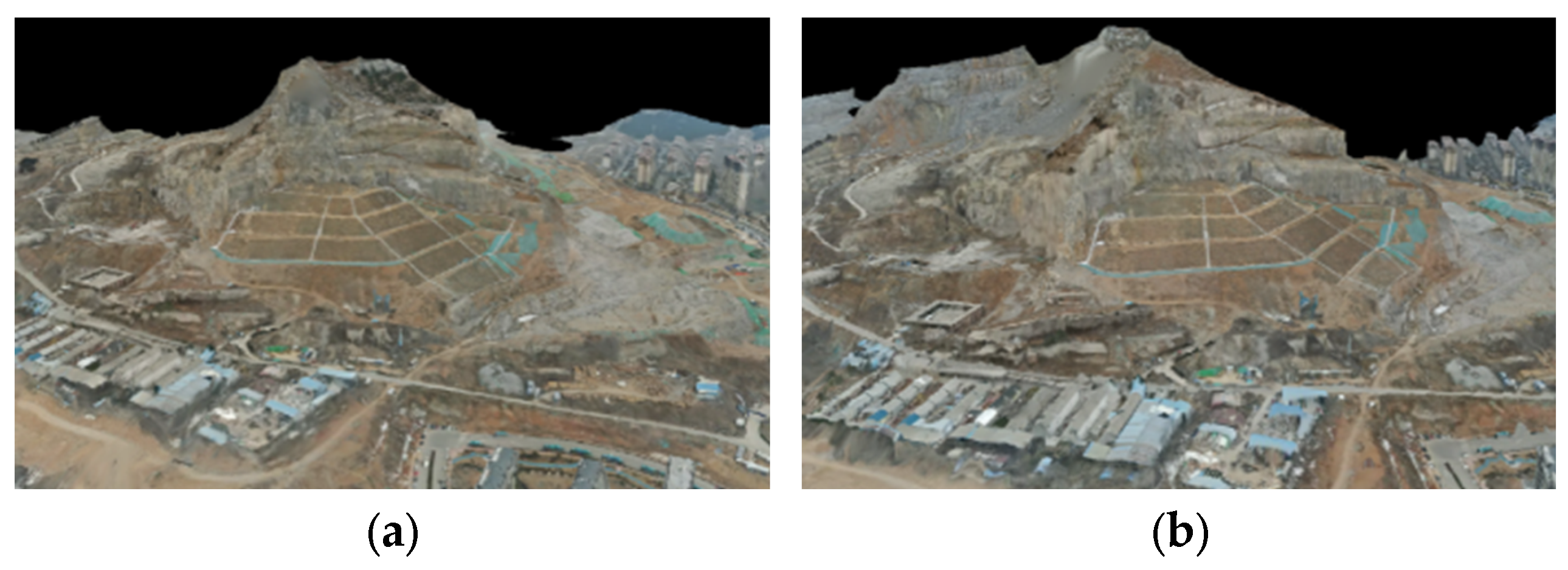
4.1.2. 3D Reconstruction
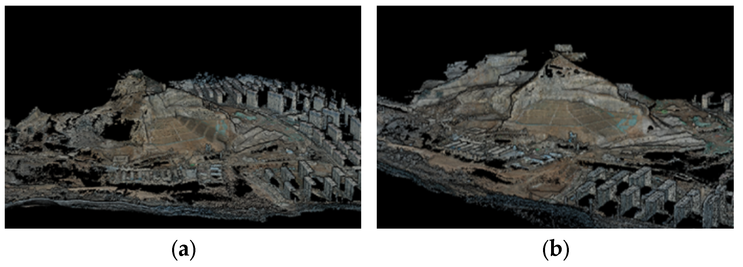
4.2. Point-Cloud Data Processing
4.2.1. Point-Cloud Data Pre-Processing
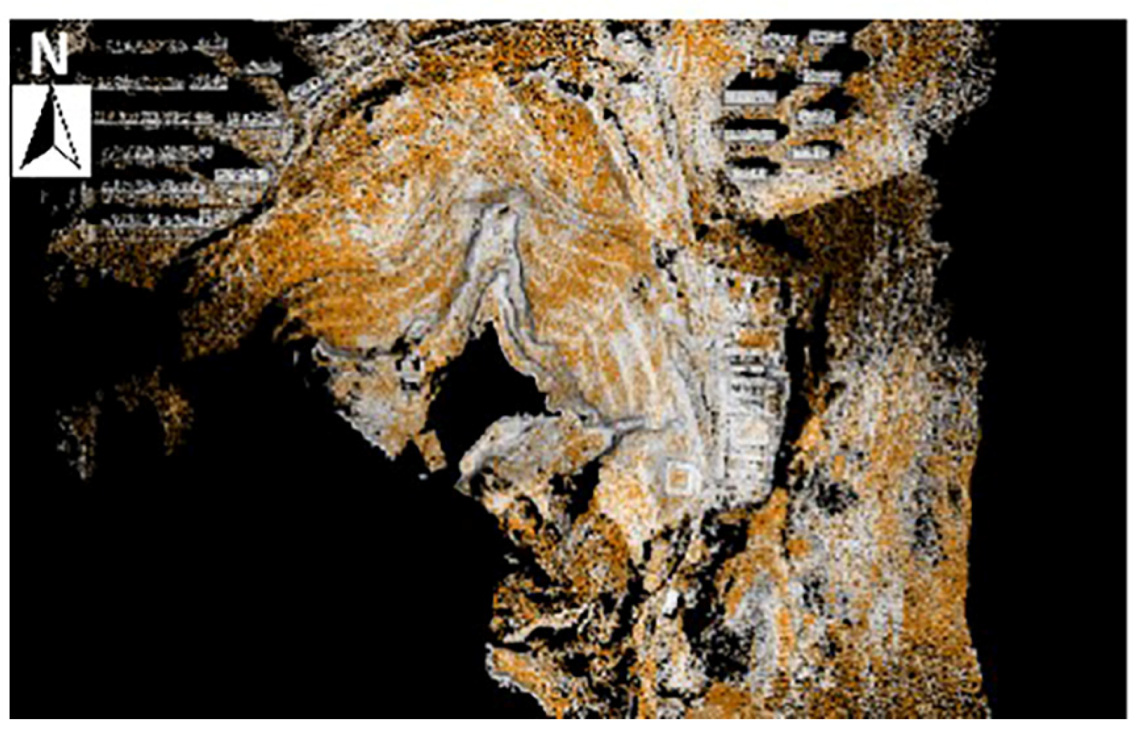
4.2.2. Geographic Information Extraction
5. Geographic Information Interpretation and Analysis
5.1. Identification of Geological Hazard Prone Areas
5.2. Slope Stability Analysis
5.3. Stability Analysis
6. Conclusions
- (1)
- UAV remote sensing technology is an efficient tool for identifying and monitoring geological hazards on slopes. The UAV is equipped with a multifunctional camera to capture high-definition images, and various surveying and mapping software are used to construct three-dimensional models. This approach enhances work efficiency and expands the monitoring scope compared to traditional methods of geological hazard monitoring.
- (2)
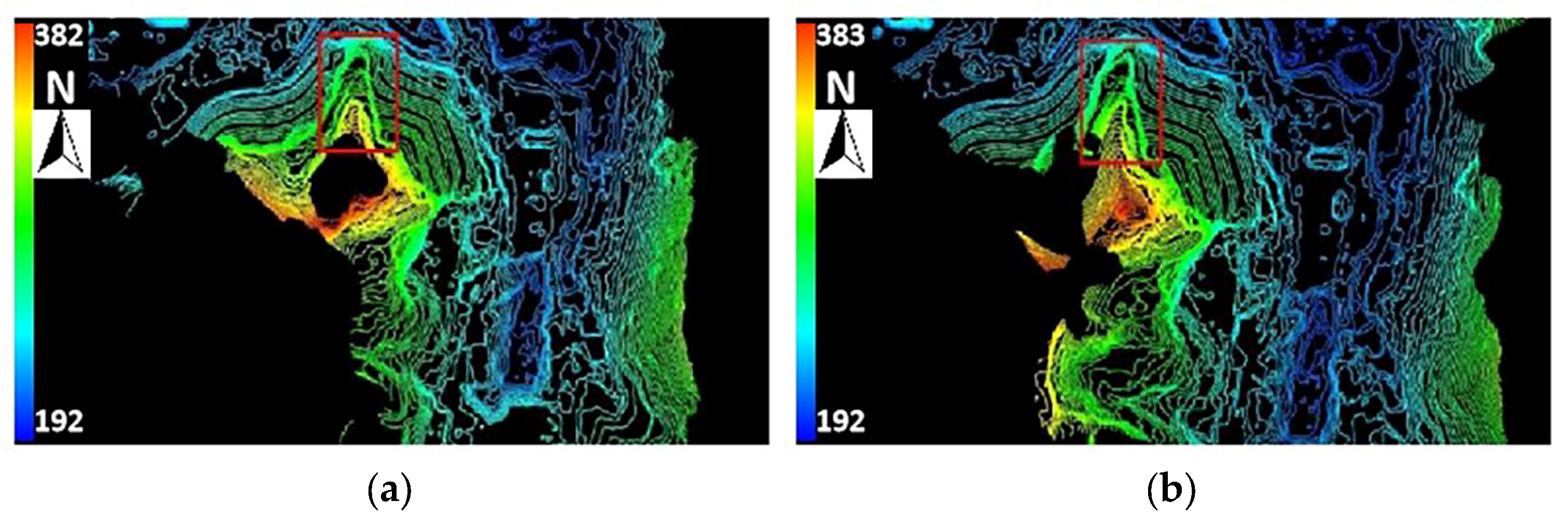
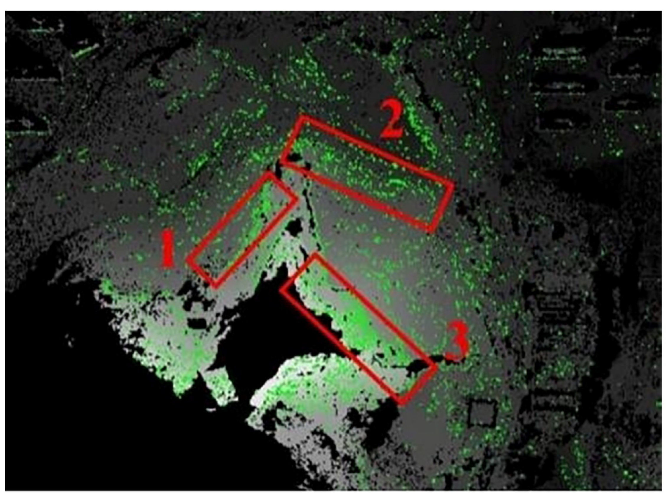
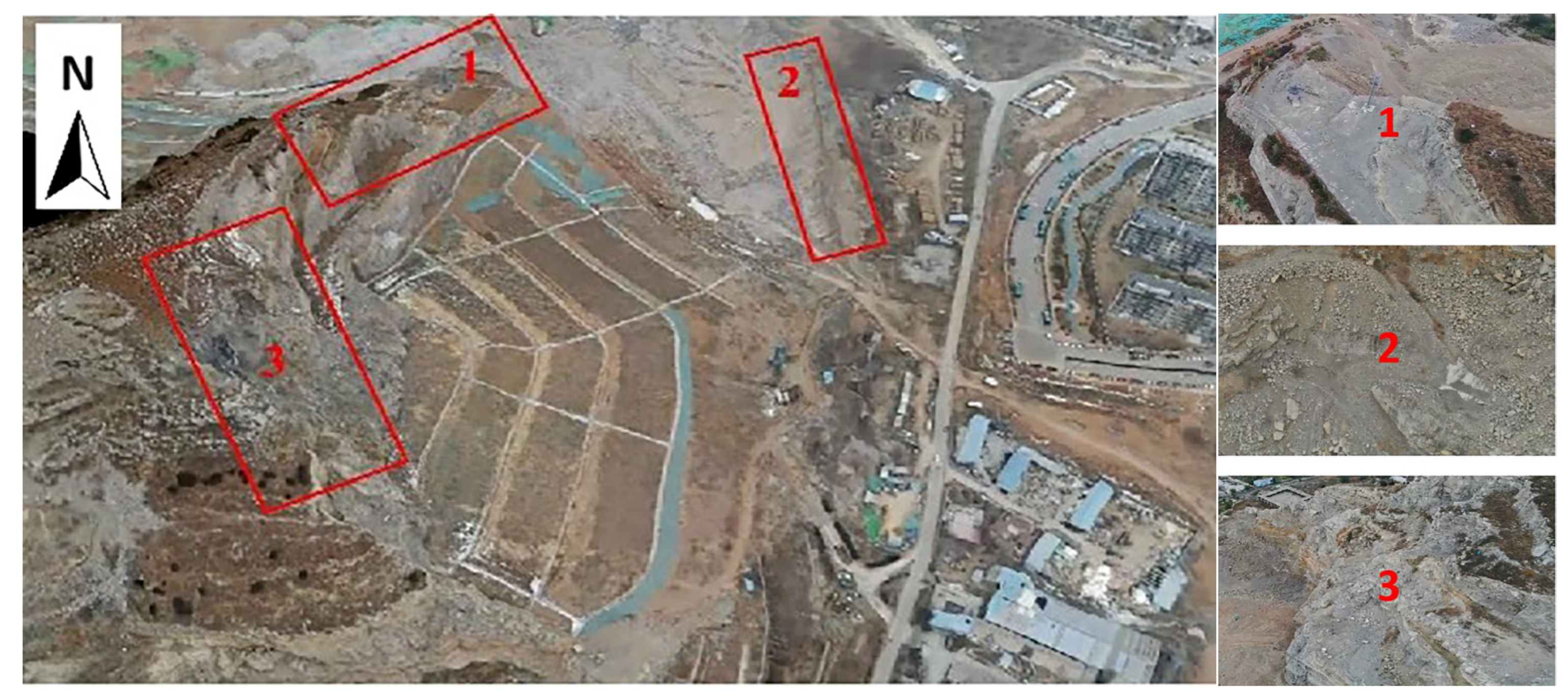
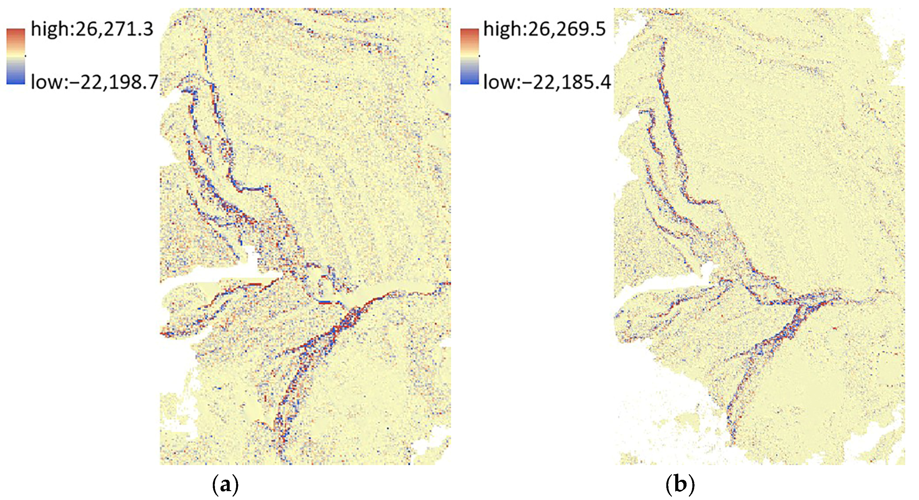
- Hazardous slope areas can be rapidly identified using the Digital Elevation Model, point-cloud model, and three-dimensional live model. By extracting the contour and point-cloud differential models of the study area and combining them with field investigation and analysis, two areas prone to geological hazards—susceptible to small debris avalanches and soil landslides—were identified.
- (3)
- Using the Digital Elevation Model to extract slope gradient and shape information, the stability of the two hazardous areas was analyzed. The maximum slope gradient in Areas 1 and 3 is approximately 87°, with many slopes exceeding 50°. The terrain is steep, and convex and concave slopes appear alternately, making the slope shape highly variable and prone to disasters. A stability evaluation was conducted using AHP and hazard calculation methods, and the slope’s stability status was determined. The slope’s stability status was determined, and it is recommended that greater attention be given to the area, with timely slope management to prevent harm to highways and people’s lives and property. This method is simple and practical, providing new approaches for slope stability assessment.
- (4)
- The proposed approach has broad applicability in areas such as slope change detection, slope engineering stability assessment, geological hazard identification, and road safety operation and maintenance management. It offers significant practical value by enhancing work efficiency, reducing labor costs, and improving the safety of both people and infrastructure.
Author Contributions
Funding
Institutional Review Board Statement
Informed Consent Statement
Data Availability Statement
Acknowledgments
Conflicts of Interest
Abbreviations
| UAV | Unmanned aerial vehicle |
| DEM | Digital elevation model |
| AHP | Analytic hierarchy process |
| RTK | Real-time kinematic |
| XML | ContextCapture blocks exchange |
| POS | Position and orientation system |
| ICP | Iterative closest point |
| IPTD | Improved progressive TIN densification |
| LAS | LASer file format |
References
- Wu, Y.; Tian, A.; Lan, H. Comparisons of Dynamic Landslide Models on GIS Platforms. Appl. Sci. 2022, 12, 3093. [Google Scholar] [CrossRef]
- Hussain, Y.; Schlogel, R.; Innocenti, A.; Hamza, O.; Iannucci, R.; Martino, S.; Havenith, H. Review on the Geophysical and UAV-Based Methods Applied to Landslides. Remote Sens. 2022, 14, 4564. [Google Scholar] [CrossRef]
- Mcdougall, S. 2014 Canadian Geotechnical Colloquium: Landslide runout analysis—Current practice and challenges. Can. Geotech. J. 2017, 54, 605–620. [Google Scholar] [CrossRef]
- Nigro, M.; Pierri, F.; Caccavale, F. Control of an Omnidirectional UAV for Transportation and Manipulation Tasks. Appl. Sci. 2021, 11, 10991. [Google Scholar] [CrossRef]
- Zhong, C.; Liu, Y.; Gao, P.; Chen, W.; Li, H.; Hou, Y.; Nuremanguli, T.; Ma, H. Landslide mapping with remote sensing: Challenges and opportunities. Int. J. Remote Sens. 2020, 41, 1555–1581. [Google Scholar] [CrossRef]
- Stott, E.; Williams, R.D.; Hoey, T.B. Ground Control Point Distribution for Accurate Kilometre-Scale Topographic Mapping Using an RTK-GNSS Unmanned Aerial Vehicle and SfM Photogrammetry. Drones 2020, 4, 55. [Google Scholar] [CrossRef]
- Zieher, T.; Toschi, I.; Remondino, F.; Rutzinger, M.; Kofler, C.; Mejia-Aguilar, A.; Schlögel, R. Sensor- and scene-guided integration of tls and photogrammetric point clouds for landslide monitoring. Int. Arch. Photogramm. Remote Sens. Spat. Inf. Sci. 2018, 42, 1243–1250. [Google Scholar] [CrossRef]
- An, S.; Yuan, L.; Xu, Y.; Wang, X.; Zhou, D. Ground subsidence monitoring in based on UAV-LiDAR technology: A case study of a mine in the Ordos, China. Geomech. Geophys. Geo-Energy Geo-Resour. 2024, 10, 57. [Google Scholar] [CrossRef]
- Qiu, H.; Zhai, H.; Wang, J.; Ge, S.; Wu, L. Geological survey and risk assessment based on UAV photogrammetry. Sci. Technol. Eng. 2024, 24, 7905–7912. (In Chinese) [Google Scholar]
- Wei, Y. Application of UAV Inclined Photogrammetry in Highway Survey and Design. Digit. Commun. World 2023, 101–103. (In Chinese) [Google Scholar] [CrossRef]
- Pi, H.; Peng, S.; Zeng, X. Expressway high slope monitoring information extraction using UAV oblique photogrammetry. Beijing Surv. Mapp. 2023, 37, 620–624. (In Chinese) [Google Scholar] [CrossRef]
- Zolkepli, M.F.; Ishak, M.F.; Talib, Z.A. Unmanned Aerial Vehicle (UAV)-Based for Slope Mapping and the Determination of Potential Slope Hazard. Int. J. Integr. Eng. 2022, 14, 232–239. [Google Scholar] [CrossRef]
- Yao, A.; Gong, Y.; Li, Y.; Tian, T.; Xu, C. Mountain-Expressway Slope Safety Based on the Online Monitoring System and Fuzzy Comprehensive Evaluation. J. Test. Eval. 2022, 50, 1906–1919. [Google Scholar] [CrossRef]
- Yang, Y.; Wu, W.; Zheng, H. Investigation of slope stability based on strength-reduction-based numerical manifold method and generalized plastic strain. Int. J. Rock Mech. Min. Sci. 2023, 164, 105358. [Google Scholar] [CrossRef]
- Zhang, Z.L.; Yang, X.L. Unified solution of safety factors for three-dimensional compound slopes considering local and global instability. Comput. Geotech. 2023, 155, 0266–0352X. [Google Scholar] [CrossRef]
- Liang, G.L.; Xu, W.Y.; He, Y.Z.; Zhao, Y.X. Application of catastrophe progression method to comprehensive evaluation of slope stability. Rock Soil Mech. 2008, 29, 1895–1899. [Google Scholar]
- Wang, S.; Zhang, Z.; Ren, Y.; Zhu, C. UAV Photogrammetry and AFSA-Elman Neural Network in Slopes Displacement Monitoring and Forecasting. KSCE J. Civ. Eng. 2020, 24, 19–29. [Google Scholar] [CrossRef]
- Huang, H.; Long, J.; Lin, H.; Zhang, L.; Yi, W.; Lei, B. Unmanned aerial vehicle based remote sensing method for monitoring a steep mountainous slope in the Three Gorges Reservoir, China. Earth Sci. Inform. 2017, 10, 287–301. [Google Scholar] [CrossRef]
- Wu, X.; Yang, Y.; Ye, Z. Stability of rock—Soil slopes under rainfall infiltration and its influencing factors. J. Water Resour. Water Eng. 2022, 33, 189–199. (In Chinese) [Google Scholar]
- Yuan, D.; Lu, J.; Liu, D.; Yang, Z.; Wang, J. Visual Query and Analysis System of Slope Monitoring Information and Its Application. J. Eng. Geol. 1999, 7, 355–360. (In Chinese) [Google Scholar]
- Li, P.; Wang, Q.; Li, J.; Pei, Y.; He, P. Automated extraction of tunnel leakage location and area from 3D laser scanning point clouds. Opt. Lasers Eng. 2024, 178, 108217. [Google Scholar] [CrossRef]
- Chen, Y.; Ye, Z.; Chen, Z.; Wang, G. Morphological deformation characteristics of landslide based on UAV imagery: Taking Xieliupo landslide in Bailong river basin of Longnan as an example. Seience Technol. Eng. 2024, 24, 2665–2672. (In Chinese) [Google Scholar]
- Kern, A.; Fanta-Jende, P.; Glira, P.; Bruckmüller, F.; Sulzbachner, C. An accurate real-time UAV mapping solution for the generation of orthomosaics and surface models. Int. Arch. Photogramm. Remote Sens. Spat. Inf. Sci. 2021, 43, 165–171. [Google Scholar] [CrossRef]
- Mir, S.; Shah, S.A.; Bhat, M.S.; Akhter, S.; Ahad, F.; Rashid, H.; Jeelani, P. Disaster risk assessment of educational infrastructure in mountain geographies using PROMETHEE-II. Int. J. Disaster Risk Reduct. 2024, 107, 104489. [Google Scholar] [CrossRef]
- Cirillo, D.; Zappa, M.; Tangari, A.C.; Brozzetti, F.; Ietto, F. Rockfall Analysis from UAV-Based Photogrammetry and 3D Models of a Cliff Area. Drones 2024, 8, 31. [Google Scholar] [CrossRef]
- Yu, H.; Li, Z.; Di, T.; Li, Y. Unmanned aerial vehicle images-based landslide geohazards interpretation and stability analysis: An illustrative example of Yanguan landslide. Sci. Technol. Eng. 2019, 19, 84–92. (In Chinese) [Google Scholar]
- Ruzic, I.; Benac, C.; Jovancevic, S.D.; Radisic, M. The Application of UAV for the Analysis of Geological Hazard in Krk Island, Croatia, Mediterranean Sea. Remote Sens. 2021, 13, 1790. [Google Scholar] [CrossRef]
- Wang, S.H.; Ahmed, Z.; Hashmi, M.Z.; Wang, P.Y. Cliff face rock slope stability analysis based on unmanned arial vehicle (UAV) photogrammetry. Geomech. Geophys. Geo-Energy Geo-Resour. 2019, 5, 333–344. [Google Scholar] [CrossRef]
- James, M.R.; Robson, S. Straightforward reconstruction of 3D surfaces and topography with a camera: Accuracy and geoscience application. J. Geophys. Res. Earth Surf. 2012, 117, 17. [Google Scholar] [CrossRef]
- Nex, F.; Remondino, F. UAV for 3D mapping applications: A review. Appl. Geomat. 2014, 6, 1–15. [Google Scholar] [CrossRef]
- Eltner, A.; Kaiser, A.; Castillo, C.; Rock, G.; Neugirg, F.; Abellan, A. Image-based surface reconstruction in geomorphometry—Merits, limits and developments. Earth Surf. Dyn. 2016, 4, 359–389. [Google Scholar] [CrossRef]
- Andrew, A.M. Multiple View Geometry in Computer Vision. Kybernetes 2001, 30, 1333–1341. [Google Scholar] [CrossRef]
- Zhang, J.; Lin, X. Filtering airborne LiDAR data by embedding smoothness-constrained segmentation in progressive TIN densification. ISPRS-J. Photogramm. Remote Sens. 2013, 81, 44–59. [Google Scholar] [CrossRef]
- Zhang, W.; Qi, J.; Wan, P.; Wang, H.; Xie, D.; Wang, X.; Yan, G. An Easy-to-Use Airborne LiDAR Data Filtering Method Based on Cloth Simulation. Remote Sens. 2016, 8, 501. [Google Scholar] [CrossRef]
- Meng, X.; Currit, N.; Zhao, K. Ground Filtering Algorithms for Airborne LiDAR Data: A Review of Critical Issues. Remote Sens. 2010, 2, 833–860. [Google Scholar] [CrossRef]
- Chen, Q.; Gong, P.; Baldocchi, D.; Xie, G. Filtering airborne laser scanning data with morphological methods. Photogramm. Eng. Remote Sens. 2007, 73, 175–185. [Google Scholar] [CrossRef]
- Reese, R.A. Geostatistics for Environmental Scientists. J. R. Stat. Soc. Ser. A-Stat. Soc. 2009, 172, 700. [Google Scholar] [CrossRef]
- Lu, G.Y.; Wong, D.W. An adaptive inverse-distance weighting spatial interpolation technique. Comput. Geosci. 2008, 34, 1044–1055. [Google Scholar] [CrossRef]
- Besl, P.J.; Mckay, N.D. A method for registration of 3-D shapes. IEEE Trans. Pattern Anal. Mach. Intell. 1992, 14, 239–256. [Google Scholar] [CrossRef]
- Rusinkiewicz, S.; Levoy, M. Efficient variants of the ICP algorithm. In Proceedings of the Third International Conference on 3-D Digital Imaging and Modeling, Quebec City, QC, Canada, 28 May–1 June 2001; pp. 145–152. [Google Scholar] [CrossRef]
- Chen, Y.; Medioni, G. Object modeling by registration of multiple range images. Image Vis. Comput. 1992, 10, 145–155. [Google Scholar] [CrossRef]
- Xue, Q.; Zhang, M.; Gao, B. Hazard assessment of loess landslide based on soil moisture content and supported by slope unit in Qingjian City, Shaanxi Province. Geol. China 2020, 47, 1904–1914. (In Chinese) [Google Scholar]
- Zevenbergen, L.W.; Thorne, C.R. Quantitative-analysis of land surface-topography. Earth Surf. Process. Landf. 1987, 12, 47–56. [Google Scholar] [CrossRef]
- Liu, J.; Wang, L. Investigation and Risk Assessment of a Loess Landslide Based on UAV Tilt Photogrammetry. Shuitu Baochi Tongbao 2023, 43, 139–147. [Google Scholar]
- Vandenberge, D.R.A.D.; Mcguire, M.P.A.M. Practical Use of Modified Hoek–Brown Criterion for Soil Slope Stability Analysis. Geotech. Geol. Eng. 2019, 37, 5441–5455. [Google Scholar] [CrossRef]
- Ni, K.; Yang, J.; Ning, Y.; Kang, G. A modified sub-block DDA fracturing modelling method for rock. Eng. Anal. Bound. Elem. 2020, 111, 154–166. [Google Scholar] [CrossRef]
- Kohno, M.; Ono, Y. Evaluation of earthquake-induced slope failure distribution using the AHP method and GIS. Int. J. GEOMATE 2021, 20, 74–81. [Google Scholar] [CrossRef]
- Ye, W.; Gao, C.; Liu, Z.; Wang, Q.; Su, W. A Fuzzy-AHP-based variable weight safety evaluation model for expansive soil slope. Nat. Hazards 2023, 119, 559–581. [Google Scholar] [CrossRef]
- Leong, E.C.; Rahardjo, H. Two and three-dimensional slope stability reanalyses of Bukit Batok slope. Comput. Geotech. 2012, 42, 81–88. [Google Scholar] [CrossRef]
- Vasquez, J.; Estrada, M. A comparative study of the bivariate statistical methods and the Analytical Hierarchical Process for the assessment of mass movement susceptibility. A case study: The LM-116 Road-Peru. Rud.-Geol.-Naft. Zb. 2023, 38, 149–166. [Google Scholar] [CrossRef]
- Cengiz, L.D.; Ercanoglu, M. A novel data-driven approach to pairwise comparisons in AHP using fuzzy relations and matrices for landslide susceptibility assessments. Environ. Earth Sci. 2022, 81, 222. [Google Scholar] [CrossRef]
- Abay, A.; Barbieri, G.; Woldearegay, K. GIS-based Landslide Susceptibility Evaluation Using Analytical Hierarchy Process (AHP) Approach: The Case of Tarmaber District, Ethiopia. Momona Ethiop. J. Sci. 2019, 11, 14–36. [Google Scholar] [CrossRef]
- He, H.; Hu, D.; Sun, Q.; Zhu, L.; Liu, Y. A Landslide Susceptibility Assessment Method Based on GIS Technology and an AHP-Weighted Information Content Method: A Case Study of Southern Anhui, China. ISPRS Int. J. Geo-Inf. 2019, 8, 266. [Google Scholar] [CrossRef]
- Saaty, T.L. A scaling method for priorities in hierarchical structures. J. Math. Psychol. 1977, 15, 234–281. [Google Scholar] [CrossRef]
- Vargas, L.G. An overview of the analytic hierarchy process and its applications. Eur. J. Oper. Res. 1990, 48, 2–8. [Google Scholar] [CrossRef]
- Zhang, L.; Wang, Y.; Zhang, J.; Zhang, S.; Guo, Q. Rockfall hazard assessment of the slope of Mogao Grottoes, China based on AHP, F-AHP and AHP-TOPSIS. Environ. Earth Sci. 2022, 81, 377. [Google Scholar] [CrossRef]
- Huang, J.L.; Zhao, J.G.; Zhang, T.; Li, J.L. AHP-based hazard degree assessment of high-speed landslide of reservoir bank. J. Nat. Disasters 2011, 20, 95–99. [Google Scholar]
- Shang, H.; Wang, Y.; Li, G.; Guo, Y.; Ma, A.; Yan, X.; Luo, Y. Research on Geological Environment Evaluation of Jinan Based on 3D Model. In Proceedings of the 3rd Guangdong-Hong Kong-Macao Greater Bay Area Artificial Intelligence and Big Data Forum, AIBDF 2023, Guangzhou, China, 22–24 September 2023. [Google Scholar]
- Zhu, M.; Li, L. Correlation Analysis of Geological Hazards and SoilRock Types in Taishan Scenic Area. Energy Technol. Manag. 2023, 48, 178–180. (In Chinese) [Google Scholar]


| Equipment Parameters | Norm |
|---|---|
| Weight (with battery) | 6.3 kg |
| Maximum horizontal flight speed | 23 m/s |
| Navigation system | GPS + GLONASS + BeiDou + Galileo |
| RTK position accuracy | 1.5 cm + 1 ppm (vertical); 1 cm + 1 ppm (horizontal) |
| Camera Pixels | Wide-angle 12 megapixels; Zoom 20 megapixels |
| Pitch of the head | Pitch: −120° to +30° Horizontal: ±320° |
| Maximum wind speed | 15 m/s |
| Maximum flight time per trip | 55 min |
| Parameter Classification | Parameter Name | Parametric Indicators |
|---|---|---|
| Image Information | Number of images | 74 |
| With positional image | 74 | |
| Calibrated images | 74 | |
| Root-mean-square error of geographic alignment | Phase I 0.957 m; Phase II 1.364 m | |
| times | airtime | Phase I 37 s; Phase II 53 s |
| RTK solution value | fixed solution | Phase I 74; Phase II 74 |
| floating solution | Phase I 0; Phase II 0 | |
| single-point solution | Phase I 0; Phase II 0 | |
| Other solutions | Phase I 0; Phase II 0 |
| A | B1 | B2 | B3 | B4 | WB |
|---|---|---|---|---|---|
| B1 | 1 | 3 | 5 | 7 | 0.513 |
| B2 | 1/3 | 1 | 3 | 5 | 0.289 |
| B3 | 1/5 | 1/3 | 1 | 3 | 0.135 |
| B4 | 1/7 | 1/5 | 1/3 | 1 | 0.054 |
| B | C1 | C2 | C3 | C4 | C5 | C6 | C7 | C8 | C9 | C10 | C11 |
|---|---|---|---|---|---|---|---|---|---|---|---|
| WC | 0.277 | 0.152 | 0.084 | 0.163 | 0.056 | 0.029 | 0.050 | 0.019 | 0.039 | 0.077 | 0.036 |
| Evaluation Projects | Classification of Indicators and Quantitative Scores Ci | ||
|---|---|---|---|
| 1 | 0.618 | 0.382 | |
| C1: Rock and Soil Type | loose stacked layer (geology) | semi-hard rock | solid bedrock |
| C2: Structural Plane Density | low density | Medium density | low density |
| C3: Weathering Degree | Strong weathering: weathering index > 0.6 | Medium weathering: 0.2 < weathering index ≤ 0.6 | Unweathered: weathering index ≤ 0.2 |
| C4: Slope Gradient | Steep slopes: slope > 30° | Medium gradient: 15–30° gradient | Gentle slopes: slopes < 15° |
| C5: Slope Aspect | downhill | transverse slope | reverse slope |
| C6: Curvature | convex slope | straight slope | concave slope |
| C7: Vegetation Coverage | Low coverage: <30% coverage | Medium coverage: 30–70% coverage | High coverage: >70% coverage |
| C8: Annual Average Rainfall | High rainfall areas: annual rainfall > 800 mm | Medium rainfall zone: annual rainfall 400–800 mm | Low rainfall zone: annual rainfall < 400 mm |
| C9: Groundwater Influence | Long-term saturation: water table depth < 3 m | Seasonal impact:3 m ≤ water level depth ≤ 5 m | No groundwater: depth to water table > 5 m |
| C10: Seismic Intensity | High intensity (>VII) | Medium intensity (degrees VI–VII) | Low intensity (<VI) |
| C11: Human-Induced Disturbance | Large-scale excavation: >30% of excavated area | Partial excavation: 10% ≤ excavated area ≤ 30% | Undisturbed: <10% of excavated area |
| C12: Vegetation Destruction Condition | Severe damage: recovery rate < 30% | Moderate damage: 30–60% recovery rate | Minor damage: recovery rate > 60% |
| i | 1 | 2 | 3 | 4 | 5 | 6 | 7 | 8 | 9 | 10 | 11 |
|---|---|---|---|---|---|---|---|---|---|---|---|
| 0.277 | 0.152 | 0.084 | 0.163 | 0.056 | 0.029 | 0.050 | 0.019 | 0.039 | 0.077 | 0.036 | |
| 0.382 | 0.382 | 0.618 | 1 | 0.618 | 0.382 | 1 | 0.618 | 0.382 | 0.618 | 1 | |
| 0.106 | 0.058 | 0.052 | 0.163 | 0.035 | 0.011 | 0.050 | 0.012 | 0.015 | 0.048 | 0.036 | |
| i | 1 | 2 | 3 | 4 | 5 | 6 | 7 | 8 | 9 | 10 | 11 |
Disclaimer/Publisher’s Note: The statements, opinions and data contained in all publications are solely those of the individual author(s) and contributor(s) and not of MDPI and/or the editor(s). MDPI and/or the editor(s) disclaim responsibility for any injury to people or property resulting from any ideas, methods, instructions or products referred to in the content. |
© 2025 by the authors. Licensee MDPI, Basel, Switzerland. This article is an open access article distributed under the terms and conditions of the Creative Commons Attribution (CC BY) license (https://creativecommons.org/licenses/by/4.0/).
Share and Cite
Li, N.; Qiu, H.; Zhai, H.; Chen, Y.; Wang, J. Monitoring and Analysis of Slope Geological Hazards Based on UAV Images. Appl. Sci. 2025, 15, 5482. https://doi.org/10.3390/app15105482
Li N, Qiu H, Zhai H, Chen Y, Wang J. Monitoring and Analysis of Slope Geological Hazards Based on UAV Images. Applied Sciences. 2025; 15(10):5482. https://doi.org/10.3390/app15105482
Chicago/Turabian StyleLi, Nan, Huanxiang Qiu, Hu Zhai, Yuhui Chen, and Jipeng Wang. 2025. "Monitoring and Analysis of Slope Geological Hazards Based on UAV Images" Applied Sciences 15, no. 10: 5482. https://doi.org/10.3390/app15105482
APA StyleLi, N., Qiu, H., Zhai, H., Chen, Y., & Wang, J. (2025). Monitoring and Analysis of Slope Geological Hazards Based on UAV Images. Applied Sciences, 15(10), 5482. https://doi.org/10.3390/app15105482