Article

High-Precision Positioning Method for Robot Acoustic Ranging Based on Self-Optimization of Base Stations

by
Zekai Zhang
1,
Jiayu Chen
1,
Bishu Gao
1,
Yefeng Sun
1,
Xiaofeng Ling
2,
Zheyuan Li
2 and
Liang Gong
1,*
1
School of Mechanical Engineering, Shanghai Jiao Tong University, Shanghai 200240, China
2
School of Information Science and Engineering, East China University of Science and Technology, Shanghai 200237, China
*
Author to whom correspondence should be addressed.
Appl. Sci. 2025, 15(10), 5478; https://doi.org/10.3390/app15105478
Submission received: 17 April 2025 / Revised: 9 May 2025 / Accepted: 12 May 2025 / Published: 13 May 2025

Abstract

:
In response to the demand for high-precision positioning within confined or indoor environments, the application of acoustic ranging methods has been widely adopted by numerous engineers. Currently, time-of-flight (TOF)-based acoustic ranging positioning systems face challenges such as the susceptibility of sound velocity to environmental factors and the loss of acoustic signals at both short and long distances, which leads to a reduction in positioning accuracy. This paper addresses these issues by proposing a high-precision confidence interval weighting method for acoustic ranging and further introduces a method for base station deployment and self-optimization positioning within fixed indoor base station scenarios. The method is based on trilateration positioning, establishing criteria for the division of central and boundary areas. It categorizes mobile terminal nodes based on their coordinates from the previous moment, selects distance information from nearby base stations in different modes, and employs weights for decision-making and computation, ultimately yielding two-dimensional positioning coordinates. Experiments demonstrate that the proposed method can effectively enhance the positioning accuracy of acoustic positioning systems compared to traditional four-base station weighted average positioning algorithms.

1. Introduction

In recent years, the field of autonomous driving algorithms has seen rapid development. To achieve effective control in autonomous vehicles, it is essential to first obtain the vehicle’s own attitude and position. To meet these positioning requirements, various methods such as GPS positioning, visual SLAM (simultaneous localization and mapping) positioning, UWB (ultra-wideband) positioning, and acoustic positioning have been continuously refined, each forming multiple positioning methods or integrated positioning algorithms.
GPS positioning and visual SLAM positioning methods are relatively expensive and have specific operational constraints. GPS positioning requires an unobstructed line of sight to the sky above the vehicle’s antenna to function properly, which limits its use in enclosed or urban environments. Visual SLAM, due to the processing speed of images, tends to have a lower frequency of positioning information, which can affect real-time performance.
UWB positioning, while requiring the installation of base stations, is generally more cost-effective and provides high-frequency positioning information with better real-time capabilities. However, the extremely fast propagation speed of electromagnetic waves can result in lower positioning accuracy, which may not meet the demands of high-precision applications.
In comparison, acoustic positioning also necessitates the setup of base stations, with costs similar to those of UWB positioning. The speed of sound is significantly lower than the speed of light, which allows for higher precision in signal transmission and reception. Therefore, acoustic positioning offers the advantages of low cost and high precision in small-scale scenarios, effectively meeting the positioning requirements.
Suolan Li et al. [1] proposed an improved SRP-PHAT [2] method for vehicle horn sound localization. By analyzing the sound, frequency domain features for identifying vehicle horn sounds were selected, and a corresponding time–frequency transform (VHSR-TFT)-based sound recognition method was proposed. Artem Sieriebriakov et al. [3] proposed an algorithm for determining the distance to a sound source based on estimating the variation in incoming sound power and frequency with distance. Through this algorithm, objects can be located solely based on their acoustic characteristics without requiring any visual information. Junling Wang et al. [4] used the phenomenon of sound diffraction to embed specific directional features into the emitted sound signal. After one-time calibration in the deployment environment, the system learns the directional signal, thereby achieving the positioning function of the mobile robot. However, the positioning accuracy of the above methods is difficult to break through to a positioning accuracy of ±5 cm. Therefore, this article aims to study how to stabilize the positioning accuracy within the range of ±5 cm.
This paper investigates the TOF method for ranging, which involves pre-estimating coordinates based on the distances from the base stations to the mobile terminal, thereby achieving positioning functionality. According to the principles of the TOF method, the measurement of time differences and the current speed of sound are key to enhancing ranging accuracy. In addition to this, after obtaining ranging information, it is necessary to perform coordinate calculations using an appropriate pre-estimation method. Focusing on the TOF ranging and positioning scenario with four base stations, this paper primarily explores how to reduce the errors in time difference measurements and how to select base stations and selectively choose ranging information for coordinate calculations.
This article mainly explains the above issues in Section 2 and Section 3. Section 2 describes the method of assigning high-precision confidence interval weights for acoustic ranging, while Section 3 discusses the deployment of base stations and self-optimization positioning methods, and it also presents experimental verification. Finally, Section 4 provides a summary and introduces future research directions.

2. High-Precision Confidence Interval Weight Assignment Method for Acoustic Ranging

2.1. Acoustic Localization Error Factors

Acoustic localization techniques based on the time-of-flight (TOF) [5,6,7] method primarily suffer from errors in two aspects of the ranging process, namely the measurement of transmission time and the calibration of the speed of sound. During the time difference measurement, the transmission time from the acoustic signal emitter to the receiver is composed of the propagation time of the acoustic signal through the air and the demodulation processing time after the signal is received. Due to potential obstructions or the inherent multipath effect along the shortest transmission path, the propagation time in the air may not be the minimum, leading to an overestimation of the measured distance. Additionally, as the amplitude of the acoustic wave decreases with increasing propagation distance, signal loss can occur at too great a distance, limiting the range of acoustic ranging. Conversely, when the distance between base station nodes is too short, the propagation distance of the acoustic wave is too brief, leading to signal loss at the receiving end; thus, acoustic ranging cannot be too close either. In summary, acoustic ranging errors increase rapidly when the distance is either too close or too far; only within an appropriate ranging confidence interval can the precision of acoustic ranging be ensured.
For the pre-estimation calculation method of coordinate positioning, three considerations are necessary. First, the distances measured must be at the same moment; second, the pre-estimation calculation method must be fast enough to ensure the timeliness of the coordinates; and third, the obtained distances must be of high precision and reliable. This paper discusses a scenario based on low-speed mobile terminals, which can be approximated as static coordinate estimation. Therefore, the primary focus of this paper is on the high-precision confidence interval of acoustic ranging and how the positioning algorithm ensures that the obtained coordinates are of high precision and reliably accurate.

2.2. Preprocessing Methods for Sound Signals

To achieve noise reduction and mitigate the effects of multipath propagation, acoustic signals generally require modulation. The receiving end can then demodulate and obtain the required transmission time information through methods such as the cross-correlation (CC) method.
However, in actual acoustic fields, factors such as noise and reverberation can cause ambiguity in the cross-correlation function, weakening the maximum peak and introducing spurious peaks, which complicates peak detection. To sharpen the peak, a certain weight can be added to the cross-power spectrum in the frequency domain, and then an inverse transformation can be applied to obtain the generalized cross-correlation function in the time domain. The transmission time is calculated based on the generalized cross-correlation function, which is known as the generalized cross-correlation (GCC) method.
By preprocessing acoustic signals with the generalized cross-correlation (GCC) method, it is acknowledged that ultrasonic waves attenuate continuously as they propagate through the air. Therefore, when the distance is too great, the acoustic signal may not be correctly received or recognized; conversely, when the distance is too close, due to the beam radiation characteristics of the sound waves, receivers outside the half-diffraction angle will also fail to correctly receive the acoustic signals. Consequently, to maintain high-precision ranging results, acoustic ranging methods must operate within an appropriate ranging confidence interval to ensure that the ranging information is of high precision.

2.3. High-Precision Confidence Interval Weight Assignment Method

To establish a high-precision confidence interval for acoustic ranging and to assign the necessary weights for subsequent positioning, this study employs two base station nodes, starting from a distance of 5 cm between them and incrementally increasing this distance until the absolute error in the measured range becomes significantly larger, at which point the distance increment is halted. The results obtained are depicted in Figure 1.
Upon examining the curve fitted by the least squares method, an error threshold of y = 0.03 m is adopted as the boundary for the high-precision positioning interval. The intersection points of y = 0.03 m with the leftmost and rightmost points of the error curve are determined to be xa = 2.834 m and xb = 20.153 m, respectively.
Based on the obtained values of xa and xb, a formula for the weights within the high-precision ranging confidence interval is constructed. From the curve in Figure 1, it can be seen that as the distance decreases at close range, the error will rapidly increase, while as the distance increases at long range, the error will slowly increase. At the same time, the larger the error, the lower the credibility weight. Therefore, in order to meet the above two characteristics, exponential functions are used as the main body at both close and long distances. In summary, to ensure the continuity of weight assignment, the formula for calculating the weight p is as follows:
p = f x = e x 1 e x a 1   , 0 < x < x a   1   , x a x x b e l n 2 x x b x a   , x > x b
In Equation (1), x is the ranging distance and xa and xb can be obtained from Figure 1.
When setting up this piecewise function, the following three characteristics are satisfied: the weight value is 0 when the distance is 0; the weight at the boundary between xa and xb is 1, maintaining continuity; and when the distance is greater than xb and less than xa, the change in distance will cause the error to increase rapidly, so an exponential function is used.
The coefficient before x can be modified according to the actual sound distance measurement error curve of the scene. The weights will serve as the basis for the base station’s self-optimization trilateration positioning method, thereby enhancing the accuracy of the final two-dimensional coordinates.

3. Base Station Deployment and Self-Optimization Positioning Method

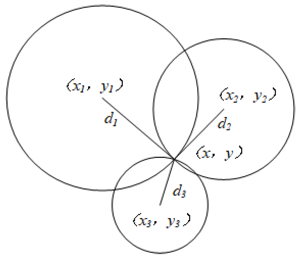
3.1. Trilateration Positioning

Based on various sensors, numerous positioning technologies have been developed to date, such as GPS positioning [8], visual SLAM positioning [9], UWB positioning [10], and acoustic positioning [11]. On the geometric algorithm level, there are currently methods such as trilateration algorithms, maximum–minimum algorithms, and maximum likelihood algorithms [12]. Due to the low computational complexity and relatively good positioning accuracy of the trilateration positioning algorithm, this paper adopts the trilateration positioning algorithm to calculate the coordinate information of the mobile terminal.
The trilateration positioning algorithm is an algorithm based on geometric principles. It performs positioning calculations based on the distances from at least three known coordinate nodes to the target node. The principle is illustrated in Figure 2.
Assuming there are three nodes with known coordinate information distributed across the map, their coordinates are denoted as (x1, y1), (x2, y2), and (x3, y3). Let the coordinate information of the target node be (x, y). The distances from the target node to each of the known nodes are
d i = x x i 2 + y y i 2
Circles are drawn with the known nodes as centers and the distances from the target node to the known nodes as radii. In theory, the three circles should intersect at a single point, which is the coordinate of the target node.
The equation for the trilateration algorithm is
x x 1 2 + y y 1 2 = d 1 2 x x 2 2 + y y 2 2 = d 2 2 x x 3 2 + y y 3 2 = d 3 2
By transforming and converting Equation (3) to obtain Equation (4), the coordinate information of the target node (x, y) can be directly solved for
x y = 2 x 1 x 3 2 y 1 y 3 2 x 2 x 3 2 y 1 y 3 1 x 1 2 x 3 2 + y 1 2 y 3 2 + d 3 2 d 1 2 x 2 2 x 3 2 + y 2 2 y 3 2 + d 3 2 d 2 2
However, it can be anticipated that in most cases, due to the inaccuracy of ranging results, the three circles may not intersect or they may intersect to form a closed area [13], leading to poor positioning accuracy. To address this issue, Zhou Yu et al. [14] proposed an N-times trilateral centroid weighted localization algorithm (NTCWALA). This method involves multiple measurements of the same target coordinates, assigning weights to the measured coordinates each time and then using the weighted average to filter out target coordinates that differ significantly from the weighted average. Finally, a weighted average is taken of the remaining target coordinates, which is used as the coordinate of the target node. This method improves positioning accuracy at the expense of increased time. Fang Huanyang et al. [15] used the Fang algorithm to determine the coordinates of the positioning target, but the Fang algorithm, which has an analytical solution, is prone to producing dual solutions, and its positioning accuracy significantly decreases when there is a large error in a measurement value. Bao Jianjun et al. [16] used the least squares positioning algorithm to determine the position of the positioning target, which is simple to implement but tends to yield suboptimal solutions with room for improvement in accuracy. Minghao Z et al. [17] suggested that increasing the number of measurement nodes can improve the precision of ranging measurements, but this would correspondingly increase costs.
This paper, based on the principles of the trilateration positioning algorithm, primarily explores how to select distance information with relatively higher precision through a base station self-optimization method when four known nodes’ distances to the target node are obtained, in order to perform positioning calculations and achieve higher precision in the positioning coordinates.

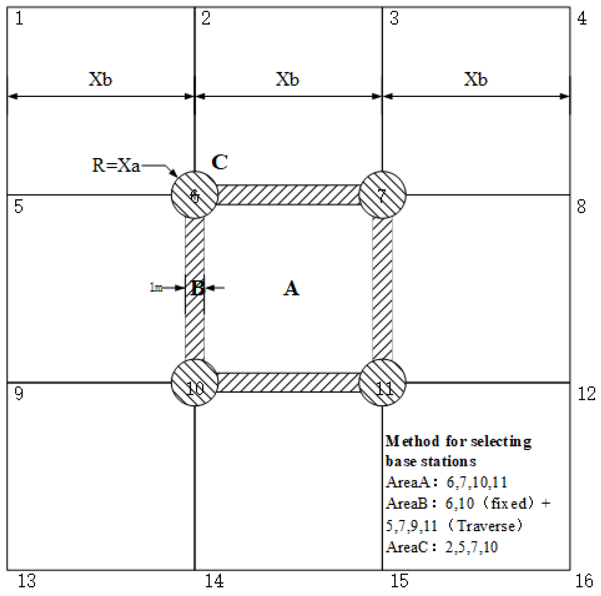
3.2. Base Station Deployment and Transition Zone Division Method

In large-scale scenarios, due to the limited high-precision ranging distance of a single base station, a substantial number of fixed base station nodes needs to be deployed with rational spacing and configuration to ensure the positioning accuracy of two-dimensional coordinates. This paper adopts a square grid with a side length of xb for the extensive deployment of base stations.
When the mobile beacon operates near the boundary of the square area, on one hand, the accuracy weight of the two-dimensional positioning coordinates obtained through the base station’s self-optimization method is relatively low. On the other hand, a basis for determining the mobile beacon’s transition to an adjacent area has not yet been established. This paper divides the boundary of the square area into a transitional zone between two adjacent areas and establishes a special method for the optimal selection of base stations within the transitional zone. The division of the transitional zone is shown in Figure 3.
The division results are depicted in Figure 3, which are divided into an A-type central area, B-type transition area, and C-type transition area. By establishing transition areas and a central area in this manner, the impact of lower accuracy in short-range ranging can be effectively mitigated. Additionally, it facilitates the selection and switching of base stations when crossing regions, thereby effectively enhancing the positioning accuracy in the transition areas and achieving the goal of high-precision positioning coverage across the entire map.

3.3. Self-Optimization Positioning Method for Base Stations

According to the trilateration positioning algorithm, it is evident that the distance information from three known coordinate nodes to the target node is sufficient to determine the coordinates of the target node. However, as explored in Section 2, when the mobile terminal is too close to or too far from the base station node, the absolute error in the measured distance information is relatively large. According to the regional division in Section 3.2, the base station self-optimization is specifically divided into three modes. When calculating the positioning coordinates, the selection of the base station self-optimization mode is based on the positioning coordinates from the previous moment.

3.3.1. A-Type Central Area

Taking Figure 3 as an example, the A-type central area selects base station nodes 6, 7, 10, and 11 as the basis for distance measurement information in positioning. Facing the distances d1, d2, d3, and d4 from four known coordinate base station nodes to the target mobile terminal, this paper assigns weights to each distance measurement information based on the weighting formula from Section 2, with weights denoted as p1, p2, p3, and p4.
In the selection of distance measurement information, the first choice is the distance information with a weight greater than or equal to 0.5. However, within the square positioning area with side length xb, it is not possible to find three reliable high-precision distance measurements with weights greater than 0.5 at every location. Three specific scenarios are as follows:
(1)
There are four distance measurements with weights greater than or equal to 0.5;
(2)
There are only three distance measurements with weights greater than or equal to 0.5;
(3)
There are only two distance measurements with weights greater than or equal to 0.5.
Due to the division of transition areas, there will be no distance measurements in the Type A central area with a distance less than xa; thus, only the first and second scenarios need to be considered.
In the first scenario, this paper adopts a weighted average approach. By selecting any three out of the four distance measurements for permutation and combination positioning, four positioning coordinates (x1, y1), (x2, y2), (x3, y3), and (x4, y4) can be obtained. Simultaneously, the weights q1, q2, q3, and q4 for the four positioning coordinates are assigned according to the following formula:
q i = p j + p m + p n 3
In Equation (5), pj, pm, and pn represent the weights of the three distance measurements used in the calculation of the i-th coordinate.
After obtaining the weights for each coordinate, the final positioning coordinates are determined using the weighted average formula as follows:
x i ,     y i = q i x i ,     q i y i q i
For the second scenario, distance measurements with weights less than 0.5 are directly discarded, and the three distance measurements with weights greater than or equal to 0.5 are selected to calculate the two-dimensional coordinates.

3.3.2. B-Type Transition Area

Taking Figure 3 as an example, when the coordinates from the previous moment are within the B-type transition area, the two nodes at the ends of the current boundary, namely nodes labeled 6 and 7, are fixedly selected. Concurrently, the four nearby base station nodes, namely nodes labeled 2, 3, 10, and 11, are iterated through to serve as the third ranging node. This process yields four positioning coordinates with associated weights. During the iteration, if a ranging measurement with a weight less than 0.5 is encountered, the positioning coordinate obtained from that measurement is immediately discarded. Ultimately, the weighted average Equation (6) is applied to derive the final positioning coordinates.

3.3.3. C-Type Transition Area

Taking Figure 3 as an example, when the coordinates from the previous moment are within the C-type transition area, that is, within the radius xa of a certain base station node, the four closest base station nodes to that base station node are selected, namely nodes labeled 2, 5, 7, and 10. By permuting and combining these, four positioning coordinates with associated weights can be obtained. Finally, the weighted average Formula (6) is applied to calculate the final positioning coordinates.

3.3.4. Judgment Logic

According to the code displayed in Algorithm 1, the current moment’s ranging information dd and the previous moment’s coordinates pointt−1 are inputted as the basis for determining which area the current location is in. Initially, it is checked whether the shortest ranging distance d_min to the current moment’s coordinates is less than xa. If so, it is determined that the location is within the C-type transition area, and the AreaC function is called. If not, the dist function is called to first identify the coordinates of the two base station nodes corresponding to the shortest ranging distance at the current moment. Based on the previous moment’s coordinates pointt−1 (xt−1, yt−1), the perpendicular distance dis to the line connecting the two base station nodes is calculated. If the distance dis is less than 0.5 m, it is determined that the location is within the B-type transition area, and the AreaB function is called. Otherwise, it is determined that the location is within the A-type central area, and the AreaA function is called. After determining the area, subsequent weighted average coordinate calculations are carried out according to the procedures specific to each area.
Algorithm 1 Base station self optimization algorithm
1:Input: Distance set d, Time t−1 coordinate set pointt−1
2:Output: Time t coordinate set pointt
3:  d_min ← min(d)
4:  If d_min < xa
5:     AreaC;
6:  else
7:     Dis ← dist(d, pointt−1)
8:     If dis < 0.5
9:     AreaB;
10:     else
11:     AreaA;
12:     End if
13:  End if
In terms of algorithm complexity, this algorithm only adds classification judgment; thus, compared to traditional algorithms, the time complexity has not changed, and it can also meet computing power requirements with common hardware.

3.4. Experiment and Results

3.4.1. Simulation Experiment on Positioning Accuracy of A-Type Central Area

In accordance with the base station self-optimization trilateration positioning method, this paper conducts experimental validation through simulation. To verify the accuracy of the weighted average positioning coordinate calculation method under the new weight assignment method, this paper utilizes data recorded from a circuit around the peripheral areas within a 12 m × 20 m venue as the true values for positioning coordinates in the simulation experiment. During the experiment, a uniformly distributed random ranging error of [0, 0.03 m] is added to each ranging information point, serving as the input for the ranging distance in the base station self-optimization positioning algorithm. Ultimately, the positioning coordinates were obtained based on the self-optimization positioning algorithm described in Section 3.3. The results are shown in Figure 4.
As depicted in Figure 4, the mean error of the new base station self-optimization positioning algorithm is only 3.40576 cm, with a variance of 0.0412677 m2, achieving a positioning accuracy at the centimeter level and exhibiting good stability. Observing the overall trajectory, the positioning path is not smooth, indicating the presence of certain jitter errors, suggesting that there is still room for improvement in the algorithm.

3.4.2. Cross-Regional Positioning Accuracy Comparison Experiment

Traditional weighted average positioning algorithms do not incorporate regional selection distinctions. To validate that the precision of the transition zone-based base station self-optimization positioning method surpasses that of the traditional weighted average positioning algorithms, the ranging information dt is generated with errors based on the true value d using the following formula during simulation:
d t = d + r × e 0.1 × d x a   , 0 < x < x a   d + r × 0.03   , x a x x b   d + r × 0.03 + 0.05 × d x b   , x > x b
In the equation, r is a uniformly distributed random number within the range [−1 m, 1 m]. If the generated error is less than 0, then the error is taken as r × xa. Although noise in real-world scenarios is more in line with Gaussian noise models, in order to better compare the differences in positioning accuracy between the two methods, this paper uses a uniform distribution noise model to test the positioning accuracy performance of different methods in harsh site environments. But as a result, some cases with extremely large errors in the Gaussian distribution model will also be lost. However, based on Equation (1) mentioned earlier, when the distance measurement information is clearly unreasonable and the weight value is very small, it will be directly discarded and not applied to the positioning algorithm. Therefore, using a uniformly distributed noise model also has some rationality.
Subsequently, 100 straight paths with lengths greater than 1.75xb are randomly generated within the central 2xb × 2xb area of a 3xb × 3xb venue. Trilateration positioning calculations are performed using both the traditional algorithm and the novel base station self-optimization positioning algorithm, and the mathematical expectations and variances of the errors are compared. The results are shown in Figure 5.
From Figure 5, it can be observed that the mathematical expectation and variance of the base station self-optimization positioning method based on transition zone division are significantly lower than those of the traditional weighted average positioning algorithm. This indicates that the novel base station self-optimization positioning algorithm effectively enhances the precision and stability of positioning. By appropriately selecting base stations, avoiding the use of ranging information from short distances and discarding unreliable ranging information with weights less than 0.5, the base station self-optimization positioning method based on transition zone division effectively improves positioning accuracy and stability. Furthermore, it ensures a smoother transition in base station selection for mobile terminal nodes when crossing different areas.

4. Conclusions

Addressing the high-precision positioning requirements for small-scale or indoor scenarios, this paper proposes a transition zone-based base station self-optimization method for high-precision acoustic ranging in robotic applications. Acoustic signals are susceptible to environmental factors such as temperature, humidity, and airflow, leading to significant absolute errors in both short-range and long-range transmission. To enhance the precision of the distance information obtained after preprocessing, this paper establishes a high-precision confidence interval for ranging information and introduces a novel method for assigning weights within the high-precision acoustic ranging confidence interval. Furthermore, to achieve positioning functionality, this paper presents a weighted average-based self-optimization positioning method based on the trilateration algorithm. This method selects ranging information with higher precision from the confidence interval as input for the positioning algorithm and calculates the weighted average based on the assigned weights, thereby improving the positioning accuracy of two-dimensional coordinates and facilitating the transition of base station selection modes across different areas. Experimental validation has confirmed that the acoustic signal positioning method realized by the aforementioned approach achieves centimeter-level precision, meeting the requirements for practical scenario applications.
However, although this positioning method can improve positioning accuracy, it cannot meet the typical positioning update frequency (≥10 Hz) of current real-time robot navigation and can only achieve an update frequency of 2–5 Hz. In the future, we will consider adding UWB positioning components to integrate the advantages of fast UWB positioning update frequency, high acoustic positioning accuracy, and IMU local supplementary positioning to develop a multi-sensor fusion positioning module. The UWB update frequency can easily reach 50 Hz, but due to its propagation at the speed of light, the measurement accuracy of propagation time is difficult to guarantee, resulting in difficulty in breaking through the positioning accuracy to within ±10 cm. Therefore, the subsequent multi-sensor fusion methods consider UWB positioning as the main body and acoustic positioning with low-frequency correction assistance to achieve high-frequency and high-precision indoor positioning.

Author Contributions

Methodology, Z.Z., X.L. and L.G.; software, Z.L.; validation, Z.Z. and Z.L.; formal analysis, Z.Z. and J.C.; investigation, Y.S. and B.G.; data curation, Z.Z. and Z.L.; writing—original draft preparation, Z.Z.; writing—review and editing, Z.Z. and L.G.; supervision, L.G.; project administration, L.G. All authors have read and agreed to the published version of the manuscript.

Funding

The work is supported by the Shanghai Agriculture Applied Technology Development Program, China (grant no. T2022-03-01).

Institutional Review Board Statement

Not applicable.

Informed Consent Statement

Not applicable.

Data Availability Statement

The original contributions presented in this study are included in the article. Further inquiries can be directed to the corresponding author.

Conflicts of Interest

The authors declare that they have no known competing financial interests or personal relationships that could have appeared to influence the work reported in this paper.

Abbreviations

The following abbreviations are used in this manuscript:
TOFTime of Flight
GPSGlobal Positioning System
UWBUltra-Wide Band
SLAMSimultaneous Localization and Mapping
GCCGeneralized Cross-Correlation
CCCross-Correlation
TDOATime Difference in Arrival

References

  1. Li, S.; Chang, X.; Yang, C.; Jiang, K.; Wang, Z.; Wang, L.; Li, X. A Fast Vehicle Horn Sound Location Method with Improved SRP-PHAT. In Proceedings of the 2018 IEEE International Conference on Progress in Informatics and Computing (PIC), Suzhou, China, 14–16 December 2018. [Google Scholar]
  2. Dibiase, J.H. A High-Accuracy, Low-Latency Technique for Talker Localization in Reverberant Environments. Ph.D. Thesis, Brown University, Providence, RI, USA, 2000. [Google Scholar]
  3. Sieriebriakov, A.; Hospodarchuk, O.; Lakhtyr, D.; Simakhin, V.; Bondar, S. Technology of sound source localization based on incoming sound intensity. In Proceedings of the 2023 IEEE 18th International Conference on Computer Science and Information Technologies (CSIT), Lviv, Ukraine, 19–21 October 2023. [Google Scholar]
  4. Wang, J.; Guo, Y.; Lu, S.; Zhang, Y.; Shu, H. An Acoustic Indoor Localization Method Based on Directional Variability for Mobile Robot. In Proceedings of the 2024 IEEE International Conference on Industrial Technology (ICIT), Bristol, UK, 25–27 March 2024. [Google Scholar]
  5. Wu, S.; Zhang, S.; Huang, D. A TOA-Based Localization Algorithm With Simultaneous NLOS Mitigation and Synchronization Error Elimination. IEEE Sens. Lett. 2019, 3, 1–4. [Google Scholar] [CrossRef]
  6. Tong, K.; Wang, X.; Khabbazibasmenj, A.; Dounavis, A. Optimum reference node deployment for TOA-based localization. In Proceedings of the 2015 IEEE International Conference on Communications (ICC), London, UK, 8–12 June 2015. [Google Scholar]
  7. Zhu, K.; Wei, Y.; Xu, R. TOA-based localization error modeling of distributed MIMO radar for positioning accuracy enhancement. In Proceedings of the 2016 CIE International Conference on Radar (RADAR), Guangzhou, China, 10–13 October 2016. [Google Scholar]
  8. Koohzadi, M.; Ebadollahi, S.; Vahidnia, R.; Dian, F.J. Implementation and Comparison of Different Tropospheric Models to Reduce Error Low-cost Real-time GPS Positioning. In Proceedings of the 2019 IEEE 10th Annual Information Technology, Electronics and Mobile Communication Conference (IEMCON), Vancouver, BC, Canada, 17–19 October 2019. [Google Scholar]
  9. Yan, Z.; Wan-Fang, Z.; Li-Li, C. Design of Robot Positioning System Based on the Integration of Slam System and Inertial System. In Proceedings of the 2022 International Conference on Intelligent Transportation, Big Data & Smart City (ICITBS), Hengyang, China, 26–27 March 2022. [Google Scholar]
  10. Wu, F.; Liu, Z. Research on UWB/IMU Fusion Positioning Technology in Mine. In Proceedings of the 2020 International Conference on Intelligent Transportation, Big Data & Smart City (ICITBS), Vientiane, Laos, 11–12 January 2020. [Google Scholar]
  11. Zhang, Z.; Han, X.; Shi, Y.; Wang, Y.; Ma, L.; Yin, J. Acoustic Positioning System Beneath the Arctic Ice and Its Experimental Verification. In Proceedings of the 2024 OES China Ocean Acoustics (COA), Harbin, China, 29–31 May 2024. [Google Scholar]
  12. Goldoni, E.; Savioli, A.; Risi, M.; Gamba, P. Experimental analysis of RSSI-based indoor localization with IEEE 802.15.4. In Proceedings of the 2010 European Wireless Conference (EW), Lucca, Italy, 12–15 April 2010. [Google Scholar]
  13. Banda, S.; Hemanth, K.; Karanam Uma Maheshwar, R. A robust approach for WSN localization for underground coal mine monitoring using improved RSSI technique. Math. Model. Eng. Probl. 2018, 5, 225–231. [Google Scholar]
  14. Zhou, Y.; Qiu, T.; Xia, F.; Hou, G. N-Times Trilateral Centroid Weighted Localization Algorithm of Wireless Sensor Networks. In Proceedings of the Internet of Things (iThings/CPSCom), 2011 International Conference on and 4th International Conference on Cyber, Physical and Social Computing, Dalian, China, 19–22 October 2011. [Google Scholar]
  15. Fang, H.; Li, Y. Wireless Basestation Location Algorithm based on Clustering and TDOA. Commun. Technol. 2019, 311–317. [Google Scholar] [CrossRef]
  16. Bao, J.; Huo, Z.; Xu, W.; Zhao, Y. A Wireless Location Method with High Precision for Underground Personnel Tracking. Ind. Mine Autom. 2009, 10, 18–21. [Google Scholar]
  17. Zu, M.; Rong, X. UWB Indoor Localization Algorithm Based on Inner Triangle Centroid Correction and Taylor. Nat. Sci. J. Harbin Norm. Univ. 2018, 42–47. [Google Scholar] [CrossRef]
Figure 1. Curve of acoustic distance measurement error with distance variation.
Applsci 15 05478 g001
Figure 2. Trilateration positioning principle.
Applsci 15 05478 g002
Figure 3. Area division.
Applsci 15 05478 g003
Figure 4. Simulation results of self-optimizing positioning algorithm for base stations.
Applsci 15 05478 g004
Figure 5. Comparison experiment results of cross-regional positioning accuracy.
Applsci 15 05478 g005
Disclaimer/Publisher’s Note: The statements, opinions and data contained in all publications are solely those of the individual author(s) and contributor(s) and not of MDPI and/or the editor(s). MDPI and/or the editor(s) disclaim responsibility for any injury to people or property resulting from any ideas, methods, instructions or products referred to in the content.

