Modeling and Analysis of Dynamics of Rigid–Flexible Coupled Parallel Robots

Abstract

Rigid–flexible coupled robots have problems such as vibration and elastic deformation caused by the flexibility of the members during the motion process, which significantly impacts the system’s motion accuracy and dynamics performance. To address the above problems, a dynamic modeling method based on a vector bond graph is proposed, and a multi-energy domain global dynamic model of Delta-type rigid–flexible coupled parallel robot considering rod flexibility is established. The coupled vibration of the control part and mechanical part of the system is analyzed, and model simulation is verified by 20-sim 4.4 software and ADAMS software (instructional version), which verifies the validity and reasonableness of the modeling method and provides a reference for the modeling of other rigid–flexible coupled systems with parallel systems in space.

1. Introduction

Traditional robots are connected by rigid connecting rods with large motion inertia, which can only realize low motion speed and acceleration, thus affecting work efficiency. With the continuous development of modern machinery in the direction of lightweight, low energy consumption, and high efficiency, rigid–flexible coupled robots with increased member flexibility or flexible members replacing rigid members are becoming increasingly widely used [1]. However, the vibration and elastic deformation caused by component flexibility can affect the motion accuracy and dynamics of the system, which has become the focus of the current research on this type of rigid–flexible coupled robot [2,3,4,5].

Rigid–flexible coupled robots are mainly divided into tandem and parallel robots, among which the dynamics modeling problem of rigid–flexible coupled parallel robots has been a hot research topic in recent years [6,7]. Kang et al. [8,9] established the dynamics model of planar flexible parallel robots using the hypothetical modal method and illustrated the effect of the vibration of the flexible rod on the dynamics of the whole flexible robot system. Briot et al. [10] constructed a dynamic model of a flexible planar parallel robot by combining Newton–Euler’s principle with the principle of virtual work. Sun et al. [11] used D’Alembert’s principle to build a dynamics model of a spatial Delta-S rigid–flexible coupled parallel robot and performed a dynamic static analysis. Yu et al. [12,13] constructed a dynamic model of a planar 3-RRR flexible parallel robot and flexible robot containing flexible hinges. Other modeling methods include the Kineto-Elastodynamics (KED) method, the finite element method, and the concentrated mass method [14,15,16]. The above literature shows that most of the modeling and experimental studies have been conducted for planar flexible parallel robots, while the studies for spatial flexible parallel robots are fewer and limited to systems with a single energy domain.

Power bond graph is a system dynamics modeling method [17]. Yazman et al. [18] proposed a method for modeling the dynamics of flexible multibody systems based on the hypothetical modal method and bond graph theory and constructed a Euler–Bernoulli beam bond graph model. Damić et al. [19] pointed out that flexible robotic systems are both rigid–flexible coupled and multi-energy-domain physical systems and established a bond graph model of a 2-dimensional finite element beam structure, and analyzed the dynamic response. These studies provide a reasonable paradigm for developing models for such multi-energy domain systems. However, the power bond graph is only applicable to simple systems and is not yet satisfactory when dealing with multi-dimensional and complex spatial motions.

The vector bond graph has the ability to deal with multi-dimensional and multi-energy domain systems, which is suitable for spatial multi-rod flexible parallel modeling, and the state equations are easier to derive. Therefore, this paper proposes a dynamics modeling method based on the vector bond graph, establishes a multi-energy domain global dynamics model of Delta-type rigid–flexible coupled parallel robot considering rod flexibility, and investigates the coupled vibration of the control subsystem and mechanical subsystem of the system. The model is simulated and analyzed, and the comparison of the results of different simulation software verifies the validity and reasonableness of the model. This method provides a reference for the modeling of other spatially parallel systems with rigid–flexible coupling, and lays a foundation for the subsequent design of the control system.

2. Modal Vector Bond Graph

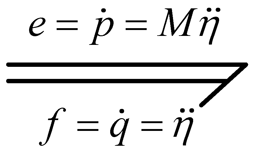
2.1. Modal Vector Bond Graph Concepts

Conventional bond graphs use power and energy variables: flow variables $f$, potential variables $e$, generalized displacements $q$, and generalized momentum $p$. They apply the four variable forms to construct a unified model of the physical system; the bond graph theory was described in detail in Ref. [20]. The conventional power bond can be represented as an n-dimensional modal vector bond form, as shown in Figure 1.

Figure 1. n-dimensional mode vector bond.

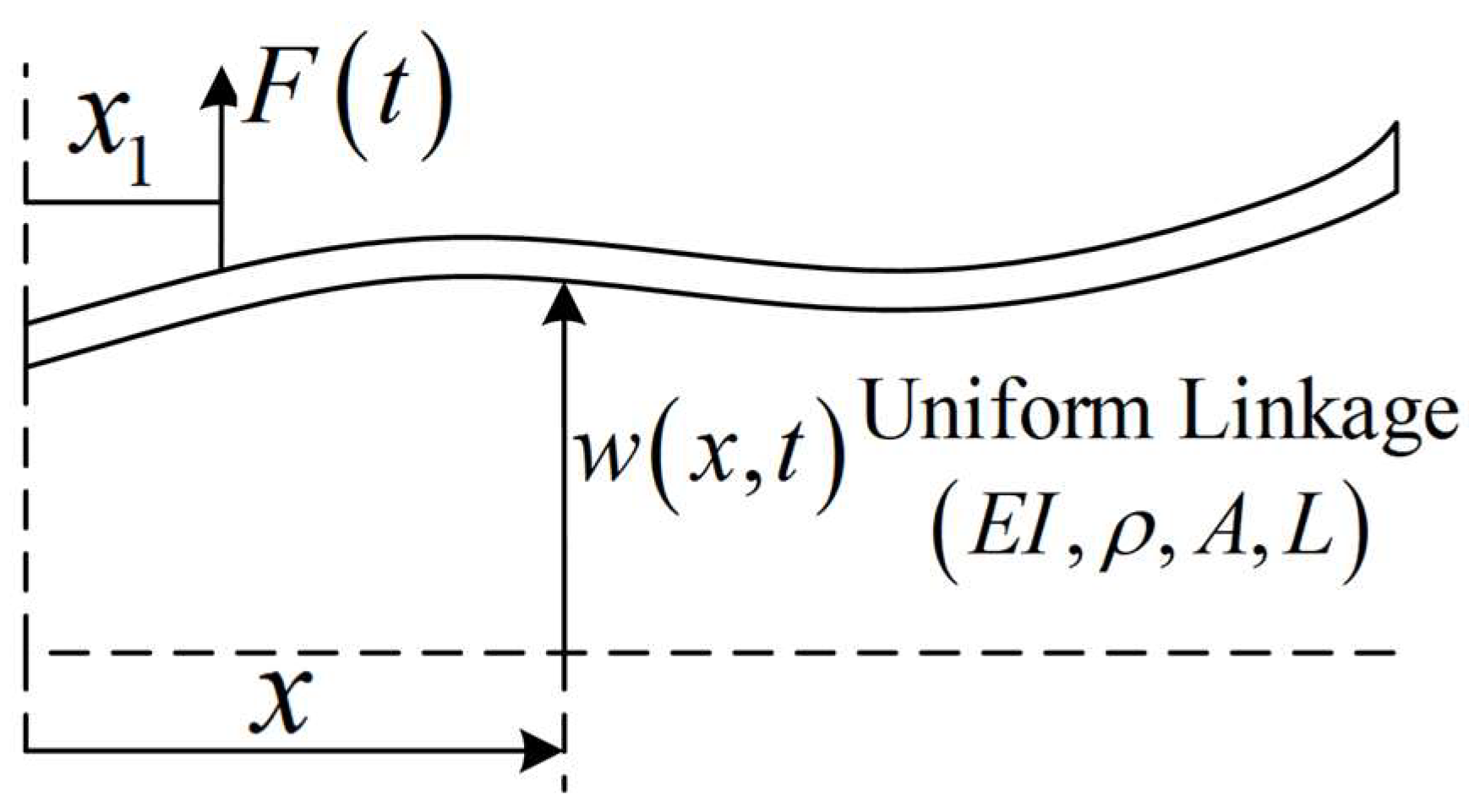
2.2. Flexible Connecting Rod Bond Graph Modeling

Considering the flexibility of the rods, the flexible rods can be regarded as Euler–Bernoulli beams and modeled as bond graphs based on the assumed modal method. The longitudinal vibration of the connecting rod is neglected, and only the bending vibration of the connecting rod is considered. If the connecting rod is subjected to a concentrated force, $F(t)$ at $x=x_1$, as shown in Figure 2.

Figure 2. Uniform flexible linkage subjected to external force $F$.

The concentrated force $F(t)$ can be transformed into a distributed force form $F(t)\delta (x-x_1)$, and then the vibration equation of the flexible rod can be expressed as:

$$EI{\displaystyle \frac{{\partial }^{4}w\left(x,t\right)}{\partial x^4}}+\rho A{\displaystyle \frac{{\partial }^{2}w\left(x,t\right)}{\partial t^2}}=F(t)\delta (x-x_1)$$

(1)

where $w$ is the deflection of the rod, $E$ is the modulus of elasticity of the material, $I$ is the moment of inertia of the cross-section, $\rho$ is the density of the material, and $A$ is the cross-sectional area.

The response of a flexible rod, either forced or unforced, is expressed as a linear combination of the vibration patterns, i.e.,

$$w\left(x,t\right)={\displaystyle \sum _{n=1}^{\infty }{Y}_n(x){\eta }_n(t)}, n=1,2,\cdots$$

(2)

Applying Equation (2) to the vibration Equation (1) by multiplying each term by $Y_m(x)$ and taking the integrals from $x=0$ to $x=L$ for $x$, and then utilizing the orthogonality of the modes, i.e., $Y_n(x)=Y_m(x)$ only when $n=m$ and 0 for the rest of the parts, then the following expression is obtained,

$$({\displaystyle {\int }_0^L\rho A}{Y}_n^{2}dx){\ddot{\eta }}_n+({\displaystyle {\int }_0^L\rho A}{Y}_n^{2}dx){\omega }_n^2{\eta }_n=F(t)Y_n(x_1)$$

(3)

where the modal mass is expressed as

$$m_n={\displaystyle {\int }_0^L\rho A}{Y}_n^{2}dx,n=1,2,\cdots$$

The modal stiffness is expressed as

$$k_n=({\displaystyle {\int }_0^L\rho A}{Y}_n^{2}dx){\omega }_n^2=m_n{\omega }_n^2,n=1,2,\cdots$$

At this point, Equation (3) can be expressed as

$$m_n{\ddot{\eta }}_n+k_n{\eta }_n=F(t)Y_n(x_1),n=1,2,\cdots$$

(4)

In addition, considering the existence of a rigid-body mode, i.e., translational motion of the whole flexible rod and rotational motion around the center of mass, in addition to the transverse vibration of the flexible rod under the action of an external force, it is obtained that

$$m{\ddot{\eta }}_{00}=F(t)$$

(5)

$$J{\ddot{\eta }}_0=F(t)(x_1-{\displaystyle \frac{L}{2}})$$

(6)

where Equation (5) represents the effect of external force on the acceleration of the center of mass of the flexible rod, ${\ddot{\eta }}_{00}$ is the acceleration of the center of mass, and $m$ is the mass of the flexible rod. Equation (6) represents the effect of the moment of the external force on the angular acceleration of the center of mass, and $J$ is the rotational moment of inertia of the flexible rod around the center of mass.

Rewrite Equation (4) in the form of a bond graph energy variable:

$$\dot{\mathit{p}}+\mathit{K}\mathit{q}=F(t)\mathit{Y}(x_1)$$

(7)

where $\mathit{K}=\left[\begin{array}{cccc}{k}_1& & & \\ & k_2& & \\ & & \dots & \\ & & & k_n\end{array}\right]$ is the mode stiffness matrix; the form is a diagonal angular array with diagonal elements for each order of modal stiffness;

$\mathit{Y}(x_1)={\left[\begin{array}{cccc}{Y}_1(x_1)& Y_2(x_1)& \cdots & Y_n(x_1)\end{array}\right]}^T$ is a vector of vibrational mode functions.

According to Equations (5)–(7), the flexible rod modal vector bond graph is established, as shown in Figure 3.

Figure 3. Mode vector bond graph of flexible linkage subjected to external force $F$ at $x=x_1$.

The modulus of the converter -MTF- in Figure 3 is a vector of vibrational functions, representing the system’s conversion from a physical space variable to a modal space variable and its inverse transformation.

If the flexible rod is subjected not only to an external force, but also to an external moment, then the equation of vibration shown in Equation (3) will change to

$$EI{\displaystyle \frac{{\partial }^{4}w\left(x,t\right)}{\partial x^4}}+\rho A{\displaystyle \frac{{\partial }^{2}w\left(x,t\right)}{\partial t^2}}=f(x,t)-{\displaystyle \frac{\partial }{\partial x}}\tau (x,t)$$

(8)

Using the same derivation process, the external moment is fed into the vector bond graph by the corresponding -TF- transformer, but then the modulus of the transformer is the slope of the vibrational mode at the point where the moment is acting, i.e.,

$$\mathit{d}\mathit{Y}={\left[\begin{array}{cccc}d{Y}_1/dx& d{Y}_2/dx& \cdots & d{Y}_3/dx\end{array}\right]}^T.$$

The flexible rod modal vector bond graph model shown in Figure 3 is generalized to represent all flexible structures with typical oscillation characteristics. Due to the different systems, the vibration mode function matrix, modal mass matrix, and modal stiffness matrix will change under different boundary conditions and initial conditions, but the structural form of the vector bond graph remains unchanged, so it is treated as a flexible unit module. When the flexible rod interacts with the external power element or physical system, the external system can be directly connected to the force source Se passport in the Figure, which is introduced into the modal vector bond graph from the 0-junction. At this time, $F(t)$ becomes the internal force, while the unit module of the modal vector bond graph structure form remains unchanged. In addition, in this modular model, the modal response of each order of the flexible rod is included, and the rigid-body motion pattern caused by the external force is included.

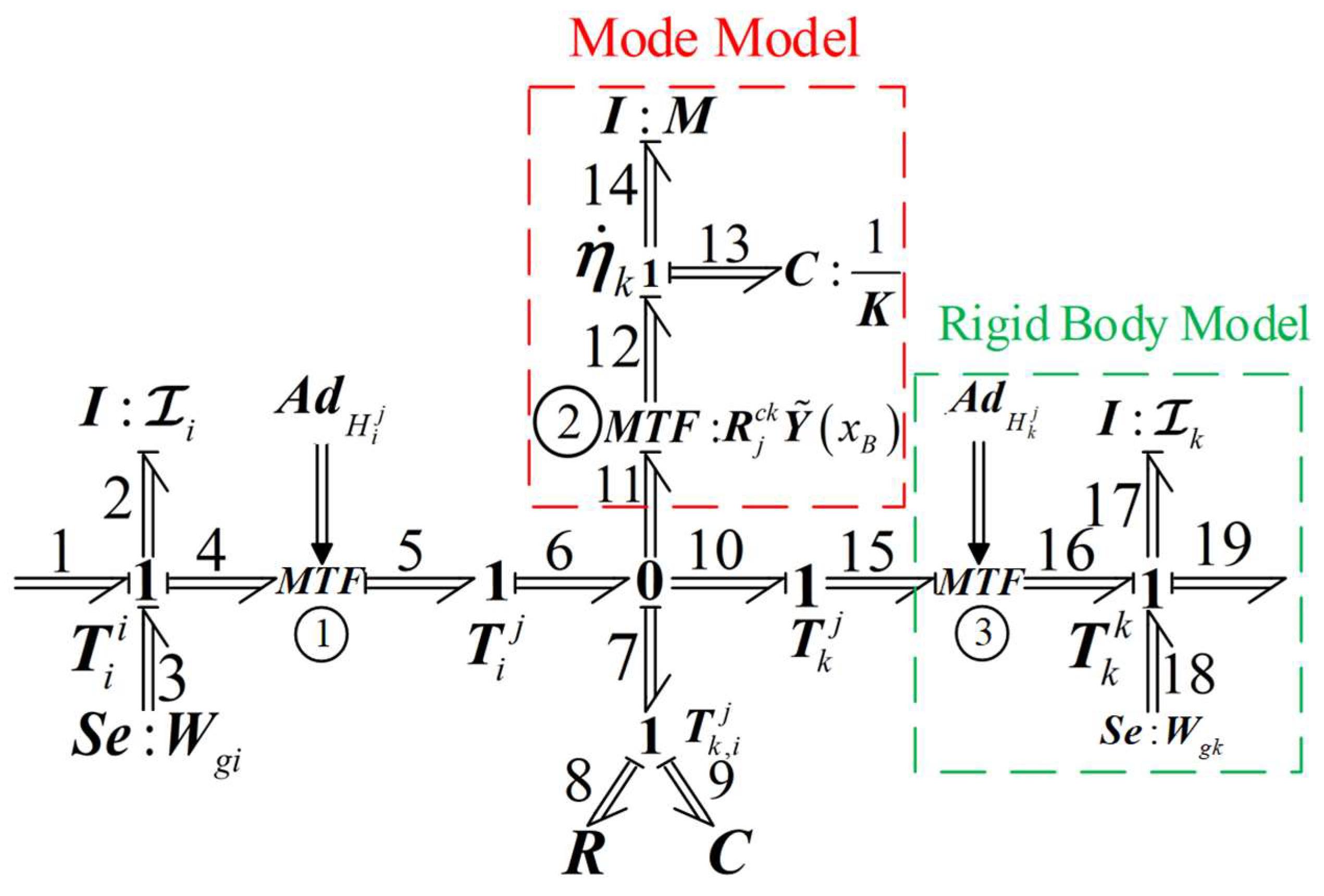
2.3. Hybrid Bond Graph Rigid–Flexible Coupled Rod System

As shown in Figure 4, it is a rod system composed of two connecting rods connected by a revolute joint, assuming that the connecting rod $i$ is a rigid body, and the connecting rod $k$ is an elongated rod of equal cross-section with a length of $L$, which is regarded as a flexible rod. The center of the revolute joint is $B$, the angle of the flexible rod is ${\theta }_j$, $O–xy$ is the inertial coordinate system ${\Psi }_0$, the center of mass of the flexible rod is $k$, and $Ock–XckYck$ is the link coordinate system ${\Psi }_{ck}$.

Figure 4. Rigid–flexible coupling linkage system.

The flexible rod modal vector bond graph unit module model, combined with the rigid body and joint screw bond graph model, is used to construct the rigid–flexible coupled rod system bond graph model, as shown in Figure 5.

Figure 5. Bond graph model of rigid–flexible coupled linkage system.

In the integral causality, the $p$ variable on the energy element $I–$element and the $q$ variable on the $C–$element are chosen as the state variables of the system, and the equation of the state of the system is obtained by deriving according to the rules.

$$\left\{\begin{array}{l}{\dot{p}}_2=e_1-e_3-e_{7}MT{F}_{①}\hfill \\ {\dot{p}}_{14}=e_{7}MT{F}_{②}-{\displaystyle \frac{q_{13}}{c_{13}}}\hfill \\ {\dot{p}}_{17}=e_{7}MT{F}_{③}-e_{18}-e_{19}\hfill \\ {\dot{q}}_{13}={\displaystyle \frac{p_{14}}{I_{14}}}\hfill \\ {\dot{q}}_9={\displaystyle \frac{p_2}{I_2}}MT{F}_{①}-{\displaystyle \frac{p_{14}}{I_{14}}}MT{F}_{②}-{\displaystyle \frac{p_{17}}{I_{17}}}MT{F}_{③}\hfill \end{array}\right.$$

(9)

where one of the outputs of the system is the joint binding,

$$\begin{array}{ll}{e}_7& =e_8+e_9=R_8{f}_8+{\displaystyle \frac{q_9}{C_9}}\\ & =R_8({\displaystyle \frac{p_2}{I_2}}MT{F}_{①}-{\displaystyle \frac{p_{14}}{I_{14}}}MT{F}_{②}-{\displaystyle \frac{p_{17}}{I_{17}}}MT{F}_{③})+{\displaystyle \frac{q_9}{C_9}}\end{array}$$

(10)

Describing the system state Equation (10) using the matrix form, the

$$\dot{\tilde{\mathit{X}}}=\mathit{A}\tilde{\mathit{X}}+\mathit{U}$$

(11)

Among them, $\tilde{\mathit{X}}={\left[\begin{array}{ccc}{\mathcal{I}}_i{\mathit{T}}_i^i& {\mathit{K}}_{kn}{\dot{\mathit{\eta }}}_{kn}& \begin{array}{ccc}{\mathcal{I}}_k{\dot{\mathit{\eta }}}_{k0}& {\mathit{\eta }}_{kn}& {\mathit{q}}_9\end{array}\end{array}\right]}^{\mathrm{T}}$;

$$\begin{gathered} \mathit{A}=\left[\begin{array}{ccccc}-{\displaystyle \frac{R_8}{{\mathcal{I}}_i}}{\left(\mathit{A}{\mathit{d}}_{H_i^j}\right)}^2& {\displaystyle \frac{R_8}{M}}{\mathit{R}}_j^{ck}\tilde{\mathit{Y}}\left(x_B\right)\mathit{A}{\mathit{d}}_{H_i^j}& -{\displaystyle \frac{R_8}{{\mathcal{I}}_k}}\mathit{A}{\mathit{d}}_{H_k^j}\mathit{A}{\mathit{d}}_{H_i^j}& 0& -{\displaystyle \frac{1}{C_9}}\mathit{A}{\mathit{d}}_{H_i^j}\\ {\displaystyle \frac{R_8}{{\mathcal{I}}_i}}\mathit{A}{\mathit{d}}_{H_i^j}{\mathit{R}}_j^{ck}\tilde{\mathit{Y}}\left(x_B\right)& -{\displaystyle \frac{R_8}{M}}{\left[{\mathit{R}}_j^{ck}\tilde{\mathit{Y}}\left(x_B\right)\right]}^2& {\displaystyle \frac{R_8}{{\mathcal{I}}_k}}\mathit{A}{\mathit{d}}_{H_k^j}{\mathit{R}}_j^{ck}\tilde{\mathit{Y}}\left(x_B\right)& -K& {\displaystyle \frac{1}{C_9}}{\mathit{R}}_j^{ck}\tilde{\mathit{Y}}\left(x_B\right)\\ {\displaystyle \frac{R_8}{{\mathcal{I}}_i}}\mathit{A}{\mathit{d}}_{H_i^j}\mathit{A}{\mathit{d}}_{H_k^j}& -{\displaystyle \frac{R_8}{M}}{\mathit{R}}_j^{ck}\tilde{\mathit{Y}}\left(x_B\right)\mathit{A}{\mathit{d}}_{H_k^j}& -{\displaystyle \frac{R_8}{{\mathcal{I}}_k}}{\left(\mathit{A}{\mathit{d}}_{H_k^j}\right)}^2& 0& {\displaystyle \frac{1}{C_9}}\mathit{A}{\mathit{d}}_{H_k^j}\\ 0& {\displaystyle \frac{1}{M}}& 0& 0& 0\\ {\displaystyle \frac{R_8}{{\mathcal{I}}_i}}\mathit{A}{\mathit{d}}_{H_i^j}& -{\displaystyle \frac{R_8}{M}}{\mathit{R}}_j^{ck}\tilde{\mathit{Y}}\left(x_B\right)& -{\displaystyle \frac{R_8}{{\mathcal{I}}_k}}\mathit{A}{\mathit{d}}_{H_k^j}& 0& 0\end{array}\right] \\ \mathit{U}={\left[\begin{array}{ccccc}{e}_1-W_{gi}& 0& -W_{gk}-e_{19}& 0& 0\end{array}\right]}^{\mathrm{T}}. \end{gathered}$$

For the free response, assume $\mathit{U}=0$, and express the state variable as an exponential function, i.e., the

$$\tilde{\mathit{X}}=\mathit{\Psi }{e}^{st}$$

(12)

Then, Equation (11) becomes

$$s\mathit{\Psi }{e}^{st}=A\mathit{\Psi }{e}^{st}$$

(13)

Introducing the unitary matrix $s\mathit{I}\mathit{\Psi }{e}^{st}=\mathit{A}\mathit{\Psi }{e}^{st}$, further synthesized

$$\left(s\mathit{I}-\mathit{A}\right)\mathit{\Psi }{e}^{st}=0$$

(14)

In order for Equation (14) to hold and obtain a helpful solution, then the following conditions need to be satisfied:

$$\left|s\mathit{I}-\mathit{A}\right|=0$$

(15)

Since $\mathit{A}$ is not a symmetric matrix, according to the complex modal theory, the eigenvalues satisfying the above equation are solved to obtain the intrinsic frequency of the system.

In the bond graph of the rigid–flexible coupled rod system shown in Figure 5, the flow and potential variables on any bond can be used as the system’s output. The system equations are solved in the form of state variables, and then the output equations are derived to correlate the expected output variables with the state variables as shown in Equation (10), which, according to the solution of the equations, makes the expected output of the system observable. The response of the output point can be observed in real-time using automated computer simulation by introducing a potential or current source of size 0 through a 0-junction or 1-junction at the location where it is desired to be observed or measured. For example, to observe the output at the contact point $Ei$ at the position of the flexible rod $x=x_1$, we connect the bond graph shown in Figure 6 to the 1-junction of the modal bond graph of Figure 5 and use computer-automated simulation to obtain the response here.

Figure 6. Output at position $x=x_1$ of the flexible link.

Output the velocity at position $x_1$, i.e., the flow equation at 0-junction,

$$f={\displaystyle \sum _{n=1}^{\infty }{Y}_n(x_1)}{\dot{\eta }}_n$$

(16)

Observing Equation (16), which is the actual Equation (1) taking the partial derivative of ${\displaystyle \frac{\partial w}{\partial t}}(x_1,t)$ for time $t$, which is the output of the velocity at $x=x_1$, verifies the reasonableness of the bond graph.

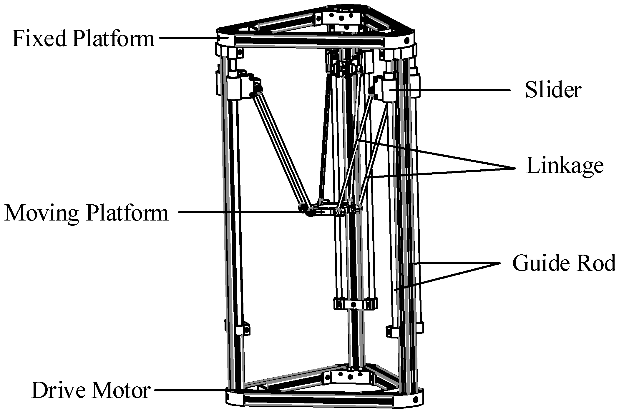
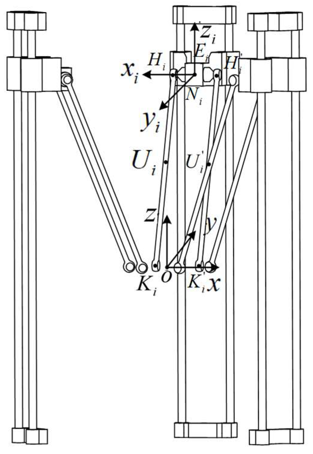
3. Modeling of Spatial Delta-Type Robot Dynamics Considering Linkage Flexibility

3.1. Introduction to the Organization

The Delta-type parallel robot consists of a mechanical body subsystem and a servo-driven control subsystem, the prototype of which is shown in Figure 7 and the structure of which is shown in Figure 8. Its three branched chains are distributed according to 120°, and all of them are composed of guide rods, sliders, connecting rods, and a closed-loop parallelogram mechanism. Considering the lightweight design of the robot linkage, which leads to an increase in its flexibility and a decrease in its intrinsic frequency, its dynamics model is constructed using a modal vector bond graph.

Figure 7. Delta-type rigid–flexible coupling parallel robot.

Figure 8. Mechanism structure of Delta-type rigid–flexible coupling parallel robot.

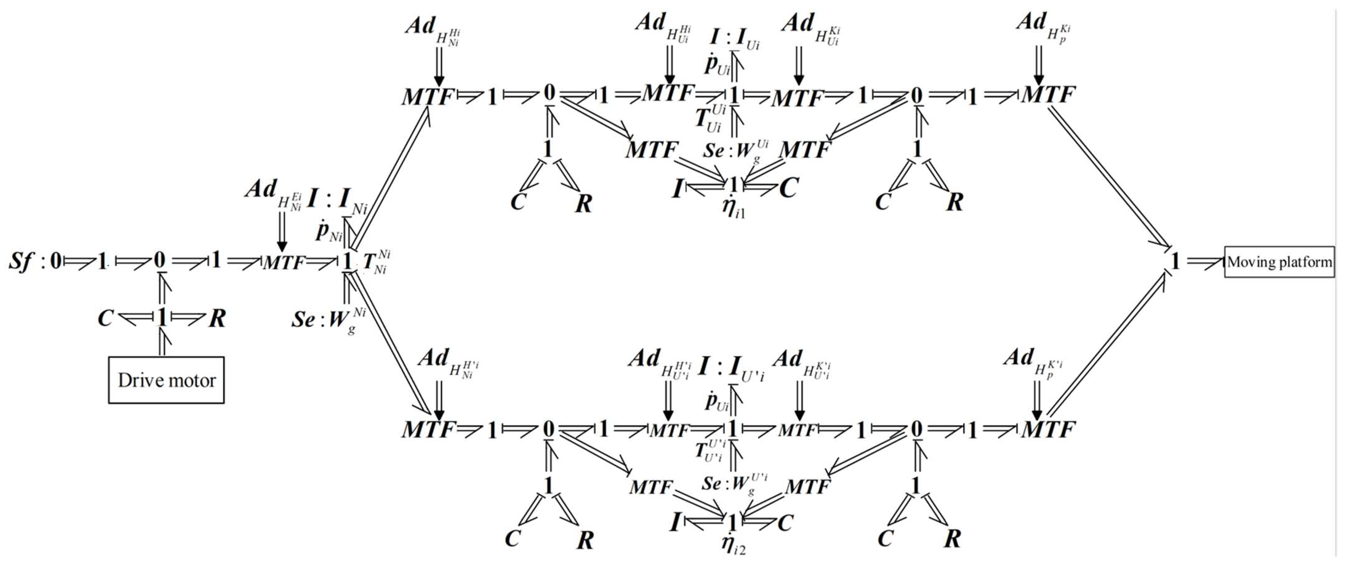
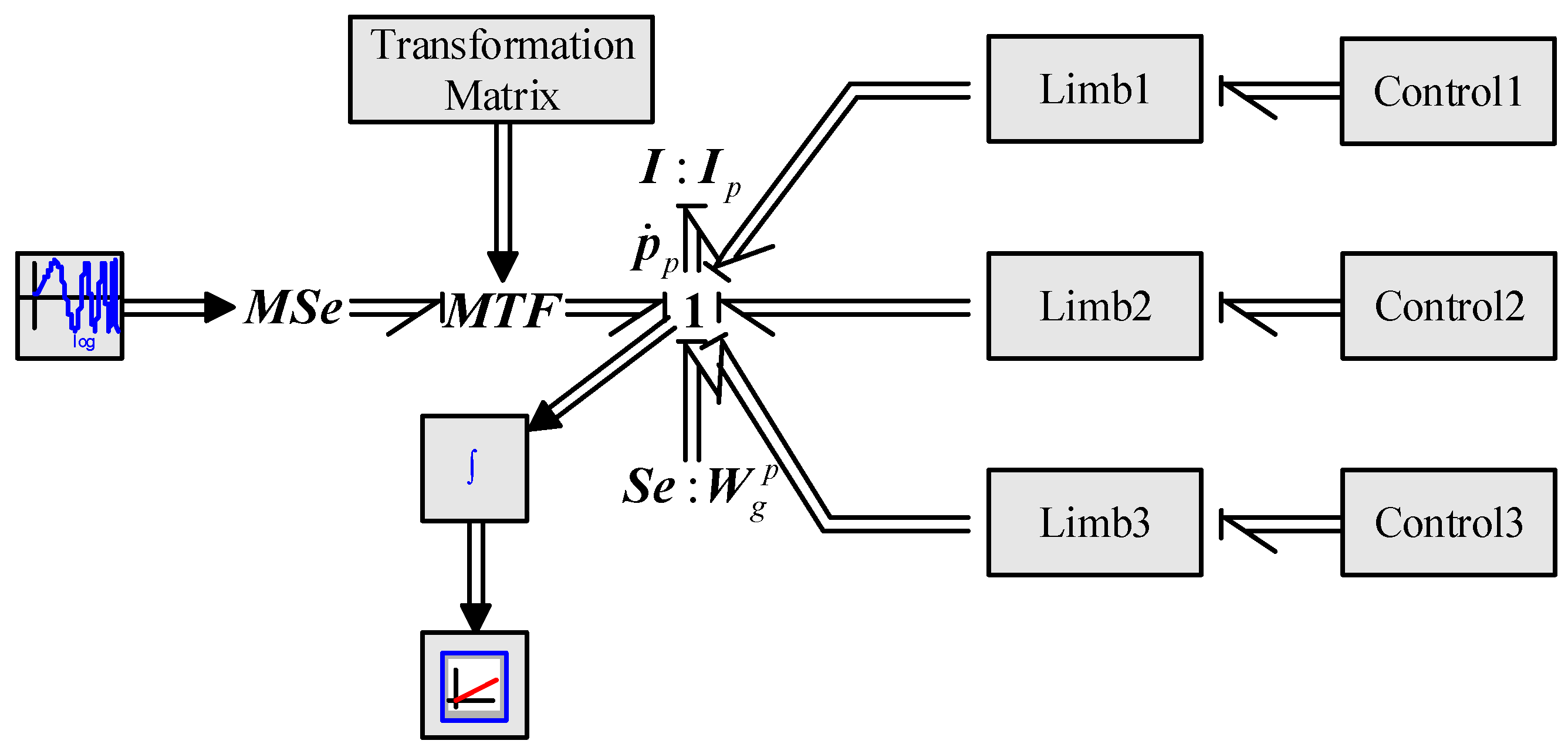
3.2. Rigid–Flexible Coupling Bond Graph Model of Parallel Mechanism

Since the structure of each branch of this robot mechanism is the same, one of the branches is selected for analysis, and the coordinate system, as in Figure 9, is established. The inertial coordinate system ${\Psi }_o$ ($o–xyz$) is established with the center of the motion platform as the origin, the centers of mass of the slider and the two connecting rods $N_i$, $U_i$, and $U_i^{\prime }$, and the constructed center-of-mass coordinate system ${\Psi }_{Ni}$, ${\Psi }_{Ui}$, and ${\Psi }_{U_i^{\prime }}$ ($i=1,2,3$) are parallel to the inertial coordinate system ${\Psi }_o$. The coordinate origins of the coordinate systems ${\Psi }_{Ei}$, ${\Psi }_{Hi}$, ${\Psi }_{H_i^{\prime }}$, ${\Psi }_{Ki}$, and ${\Psi }_{K_i^{\prime }}$ are the contact points of the kinematic joints $E_i$ and the centers of rotation of the spherical joints $H_i$, $H_i^{\prime }$, $K_i$, and $K_i^{\prime }$, respectively, and the coordinate systems are parallel to the branched-chain coordinate system ${\Psi }_i$. The direction of the $z_i$ axis of the branched coordinate system ${\Psi }_i$ is along the up and down sliding direction, and the direction cosine of the $y_i$ axis concerning the inertial coordinate system ${\Psi }_o$ can be expressed as follows

$$\begin{array}{l}{\mathit{y}}_1={\left[\begin{array}{ccc}0& -1& 0\end{array}\right]}^{\mathrm{T}},{\mathit{y}}_2={\left[\begin{array}{ccc}-\sin 60°& \cos 60°& 0\end{array}\right]}^{\mathrm{T}},\\ {\mathit{y}}_3={\left[\begin{array}{ccc}\sin 60°& \cos 60°& 0\end{array}\right]}^{\mathrm{T}},\end{array}$$

Figure 9. Branch chain structure graph.

$x_i$ axes perpendicular to the plane formed by the $y_i$ and $z_i$ axes, that is, ${\mathit{x}}_i={\mathit{y}}_i\times {\mathit{z}}_i$.

Considering the linkage flexibility, the bond graph model of the Delta-type rigid–flexible coupled parallel robot strut chain is established by combining the modal vector bond graph and screw bond graph in Figure 10.

Figure 10. Bond graph of branch chain.

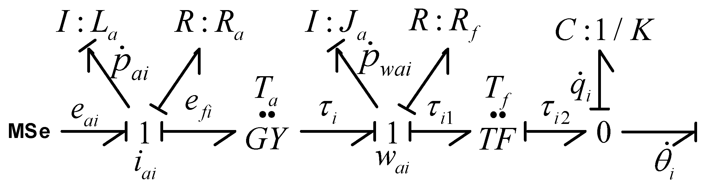
3.3. Constructing a Multi-Energy Domain Rigid–Flexible Coupling Dynamics Model for Robotic Systems

The servomotor provides the drive for the parallel robot, and the bond graph model of the servomotor and reducer is shown in Figure 11. The potential $p$ and current $q$ are chosen as state variables to obtain the state equation of the drive system as

$$\left\{\begin{array}{l}{\stackrel{·}{p}}_{ai}=e_{ai}-T_a{w}_{ai}-R_a{i}_{ai}\hfill \\ {\stackrel{·}{p}}_{wai}=T_a{i}_{ai}-T_f{\displaystyle \frac{q_i}{K}}-R_f\hfill \\ {\stackrel{·}{q}}_i=T_f{w}_{ai}-{\stackrel{·}{\theta }}_i\hfill \end{array}\right.$$

(17)

where $L_a$ and $R_a$ are the inductance and resistance of the armature, respectively, $J_a$ is the rotational inertia of the motor rotor, $T_a$ is the electromagnetic torque constant of the motor, $R_f$ is the equivalent frictional torque of the motor, $T_f$ is the reduction ratio of the gearbox, $K$ is the reduction ratio of the gearbox, $w_{ai}$ is the angular velocity, ${\stackrel{·}{p}}_{ai}$ is the state variable, ${\stackrel{·}{q}}_i$ is the flow variable, and ${\stackrel{·}{\theta }}_i$ is the angular variable.

Figure 11. Bond graph of servo motor and reducer.

Combining the screw bond graph of the mechanical system with the bond graph of the servo system, the global bond graph of one branch chain of the Delta-type rigid–flexible coupled parallel robot can be constructed, as shown in Figure 12. Then, we connect the three branches to the moving platform to obtain a global bond graph of the complete parallel robot, as shown in Figure 13.

Figure 12. Global bond graph of branch chain.

Figure 13. Global bond graph.

3.4. Arithmetic Examples

The robot structure and electrical control parameters are selected, as shown in Table 1 and Table 2. The global bond graph model of the robot is established in the bond graph modeling software 20-sim, based on which the robot system is analyzed [21].

Table 1. Structural parameters of the Delta-type parallel robot.

Parameters	Value
Radius of fixed platform (R/m)	0.233
Length of flexible linkage (L/m)	0.213
Radius of moving platform (r/m)	0.073
Mass of slider ($m_{Ni}$/kg)	0.397
Mass of flexible linkage ($m_{Ui}$/kg)	0.032
Mass of moving platform ($m_P$/kg)	0.195
Young’s modulus of flexible linkage (E/(pa))	2 × 1011
Density of flexible linkage (ρ/(kg/m3))	7.85 × 103

Table 2. Parameters of servo motor and reducer.

Parameters	Value
Winding inductance (H)	1.58 × 10−3
Operating voltage (V)	200
Rotor inertia of motor (kg·m2)	3.12 × 10−4
Winding resistance (Ω)	0.32
Electromagnetic torque constant (N·m/A)	0.34
Equivalent friction torque of motor (N·m)	0.003
Reduction ratio of reducer	0.025
Torque stiffness of reducer (N·m/arcmin)	1.8

4. Simulation-Based Vibration Analysis

Since the multi-energy domain flexible parallel robotic system is a complex system coupled with a control and mechanical subsystem, both the control and mechanical subsystem may cause system vibration. According to these two vibration sources, the vibration analysis of different vibration forms is discussed in the frequency domain.

The servomotor in the control subsystem provides the driving force to drive the mechanical subsystem and receives the actual position/velocity feedback from the mechanical subsystem. Therefore, for the vibration analysis of the control subsystem, the coupling effect of the mechanical subsystem should also be considered. The velocity loop is an important part of the servo motor control system, and its control performance is an important index for evaluating the overall system performance. Without considering the mechanical subsystem, the frequency domain toolbox of 20-sim software can be used to get the closed-loop of different speed loop controller parameters.

Based on the global bond graph, the corresponding state equations for this system are derived:

$$\left\{\begin{array}{l}{\dot{\mathit{p}}}_{Ni}=\mathit{A}{\mathit{d}}_{H_{Ni}^{Ei}}^T{\mathit{e}}_{Ei}+{\mathit{W}}_g^{Ni}-\mathit{A}{\mathit{d}}_{H_{Ni}^{Hi}}^T{\mathit{e}}_{Hi}-\mathit{A}{\mathit{d}}_{H_{Ni}^{H^{\prime }i}}^T{\mathit{e}}_{H^{\prime }i}\hfill \\ {\dot{\mathit{p}}}_{Ui}=\mathit{A}{\mathit{d}}_{H_{Ui}^{Hi}}^T{\mathit{e}}_{Hi}+{\mathit{W}}_g^{Ui}-\mathit{A}{\mathit{d}}_{H_{Ui}^{Ki}}^T{\mathit{e}}_{Ki}\hfill \\ {\dot{\mathit{p}}}_{U^{\prime }i}=\mathit{A}{\mathit{d}}_{H_{U^{\prime }i}^{H^{\prime }i}}^T{\mathit{e}}_{H^{\prime }i}+{\mathit{W}}_g^{U^{\prime }i}-\mathit{A}{\mathit{d}}_{H_{U^{\prime }i}^{K^{\prime }i}}^T{\mathit{e}}_{K^{\prime }i}\hfill \\ {\dot{\mathit{p}}}_{\mathit{p}}={\displaystyle \sum _{i=1}^3\mathit{A}{\mathit{d}}_{H_{\mathit{p}}^{Ki}}^T{\mathit{e}}_{Ki}}+{\displaystyle \sum _{i=1}^3\mathit{A}{\mathit{d}}_{H_{\mathit{p}}^{K^{\prime }i}}^T{\mathit{e}}_{K^{\prime }i}}+{\mathit{W}}_g^{\mathit{p}}+\mathit{A}{\mathit{d}}_{H_{\mathit{p}}^o}^T{\mathit{e}}_o\hfill \\ \begin{array}{l}{\dot{\mathit{p}}}_{Mi1}={\mathit{e}}_{Hi}\mathit{M}\mathit{T}{\mathit{F}}_{ci1,xHi}+{\mathit{e}}_{Ki}\mathit{M}\mathit{T}{\mathit{F}}_{ci1,xKi}-{\displaystyle \frac{{\mathit{q}}_{ci1}}{{\mathit{c}}_{i1}}}\\ {\dot{\mathit{p}}}_{Mi2}={\mathit{e}}_{H^{\prime }i}\mathit{M}\mathit{T}{\mathit{F}}_{ci2,x{H}^{\prime }i}+{\mathit{e}}_{K^{\prime }i}\mathit{M}\mathit{T}{\mathit{F}}_{ci2,x{K}^{\prime }i}-{\displaystyle \frac{{\mathit{q}}_{\mathit{c}i2}}{{\mathit{c}}_{i2}}}\\ {\dot{\mathit{q}}}_{ci1}={\displaystyle \frac{{\mathit{p}}_{Mi1}}{{\mathit{I}}_{Mi1}}}\\ {\dot{\mathit{q}}}_{ci2}={\displaystyle \frac{{\mathit{p}}_{Mi2}}{{\mathit{I}}_{Mi2}}}\\ {\dot{\mathit{q}}}_{cEi}={\dot{\mathit{\theta }}}_i\mathit{M}\mathit{T}\mathit{F}={\displaystyle \frac{{\mathit{p}}_{Ni}}{{\mathit{I}}_{Ni}}}\mathit{A}{\mathit{d}}_{H_{Ni}^{Ei}}\\ {\dot{\mathit{q}}}_{cHi}={\displaystyle \frac{{\mathit{p}}_{Ni}}{{\mathit{I}}_{Ni}}}\mathit{A}{\mathit{d}}_{H_{Ni}^{Hi}}-{\displaystyle \frac{{\mathit{p}}_{Ui}}{{\mathit{I}}_{Ui}}}\mathit{A}{\mathit{d}}_{H_{Ui}^{Hi}}-{\displaystyle \frac{{\mathit{p}}_{Mi1}}{{\mathit{I}}_{Mi1}}}\mathit{M}\mathit{T}{\mathit{F}}_{ci1,xHi}\\ {\dot{\mathit{q}}}_{cKi}={\displaystyle \frac{{\mathit{p}}_{Ui}}{{\mathit{I}}_{Ui}}}\mathit{A}{\mathit{d}}_{H_{Ui}^{Ki}}-{\displaystyle \frac{{\mathit{p}}_{\mathit{p}}}{{\mathit{I}}_{\mathit{p}}}}\mathit{A}{\mathit{d}}_{H_{\mathit{p}}^{Ki}}-{\displaystyle \frac{{\mathit{p}}_{Mi1}}{{\mathit{I}}_{Mi1}}}\mathit{M}\mathit{T}{\mathit{F}}_{ci1,xKi}\\ {\dot{\mathit{q}}}_{c{H}^{\prime }i}={\displaystyle \frac{{\mathit{p}}_{Ni}}{{\mathit{I}}_{Ni}}}\mathit{A}{\mathit{d}}_{H_{Ni}^{H^{\prime }i}}-{\displaystyle \frac{{\mathit{p}}_{U^{\prime }i}}{{\mathit{I}}_{U^{\prime }i}}}\mathit{A}{\mathit{d}}_{H_{U^{\prime }i}^{H^{\prime }i}}-{\displaystyle \frac{{\mathit{p}}_{Mi2}}{{\mathit{I}}_{Mi2}}}\mathit{M}\mathit{T}{\mathit{F}}_{ci2,x{H}^{\prime }i}\\ {\dot{\mathit{q}}}_{c{K}^{\prime }i}={\displaystyle \frac{{\mathit{p}}_{U^{\prime }i}}{{\mathit{I}}_{U^{\prime }i}}}\mathit{A}{\mathit{d}}_{H_{U^{\prime }i}^{K^{\prime }i}}-{\displaystyle \frac{{\mathit{p}}_{\mathit{p}}}{{\mathit{I}}_{\mathit{p}}}}\mathit{A}{\mathit{d}}_{H_{\mathit{p}}^{K^{\prime }i}}-{\displaystyle \frac{{\mathit{p}}_{Mi2}}{{\mathit{I}}_{Mi2}}}\mathit{M}\mathit{T}{\mathit{F}}_{ci2,x{K}^{\prime }i}\end{array}\hfill \end{array}\right.$$

(18)

Frequency response is shown in Figure 14. The data in parentheses in the Figure are the scaling factor $k_{pv}$ and the integration time constant $k_{iv}$. From Figure 14, it can be seen that the higher the controller parameters, the greater the bandwidth of the control subsystem and the faster the response of the system. However, the increase in bandwidth also increases the shear frequency of the system, the phase stability margin of the system decreases, and in the middle-frequency band, the phase lag is less than the lower bandwidth at the same frequency. When considering the mechanical subsystem, the response curves of servo motors with different velocity loop controller parameters to unit stepping signals are simulated in 20-sim, as shown in Figure 15. The power spectral density (PSD) analysis of the signals in Figure 15 yields Figure 16. Based on the response speeds of different velocity loop controller parameters to the stepping signals in Figure 15, it can be shown that system A responds the fastest and performs the best in multiple datasets. Corresponding to Figure 16, it can also be seen that the resonance amplitude of the optimal parameters is lower in the frequency domain analysis.

Figure 14. Closed-loop frequency response of speed loop.

Figure 15. Step response of speed loop.

Figure 16. Power spectral density of velocity loop step response.

The position loop in the control system is mainly used to ensure the system’s static positional accuracy and dynamic tracking performance so that the servo motor system can run smoothly and perform at a high dynamic level. Usually, a P controller is used to keep the overshoot and steady-state error as small as possible. The closed-loop frequency response of different position loop controller parameters without considering the mechanical subsystem can be obtained through the frequency domain toolbox of 20-sim software, as shown in Figure 17. From Figure 17, it can be seen that the higher the parameters of the position controller, the larger the bandwidth of the control subsystem and the faster the response of the system. When considering the mechanical subsystem, the response curves of servo motors with different position loop parameters to the unit stepping signals are simulated in 20-sim, as shown in Figure 18. The power spectral density (PSD) analysis of the signals in Figure 18 yields Figure 19. Based on the response speeds of the different position loop controller parameters to the stepping signals in Figure 18, it can be concluded that the system $k_{pp}=10,000$ has the fastest response and the best performance among the several sets of data. The resonance amplitude is the lowest in the frequency domain analysis in Figure 19.

Figure 17. Closed-loop frequency response of position loop.

Figure 18. Step response of position loop.

Figure 19. Power spectral density of position loop step response.

For mechanical subsystems, load capacity is an important performance metric for flexible parallel robots. The excitation force of the load can be simulated by applying a sinusoidal swept frequency signal with an amplitude of 1 V to the moving platform, and the displacement of the end of the moving platform is used as the output signal. Frequency response analysis was performed using the frequency domain toolbox of 20-sim software to evaluate the FRF value of the moving platform.

The swept excitation signal was utilized to identify the frequency response in the z-direction and obtain the intrinsic frequency in that direction. Figure 20 shows the sinusoidal swept frequency signal with an amplitude of 1 V. Figure 21 shows the frequency response function curve of the moving platform in the z-direction. From Figure 21, it can be seen that the first-order and second-order intrinsic frequencies of the mechanical subsystem are 234.7 Hz and 531.3 Hz, respectively.

Figure 20. Sweep signal.

Figure 21. Frequency response of the moving platform in the z-direction.

The computer model of the Delta-type rigid–flexible coupled parallel robot was established and imported into the ADAMS software to analyze the intrinsic frequency, as shown in Figure 22. Through the vibration module of ADAMS, the first-order intrinsic frequency and the second-order intrinsic frequency of the Delta-type rigid–flexible coupled parallel robot can be obtained, which are 229.09 Hz and 524.80 Hz, respectively. Therefore, it can be concluded that the relative deviations of the simulated frequency of the 20-sim and the simulated frequency of the ADAMS are 2.45% and 1.24%, respectively, which verifies the reasonableness of the bond graph model.

Figure 22. ADAMS simulation model of Delta-type rigid–flexible coupled parallel robot.

When the coupling effects of the control and mechanical subsystems are considered simultaneously, the power spectral density curves of the frequency response function of the moving platform can be observed with different speed loop controller parameter settings, as shown in Figure 23. It can be seen that the amplitudes of both the first resonance peak and the second resonance peak decrease with the increase of the scaling factor $k_{pv}$ and the integration time constant $k_{iv}$, which indicates that lower speed controller parameters are more likely to cause the coupled vibration of the control subsystem and the mechanical subsystem, which results in larger resonance amplitudes.

Figure 23. Power spectral density of the moving platform frequency response function (different speed loop control parameters). (a) $\left(k_{pv},k_{iv}\right)=\left(2,0.02\right)$; (b) $\left(k_{pv},k_{iv}\right)=\left(4,0.04\right)$; (c) $\left(k_{pv},k_{iv}\right)=\left(6,0.06\right)$.

In addition, by setting different position loop controller parameters, the power spectral density curve of the frequency response function of the moving platform can be observed, as shown in Figure 24. It can be seen that the amplitude of the first resonance peak increases with the increase of the scaling factor $k_{pp}$, which indicates that the larger the position controller parameter is, the easier it is to cause the coupled vibration of the control subsystem and the mechanical subsystem.

Figure 24. Power spectral density of moving platform frequency response function (different position loop control parameters). (a) $k_{pp}=6000$; (b) $k_{pp}=8000$; (c) $k_{pp}=\mathrm{10,000}$.

5. Conclusions

This paper presents the modal vector bond graph and the screw bond graph proposed to model the elastic deformation of the flexible body and the rigid body modes contained in its force movement process; a modular model of a flexible rod unit is constructed, which has generality and a simple structural form. It can directly interact with the external physical system or power element based on which the rigid–flexible coupled rod system is modeled, and the dynamic characteristics of the rigid–flexible coupled system can be analyzed based on the equation of state. The key contributions and findings are summarized as follows:

(1)

In this study, the expression form and graphical modeling of the unified essential elements of the bond graph are used to establish a system model containing multiple energy domains and rigid–flexible coupling. The structural form of the model corresponds to the physical structure. A computer simulation model is generated; in addition, there is a unified mathematical description between the equations of state of various energy domains, and it is easy to establish a functional relationship between the desired outputs of the system and the equations of state so that the outputs are observable.

(2)

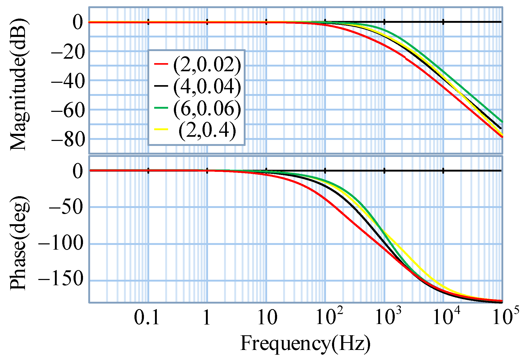
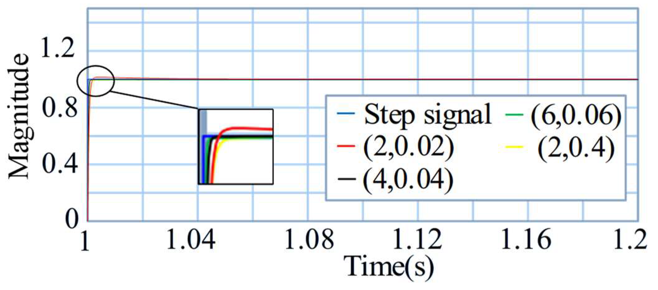
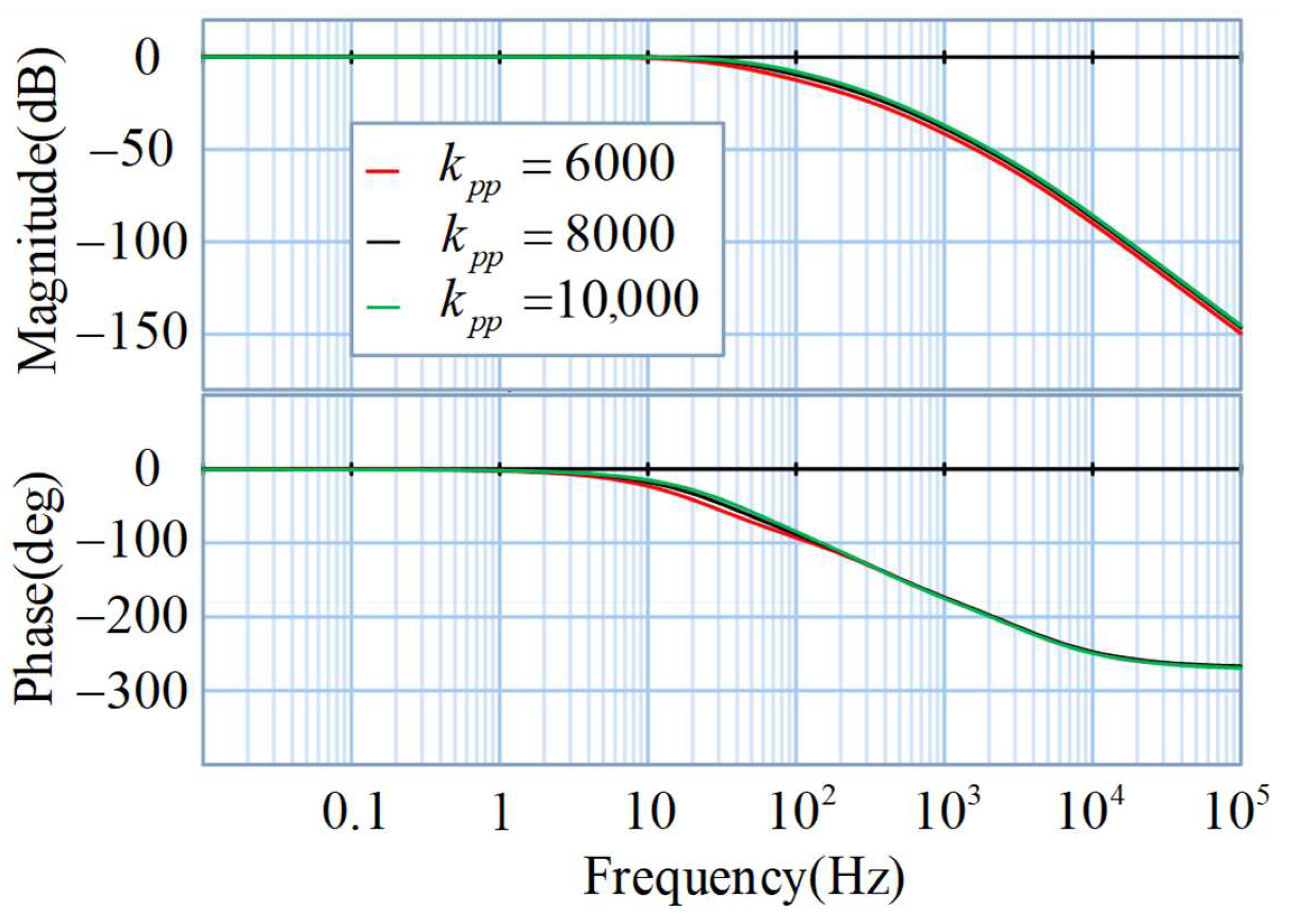
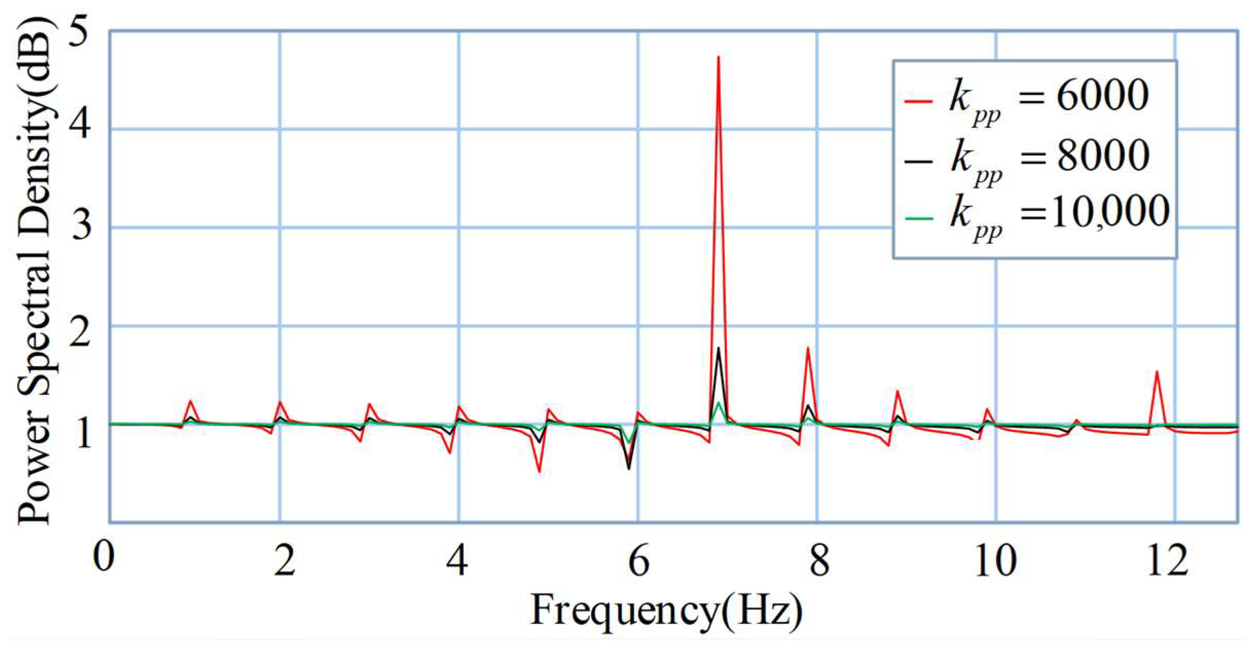
Simulation analysis was carried out based on the model. From the simulation results, the model’s first-order and second-order intrinsic frequencies are 229.09 Hz and 524.80 Hz, respectively, and the mechanical subsystems’ first-order and second-order intrinsic frequencies are 234.7 Hz and 531.3 Hz, respectively. Therefore, it can be concluded that the relative deviations of the simulated frequency of the 20-sim simulation from the simulated frequency of ADAMS are, respectively, 2.45% and 1.24%, which verifies the reasonableness of the bond graph models and derives the influence of different control system parameters on the system, laying a foundation for the subsequent control system design.

References

1. Qin, B.; Zhang, L.; Zhang, Y.; Sang, D. Joint simulation analysis of rigid flexible coupling of Delta parallel robot. Mod. Mach. 2019, 3, 1–4. [Google Scholar] [CrossRef]
2. Sheng, L.; Li, W.; Wang, Y.; Yang, X.; Fan, M. Rigid-flexible coupling dynamic model of a flexible planar parallel robot for modal characteristics research. Adv. Mech. Eng. 2019, 11, 1687814018823469. [Google Scholar] [CrossRef]
3. Shang, L.; Huang, X.; Huang, Y.; Zhang, T. Nonlinear Hybrid Control of Rigid Flexible Coupling Delta Robot Based on Singular Perturbation. J. Mech. Eng. 2024, 60, 124–133. [Google Scholar]
4. Shang, D.; Huang, Y.; Huang, X.; Pan, Z. Research on Rigid-flexible Coupling Dynamics of Delta Parallel Robot Based on Kane Equation Perturbation. J. Mech. Eng. 2024, 60, 95–106. [Google Scholar]
5. Zhang, Q.; Zhao, X.; Liu, L.; Dai, T. Dynamic Modeling and Vibration Simulation of Spatial Flexible Closed-chain Robot. Trans. Chin. Soc. Agric. Mach. 2021, 52, 401–409. [Google Scholar]
6. Chen, P.; Zhang, H. Optimal Control of Motion Stability of Parallel Robot. Comput. Simul. 2018, 35, 291–295. [Google Scholar]
7. Liu, L.; Zhao, X.; Zhou, H.; Wang, J. Dynamic Solution for Spatial Rigid-flexible Parallel Robot. Trans. Chin. Soc. Agric. Mach. 2018, 49, 376–384. [Google Scholar]
8. Kang, B.; Mills, J.K. Vibration control of a planar parallel manipulator using piezoelectric actuators. J. Intell. Robot. Syst. 2005, 42, 51–70. [Google Scholar] [CrossRef]
9. Kang, B.; Mills, J.K. Dynamic modeling of structurally-flexible planar parallel manipulator. Robotica 2002, 20, 329–339. [Google Scholar] [CrossRef]
10. Briot, S.; Khalil, W. Recursive and symbolic calculation of the elastodynamic model of flexible parallel robots. Int. J. Robot. Res. 2013, 33, 469–483. [Google Scholar] [CrossRef]
11. Sun, T.; Song, Y.-M.; Yan, K. Kineto-static analysis of a novel high-speed parallel manipulator with rigid-flexible coupled links. J. Cent. South Univ. 2011, 18, 593–599. [Google Scholar] [CrossRef]
12. Yu, Y.-Q.; Du, Z.-C.; Yang, J.-X.; Li, Y. An Experimental Study on the Dynamics of a 3-RRR Flexible Parallel Robot. IEEE Trans. Robot. 2011, 27, 992–997. [Google Scholar] [CrossRef]
13. Yu, Y.; Xu, Q. Dynamic Modeling and Characteristic Analysis of Compliant Mechanisms Based on PR Pseudo-rigid-body Model. Trans. Chin. Soc. Agric. Mach. 2013, 44, 225–229. [Google Scholar]
14. Sun, Z.H.; Cheng, M.L. Mechanical Characteristics Analysis on Flexible Mattress in Downstream Sinking Based on Lumped Mass Method. Appl. Mech. Mater. 2014, 580–583, 1910–1917. [Google Scholar] [CrossRef]
15. Zhang, Q.; Zhang, X. Dynamic analysis of planar 3-RRR flexible parallel robots under uniform temperature change. J. Vib. Control 2013, 21, 81–104. [Google Scholar] [CrossRef]
16. Zhang, Q.; Zhang, X. Dynamic modelping and analysis of planar 3-RRR flexible parallel robots. J. Vib. Eng. 2013, 26, 239–245. [Google Scholar] [CrossRef]
17. Karnopp, D.C.; Margolis, D.L.; Rosenberg, R.C. System Dynamics: Modeling and Simulation of Mechatronic Systems; John Wiley & Sons: Hoboken, NJ, USA, 2006. [Google Scholar]
18. Yazman, M.A.; Servettaz, G.; Maschke, B. Bond-Graph Modelling of Flexible Robotic Manipulators. IFAC Proc. Vol. 1989, 22, 327–332. [Google Scholar] [CrossRef]
19. Damić, V. Modelling flexible body systems: A bond graph component model approach. Math. Comput. Model. Dyn. Syst. 2006, 12, 175–187. [Google Scholar] [CrossRef]
20. Lynch, S. Dynamical Systems with Applications Using Mathematica; Springer: Berlin/Heidelberg, Germany, 2007. [Google Scholar]
21. Chen, Y.; Chen, X.; Guo, F.; Meng, C.; Zhang, C.; Chen, Y. Dynamic full solution modeling of HDPE film welding robot thermal-mechanical-electric coupled energy domain system. J. Ration Shock 2022, 41, 60–68. [Google Scholar] [CrossRef]