Improving Classification Performance by Addressing Dataset Imbalance: A Case Study for Pest Management

Abstract

Imbalanced data are a non-trivial problem in deep learning. The high variability in the number of samples composing each category might force learning procedures to become biased towards classes with major cardinality and disregard classes with low instances. To overcome such limitations, common strategies involve data balancing using resampling techniques. The cardinality of overnumbered categories is often lowered by sample deletion, thus reducing the data space where the model can learn from. This paper introduces a new approach based on data balancing without sample deletion, allowing for biasing reduction in instance localization and classification tasks. The method is a multi-stage pipeline starting with data cleaning and data filtering steps and ending with the actual data balancing process, during which overnumbered samples are not deleted but divided into multiple sub-classes. In this way, the model can learn from balanced data distribution in which some classes have a high correlation factor. To evaluate the effectiveness of the method in real-life scenarios, a case study in the field of precision agriculture has been developed, motivated by the fact that the publicly available datasets for pest classification often reflect the real-world imbalanced distribution of pests, making the task challenging. Two models for the localization and recognition of pests belonging to several species are also indicated. The obtained results show the method’s validity as the performance both in the detection and classification tasks outperforms the state-of-the-art methods. The general nature of the conceived balancing technique may make the approach useful in other application fields.

1. Introduction

The adoption of suitable agricultural management practices aimed at enhancing productivity, minimizing environmental costs, and supporting the development of ecosystem services is a challenge for modern agriculture [1]. Integrated pest management (IPM), within the broader field of precision agriculture (PA), may be the answer to this challenge.

Precision agriculture is a farming management idea that allows us to carry out interventions specifically targeted to optimize and increase soil quality and productivity by effective strategies and tools. PA employs information technology for ensuring that cultivations and soil have everything they need to stay healthy and to maximize productivity whilst minimizing unintended impacts on wildlife and the environment too. Consequently, PA can be considered as an efficient and smart farm management approach, which adopts modern information technologies for collecting field data from several sources and making decisions about the crop production. Soil typology, climatic conditions, yield data, and cultivar and irrigation problems are just a few aspects considered by PA [2,3]. The adoption of embedded tools/airborne systems, the increase in farm profitability, and the reduction in soil erosion and nitric nitrogen losses are some of the agronomic, technological, and economic challenges to which PA has to provide answers [2]. Information communication technology such as the Internet of Things, artificial intelligence, cloud computing, and block-chain are crucial for PA to manage, interpret, use, and store the large number of information collected by smart sensors, satellites, unmanned aerial vehicles, robots, and so on.

The early and accurate detection and control of pests and diseases is a core element of PA. Integrated Pest Management (IPM) is a strategy to fight pests through a mix of sustainable techniques whose aim is to keep pest levels below the threshold, which could potentially lead to economic damage [4]. Pest monitoring is a necessary step to ensure that the most appropriate measures are timely carried out [5].

Traditional IPM strategies require human intervention to monitor crops, to check for pest presence, to identify the specific pest, and to evaluate the effects/damages of infestation. These methods are time-consuming and are consequently susceptible to errors and misclassifications. For these reasons, automatic monitoring systems have been developed which rely on smart traps, located in the crop under analysis. Smart pest management systems are generally equipped with image processing procedures for pest classification and counting [6].

Deep learning is nowadays gaining increasing attention in the field of pest image recognition due to its capability to equip machines with solutions to automatically solve complex tasks within a reasonable time [7]. Machines are able to learn complex patterns from past data distributions and use the acquired knowledge to make decisions on how to act in real-case scenarios. In real natural environments, the great differences in shape, size, color, background, illumination of pests, and the non-uniformity of the collected data/image distribution results in the creation of imbalanced datasets make the classification task a challenging objective. Furthermore, the intrinsic imbalance linked to the natural distribution of insect species in nature increases the degree of imbalance even more. This aspect is a key factor affecting the performance of deep learning models because of biases that may lead automatic models to make decisions in favor of high-represented classes while disregarding classes with low cardinality [8]. For instance, a binary classifier model trained on an extremely imbalanced dataset may achieve high performance in terms of accuracy, even if all the samples belonging to the minority class are misclassified. When dealing with imbalanced datasets, the challenge therefore consists of extracting knowledge from less-represented classes. The correct classification of minority classes is often of primary importance when the model is applied to real-world scenarios (e.g., fraud detection, biomedical imaging processing for ill people detection, and so on).

Common and conventional strategies to create models that have similar performance whatever the classes involve data modification techniques aimed at overcoming the limitations introduced by imbalanced data distributions. These data rebalancing techniques try to even out data distribution by oversampling undernumbered classes and by downsampling overnumbered classes. Although advanced techniques such as cluster-based undersampling or generative-based modeling prove to be effective in removing or adding new samples for data balancing processes, an incorrect use of such tools can still lead to poor classification performance. In the case of undersampling, data cancellation may reduce the feature space where the model can learn from. The generation of synthetic data that does not add any new information to the dataset may instead lead to the overfitting of classifiers.

To overcome the above-mentioned limitations, a novel data preprocessing technique to reduce biasing in high unbalanced multi-class datasets is presented in this paper. The idea is to even the cardinality of the classes in the dataset both by avoiding sample deletion and reducing the generation of synthetic augmented samples. Overnumbered samples are equally distributed among new categories, to this end. As a result of this process, the model is still able to learn from the whole set of samples but it is not biased towards any of the classes. The high correlation between classes composed of samples from the original category makes the classification a challenging phase for the model. If the training process is correct, most misclassifications concern groups of correlated subcategories and the confusion matrix displays a block diagonal trend.

For assessing the effectiveness of the designed approach and its capacity of operating in real-life situations, two models in the frame of PA are indicated for the localization and recognition of pests belonging to several species. The public IP102 dataset is considered a test bench which involves multi-class collection, characterized by a high degree of imbalance. In particular, the first model (referred to as model A) is able to detect and then classify several insects while the second model (mentioned with model B) performs at once the pest classification task.

The main contributions of this paper are as follows:

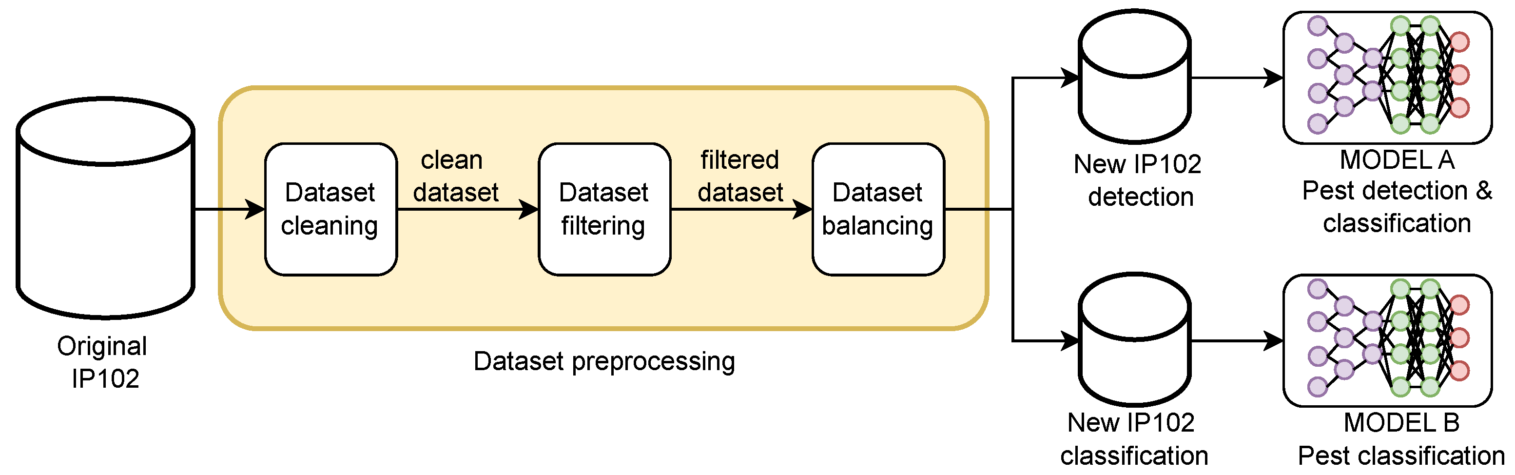
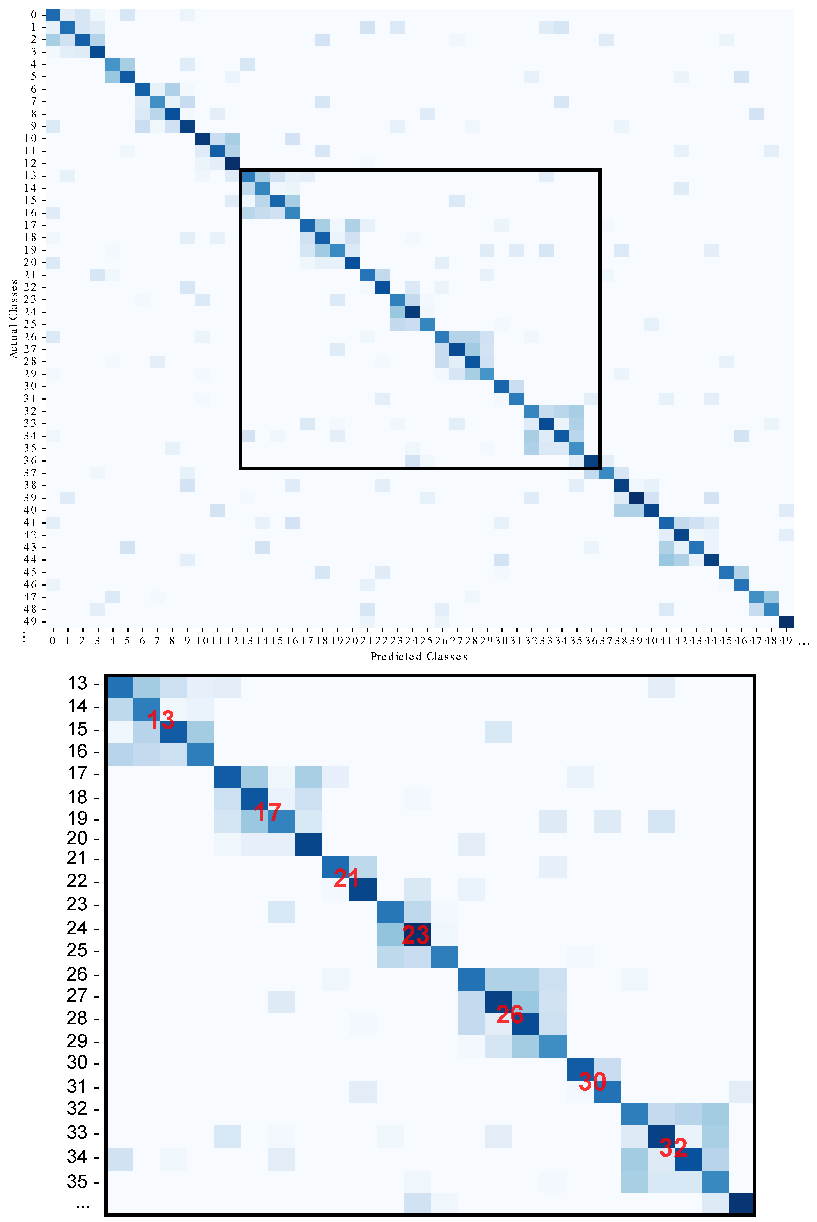
• A novel, general-purpose balancing technique to reduce biasing and variability in the presence of high-unbalanced multi-class datasets is proposed, thus improving classification performance. The designed method is a multi-stage pipeline comprising initial feature analysis, data cleaning, and data filtering steps. The actual balancing process tackles the problem of overnumbered classes by partitioning in multiple subclasses rather than deleting samples, so that the model can still learn from the original feature space. During inference, most of the misclassifications are related to the high correlation between subclasses originated from the same category. The generated confusion matrix will therefore have a block-diagonal trend in which all the errors in a specific sub-block must not be counted as classification errors.
• The construction of a balanced and enhanced version of the IP102 dataset to improve the classification accuracy and robustness of the methods is developed.
• The development of two multi-class insect pest detection and classification models trained on the proposed balanced IP102 dataset is proposed. which reached good performance with challenging images too and outperformed state-of-the-art models trained on the same dataset.

The rest of the paper is organized as follows. Section 2 presents a brief survey of papers concerning both pest classification methods and techniques for data imbalance handling which have been published in the literature in the last five years. In Section 3, the study’s framework is detailed, while in Section 4, the obtained performance is indicated. Finally, some conclusions are drawn in Section 5.

2. Related Studies

Pest detection and classification have become a hot topic in the scientific community because of the increasing attention to the environment and the health and welfare of the individual. The development of Information and Communication Technologies (ITC) has allowed the diffusion of systems and procedures for the semi-automated and automated identification and categorization of insect pests.

This section initially offers an overview of some popular works on the automated localization and identification of pests, which were introduced in the literature in the last five years, and then proposes a review of some of the known techniques used for data imbalanced handling.

2.1. Pest Detection and Classification Frameworks

The lightweight convolutional neural network-embedded attention mechanism characterizes the method indicated in [9], which adopts EfficientNetV2 as a backbone. An efficient attention module is designed by the authors for acquiring channel relationship information and pest positional data from images under testing. However, in [10], the optimization of MobileNetV2 is performed by implementing a dynamic learning rate, freezing layers, and sparse regularization in combination with CutMix augmentation. The MobileNet is also used in [11] as the backbone network for the development of a pest detection system which is based on the Faster Region-based Convolutional Network Method. In the conceived procedure, the ResNet is substituted by the MobileNet to reduce the number of specifications because of the depth-wise separable convolutions used for the MobileNet design. Furthermore, the authors in [12,13] use different convolutional neural network models as classifiers. In particular, pest recognition is carried out after having applied saliency methods for data augmentation in [12], while in [13], transfer learning, fine tuning and CutMix enhancement methods are performed before the classification phase. New residual structures are presented in [14,15,16] based on the fusion feature from previous layers. In particular, Liu et al. [14] thought of merging features from a former layer in the residual signal branch based on the original ResNet for getting more features from the image under test. MobileNetV2, DenseNet121, and InceptionResNetV2 are used in [17] for testing an optimization strategy which uses a genetic algorithm to find the transfer learning and fine-tuning hyperparameters. Long training time, premature convergence, and slow convergent speed are some of the drawbacks encountered during the performance evaluation. To reduce the computational cost and to improve the performance, DenseNet is adopted in [18], which allows the computation of feature maps by linking the output from previous layers as inputs to the following layers.

An ensemble model is conceived in [19] which consists of three pre-trained Convolutional Networks. The output of each of these networks is concatenated for producing a voting classifier ensemble architecture that makes insect classification possible, while in [19], the prediction of the class to which the pest under test belongs is made by hard voting. The authors in [20] adopt a soft voting module for obtaining pest classification. In particular, feature maps are aggregated to produce the activation map for accurate pest detection. Erroneous and unnecessary features are eliminated through the adaptive filtering fusion model by making use of the attention mechanism. Furthermore, an attention mechanism is used in [21] for enhancing the performance of the method, characterized by an architecture based on a spatial transformer network and ResNet.

The authors in [22] have suggested a self-supervised transformer pre-training method for the development of a pest recognition method with better feature representation. A latent semantic mask auto-encoder is proposed, which makes the model capable of learning the semantic features of the pests under test. As the visual transformer architecture is unable to capture the appropriate discriminative information for fine-grained visual classification, the authors in [23] proposed an attention aggregating transformer with an information entropy selector capable of capturing differences between images. Moreover, in [24,25], the extraction of fine grained features is performed by adopting multi-branch and multi-scale learning networks.

A pest recognition based on a single-stage detection-object method is presented in [26,27,28] In more detail, the authors in [26] modify the YOLOv4 backbone network for allowing the extraction of deeper features and improving the recognition rate of densely distributed objects. In [27], a module of the YOLOv5 neck model was changed to process features in a more flexible manner, and an attention mechanism module is introduced for capturing more feature information from the backbone. The classical YOLOv7 approach has been modified in [28] by introducing the Cross-Stage Partial Network as a backbone to enhance feature learning by splitting feature maps and merging them through cross-stage connections. The YOLO algorithm is also used in [29] for the development of a real-time insect classification procedure to be installed on mobile phones. The system was conceived to work both in on-line and off-line modalities so as to monitor farmlands located in limited to no internet/4G/5G connection zones.

For fine-grained image classification processes, an attention-selection mechanism is implemented in [30]. In more detail, An et al. [30] developed a tool which uses a convolutional neural network (CNN) and visual and swin-transformers as backbones for regions of interest localization in the images under test by Gradient-Weighted Class Activation Mapping. Feature extraction from important regions is based on the attention information process and makes the reduction of background noise interference possible. In this way, only local region information of the tested image are necessary, and these are utilized as input to the Support Vector Machine classifier for insect recognition. Furthermore, in [31], a transformer is used to capture global contextual information, thus avoiding the limits of classical convolutional architectures. Unlike the previous study, a non-linear Support Vector Machine classifier with a Power Mean Kernel in combination with fine-tuned EfficientNets are implemented in [32] for the development of a pest classification system. In this way, the training task revolves around the reduction of margin-based loss instead of the decrease in cross-entropy loss.

To improve the method’s robustness in the presence of occluded and distorted images, the authors in [33] conceived a system composed of a global feature extraction network, visual regeneration network, feature fusion module, and a classifier. Patch-based augmentation, pre-trained feature extraction, and distortion information are utilized for achieving the objective. After the creation of an augmented dataset, the visual regeneration network is used for pre-training and capturing low-level semantic features. The fusion of multilevel features coming from the feature extraction and regeneration network makes the model able to accurately recognize insects in real images.

Saliency maps are used in [34,35] for improving the method’s performance. In particular, Bollis et al. [34] have resorted to saliency maps to lead a weakly supervised multiple instance learning method for automatically pinpointing regions of interest in images under test, while Khan et al. [35] adopted fine-grained saliency during the preprocessing phase.

2.2. Techniques for Handling Data Imbalance

The lack of density in the training dataset, the presence of small disjuncts, and the overlap between classes are some of the drawbacks that may arise when dealing with imbalanced datasets [8]. To prevent oversampling methods from adding information to the dataset, the Synthetic Minority Oversampling Technique (SMOTE) was first introduced by Chawla et al. [36]. In this way, the replacement of minority class instances is avoided in favor of the generation of “synthetic” examples. The described method randomly selects a nearest neighbor of a minority instance and linearly generates synthetic examples based on the original instance and a nearest neighbor. Several methods which adopt the SMOTE in combination with other techniques for improving the achieved performance are indicated in the literature [37,38].

Nowadays, with the recent advancements in the field of generative modeling, traditional methods such as SMOTE have been replaced by Generative Adversarial Networks (GANs). In [39], Gurcan et al. have evaluated the effects of introducing GAN-based data augmentation during the training stage of Boosting, Bagging, Linear, and Non-linear classifiers for cancer prediction. The study underlined the struggle encountered by typical models in dealing with imbalance data and highligthed the benefits coming from GAN-based resampling.

A novel data augmentation scheme named the Conditional Generative Adversarial Network Minority-class-augmented Oversampling Scheme (CTGAN-MOS) is introduced in [40] for solving class imbalance problems. The proposed method does not only take into account wrong data distribution, but it also identifies data quality problems. Noisy samples are removed from the starting dataset by means of a coin-throwing algorithm.

Ai et al. [41] claim that most of the existing oversampling methods augment the data by relying only on the intra-class information of minority classes, while ignoring the inter-class relationships with the majority ones. To overcome this, a novel oversampling model is conceived by the authors, named Majority-Guided VAE (MGVAE). MGVAE generates new samples in minority classes under the guidance of a majority-based prior. Therefore overfitting is avoided because new samples inherit the diversity and richness of the majority ones. To account for limited data too, MGVAE is first pre-trained on majority samples and then fine-tuned on minority classes.

The joint problem of data balancing and fairness is analyzed in [42]. Fair OverSampling (FOS) leverages SMOTE to reduce class imbalance and feature blurring to increase group fairness. FOS is designed both to balance the cardinality of classes and to de-bias protected features via feature blurring.

The study carried out in [43] focuses on the effectiveness of GAN-based oversampling methods in tackling the problem of the poor classification performance of minority classes. For this reason, a benchmark is performed among multiple GAN architectures. In more detail, the results achieved by CTGAN, Copula-GAN, WGAN-GP, and DraGAN across classical (KNN, Decision Tree, and Logistic Regression) and ensemble machine learning (XGBoost, Random Forest, and LightGBM) models are compared to identify their strengths and weakness in enhancing classification performance.

3. Materials and Methods

3.1. Pest Image Dataset

The publicly available IP102 dataset is adopted as the reference dataset [44]. The large-scale dataset is composed of more than 75,000 images belonging to 102 different pest categories with a distribution reflecting their presence in nature. The above-mentioned classes are split into 8 crop typologies according to the crop that the insect class damages more (rice, corn, wheat, beet, alfalfa, vitis, citrus, and mango). These typologies are gathered into 2 super-classes based on the kind of corrupted crops called economic and field crops. The dataset contains RGB images at varying pixel resolutions which have been collected from online resources.

The IP102 is a challenging benchmark dataset not only because of its high degree of imbalance but also because images have illumination changes, a broad range of perspective, scale, and orientation. Moreover, several photos are characterized by occlusion and clutter. The difficulty encountered in object detection and recognition in adopting the IP102 dataset is also due to the presence of different pest life stages within the same category (such as larvae, caterpillars, and butterflies).

The dataset provides two options of images and annotations, meant to be used for different pest recognition tasks. In particular, the first collection of 75,222 images can be exclusively used for classification tasks because each image is labeled by species alone and contains a single pest instance. The second collection consisting of 18,976 images features annotations made by specialists which define the bounding box and the class for each instance. This collection is therefore suited for detection and classification tasks.

Given the goal of accurately localizing and classifying insect pests on images captured by in-field sensors, the second collection of the original IP102 dataset has been used in this study for framework development. From now on, the authors refer to this collection as the dataset.

3.2. An Overview of YOLOv8

YOLO is a well-known object detection and classification model, representing the state of the art for real-time and low-resource usage applications. The YOLOv8 model has been developed as an extension of YOLOv5 and is characterized by a modified backbone network, an anchor-free detection head, and a new loss function. The input segment carries out mosaic data augmentation, adaptive anchor calculation, and adaptive grayscale padding on the input image. The backbone makes the extraction of hierarchical features at different scales while the neck aggregates and refines the features extracted by the backbone by focusing on enhancing the spatial and semantic information across different scales [45]. YOLOv8 outperforms its previous versions in terms of mean average precision and performance consistency [46,47,48]. In addition to being faster and more accurate, YOLOv8 also requires fewer parameters to achieve its performance.

A performance comparison of YOLOv8 with newer releases up to YOLOv11, and other architectures like Faster R-CNN, is instead introduced in [49,50], while YOLOv8 is a single-stage object detection model, Faster R-CNN is a two-stage object detection model composed of a Region Proposal Network (RPN) for generating proposals and then doing object detection and classification via bounding box regression. The experimental results confirm YOLOv8’s rapid inference times that make it suitable for real-time applications. It is twice as fast as YOLOv9, while achieving comparable accuracy. Its performance is also comparable with YOLOv10 and YOLOv11. The Faster R-CNN model implemented via Detectron2 instead demonstrated comparatively lower performance in both speed and accuracy compared to the whole family of YOLO algorithms.

3.3. Proposed Method

In this paper, a deep learning-based framework for the detection and classification of different pest species from in-field images is presented. The conceived system is intended to be accurate and characterized by low computational time and cost in order to cope with resource constraints that typically affect in-field sensors and processing platforms. The framework is based on the YOLOv8 architecture, released by Ultralytics in 2023.

Starting from YOLOv8, two models are developed. Model A is conceived to carry out the joint tasks of detection and classification. In particular, the detection phase involves the identification of a bounding box around the detected object (to describe its spatial location) that has to be compared with the ground truth provided in the dataset. After the object localization, model A analyzes the pest in the identified region of interest to classify the insect into predefined categories.

Model B has instead been conceived to perform a pest classification task without any spatial localization, aiming to make a comprehensive comparison with several recent and popular methods indicated in the literature.

The developed methodology is composed of 3 stages (Figure 1). The dataset is acquired and its images undergo a preprocessing phase because of their particular distribution among the different categories. The dataset preprocessing step is shared by the two models. The following sections delve into the details of all the steps that are performed at each stage of the pipeline.

3.3.1. Data Exploration and Data Cleaning

Some data preprocessing techniques are adopted to reformulate the dataset in such a way the deep learning models can learn better. The authors refer to this stage as dataset cleaning and the generated output as the clean dataset.

A preliminary observation of the dataset reveals the following:

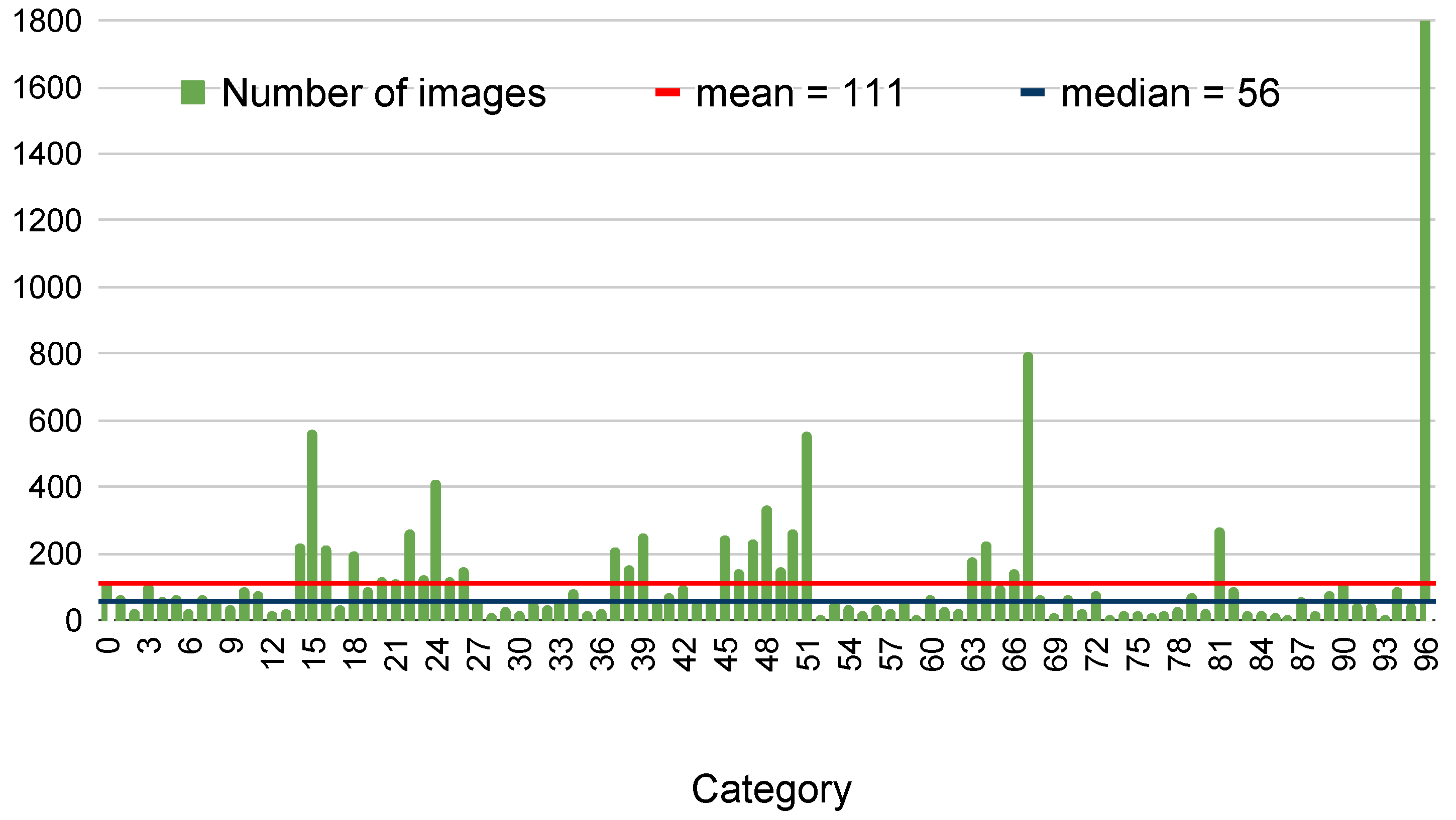
• Pest category distribution is highly unbalanced, ranging from classes with less than 10 samples to classes with more than 1000 samples.
• About $93\%$ of images composing the dataset have a single instance.
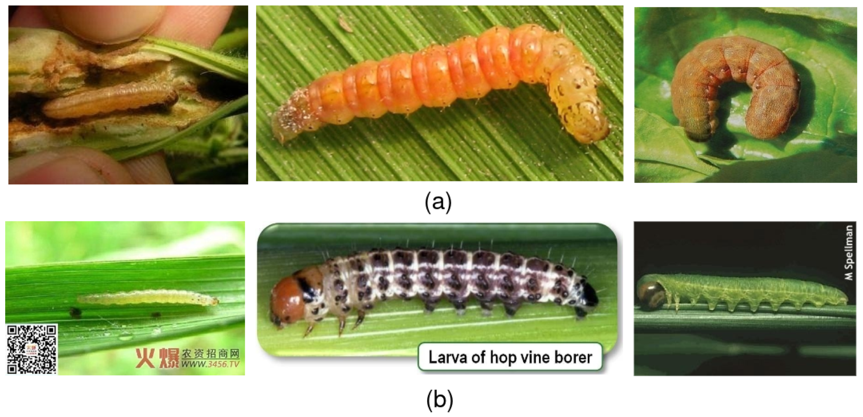
• Different life stages of a specific insect are grouped into the same class.

The consequences of such remarks are as follows:

• Models trained on the dataset as is are likely to become biased towards the majority class and may have trouble generalizing with respect to the less represented classes.
• The detection model will tend to look for a single bounding box on each image under test rather than hunting for a greater number of insect instances as a consequence of the dataset composition.
• There is low similarity between insects belonging to the same class because the same insect can assume very different aspect throughout its lifecycle, thus increasing the in-class variability.
• There is high correlation among dataset categories due to the similar characteristics shared by different insects at the same stage that decrease intra-class diversity.

Figure 2 provides an analysis of the challenges introduced by the IP102 dataset and an overview of the visual features of the samples in the dataset. It is evident that images with a different resolution, size, and condition of acquisition make up the dataset. Figure 2a shows insects belonging to different classes which have very similar physical characteristics, making the discrimination process more difficult. On the contrary, some classes contain images of the same pest in different life-cycle stages (larva, caterpillar, and butterfly) which have different features. Alternatively, in Figure 2b, some samples from the IP102 are indicated which show visual patterns that do not refer specifically to the insect depicted. In fact, the IP102 comprises a lot of samples collected by the internet which report unnecessary writing.

To overcome the above drawbacks, the first strategy proposed by the authors consists of removing all the images with more than one instance from the IP102 dataset. This operation does not have a considerable impact on the dataset’s cardinality (given the low percentage of discarded images) but also makes the dataset suitable for a classification task.

A small $7\%$ of the dataset images with more than one instance is not sufficient to let the model learn to detect more than one insect inside the image under test. The authors have therefore chosen to focus on the accuracy of the detected bounding boxes and on classification performance rather than focusing on the development of a model capable of detecting several instances per image (for which the IP102 dataset is probably not suited).

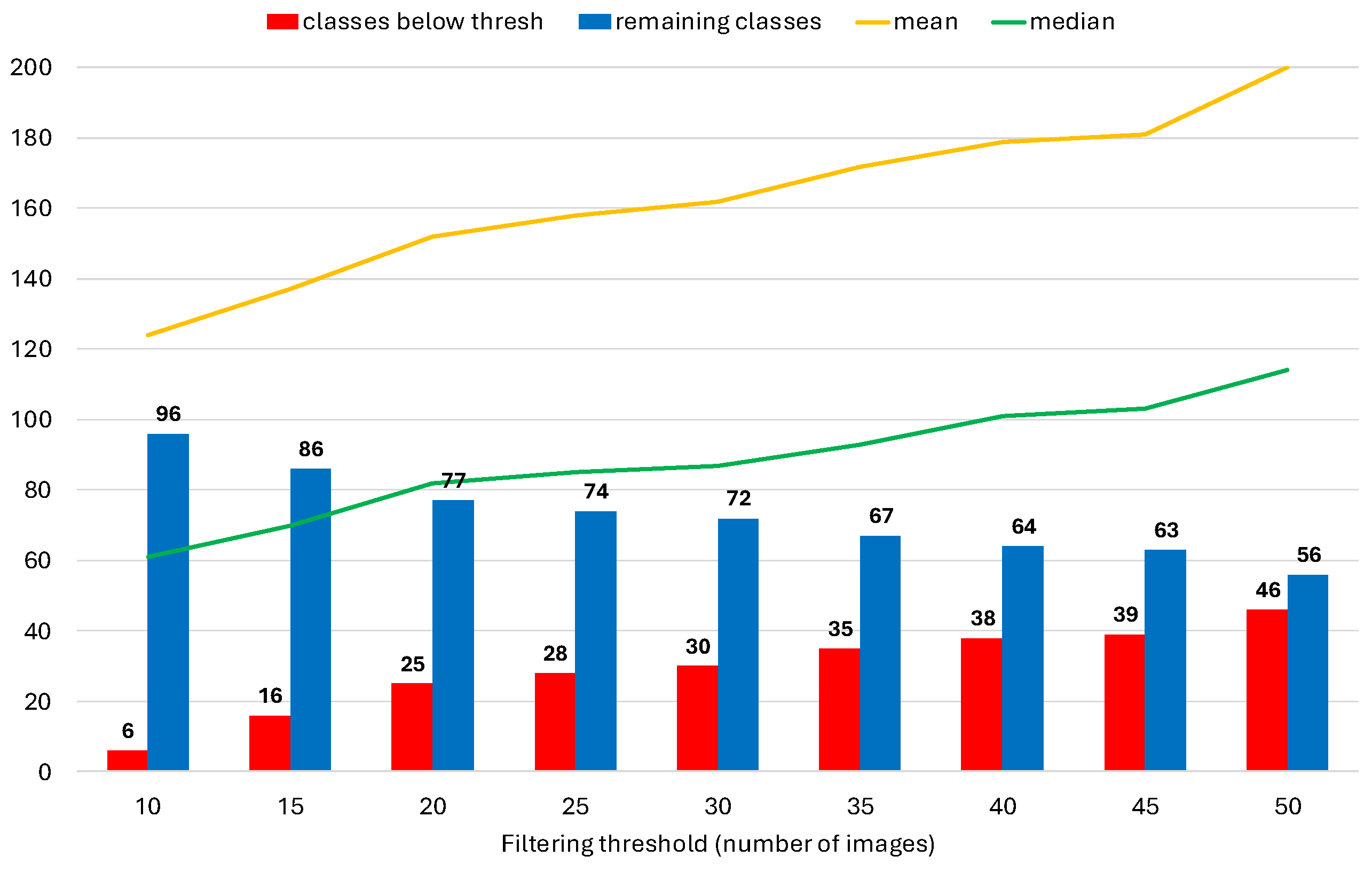
3.3.2. Class-Based Data Filtering

The IP102 dataset, and consequently the obtained clean dataset, is remarkably unbalanced; some classes are even without images. Figure 3 shows the composition of the clean dataset; in particular, the number of samples belonging to each class are indicated, which highlights how the distribution is skewed towards some classes.

Nevertheless, $36\%$ of the clean dataset classes are composed of less than 35 images. A dataset filtering phase is therefore required to ensure that the next data balancing step has a real validity to overcome the unbalanced dataset issue. In fact, augmentation techniques applied to a small set of original images (compared to the median) would produce a large number of synthetic samples which do not provide models with learning features for a proper classification of these pest categories due to overfitting. A fixed threshold for class filtering is therefore employed at this stage with the aim of both maintaining the balanced dataset as close as possible to the original one and maximizing the classification performance. The process of selecting the appropriate threshold has been supported by several experiments.

The objective of this stage is the removal of classes for which a “significant augmentation” is needed so as to avoid the introduction of biases in the dataset. However, a high number of classes in the dataset is composed of few images, and removing all these classes would bias the experiment too. For this reason, several tests have been carried out according to the following approach: $\left(i\right)$ removing classes below a varying threshold, $\left(ii\right)$ checking how many classes and images are remaining, $\left(iii\right)$ applying the augmentation pipeline, and $\left(iv\right)$ checking the classification results. Figure 4 shows the variation of the dataset image distribution with a threshold value as a consequence of the filtering process. An analysis of the figure shows that as the filtering value increases, more classes are removed from the dataset, thus reducing the number of instances for the training phase. As a consequence of the elimination of less populated classes, the median and mean values of the cardinality of the remaining classes increase.

The study carried out has highlighted that a filtering threshold equal to 25 images per class offers an optimal trade-off. In fact, the aforementioned value provides the following: $\left(a\right)$ the removal of classes for which an oversampling procedure would result in the generation of too many synthetic samples; $\left(b\right)$ the maintenance of the majority of classes in the dataset; $\left(c\right)$ the preservation of the scientific validity of the experiment. All classes with a cardinality below 25 are therefore not included in the filtered dataset that undergoes to the next balancing phase.

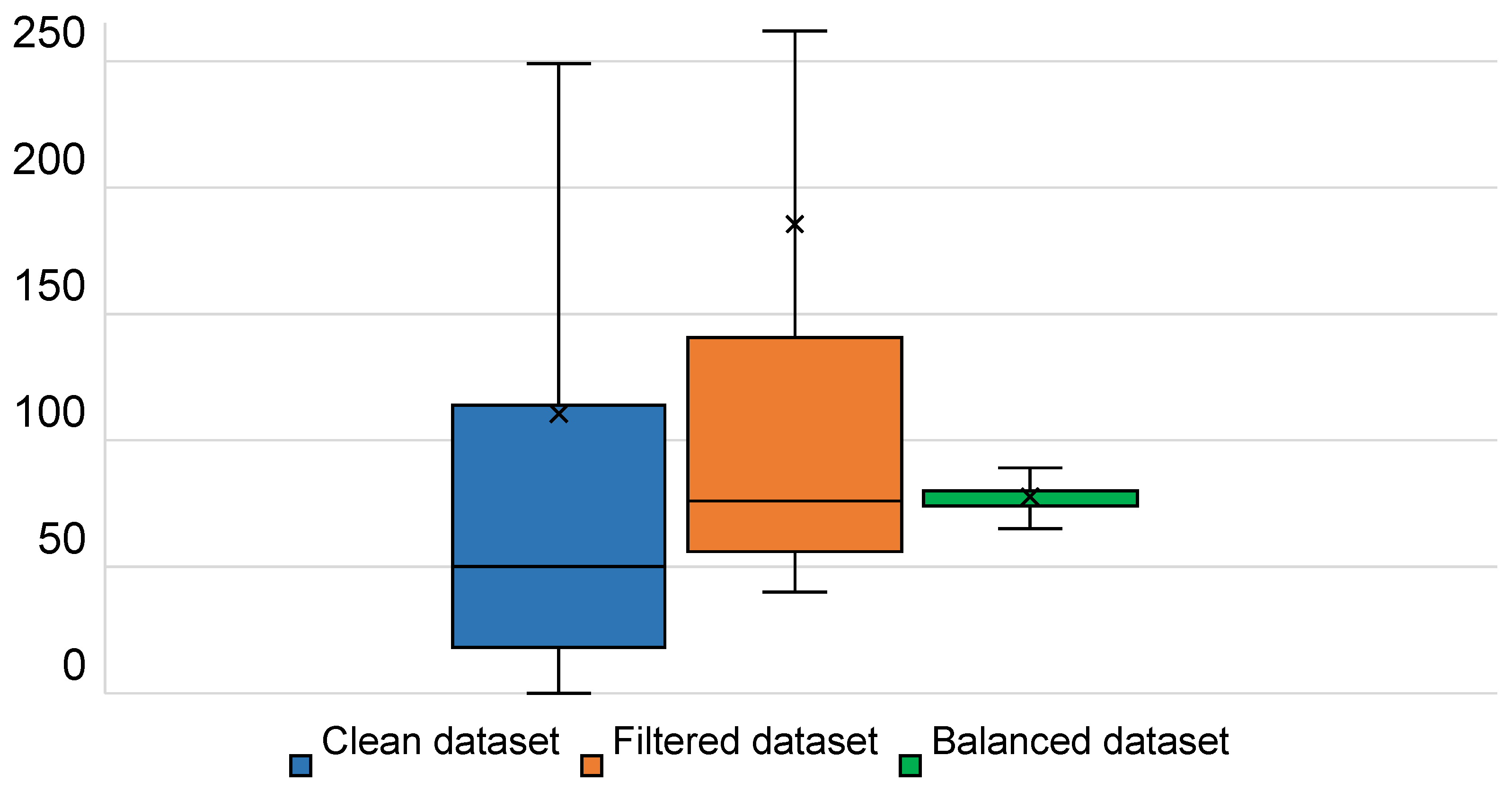
3.3.3. Dataset Balancing

The last step of the proposed method is the dataset balancing process. The filtered dataset still presents a highly unbalanced multi-class distribution. Resampling and data augmentation techniques are usually employed for handling unbalanced datasets.

Data statistics are analyzed to avoid losing relevant data (downsampling) or generating too many artificial samples (upsampling) that may affect the data features. A target number of images per class close to the median value of the filtered dataset has been selected, with a lower bound equal to $75\%$ of the median and an upper bound equal to $150\%$ of the median. These two values define the “acceptance window” and therefore the classes whose cardinality is within this window and do not need modifications. An excessively high lower bound leads to the generation of a large number of synthetic samples that may introduce biases; on the contrary, a lower bound that is too small prevents the usage of data augmentation for oversampling. Given the high number of classes with a cardinality below the median, it has been found that $75\%$ offers the right trade-off between classes that undergo data augmentation and unchanged classes. The value selected for the upper bound has to guarantee that each subcategory coming from the splitting of a class with a significant number of images is still significantly populated for the purpose of the experiment. A median value of $150\%$ ensures that if a class is selected for splitting, all the generated subclasses will have at least 50% of the target images and it is therefore significant for the balancing process.

After selecting the boundaries of the acceptance window, the following rules have been employed:

• Classes with a number of images within the above defined range are left unchanged.
• Classes with a cardinality below the lower bound of the range are upsampled.
• Classes with a cardinality exceeding the upper bound undergo a downsampling process generating new subclasses.

The pseudo-code and the corresponding flow-chart for the balancing procedure are indicated in Algorithm 1 and Figure 5, respectively.

Algorithm 1: Dataset balancing

Figure 5. Flowchart describing the steps of the data balancing process. After defining the median as the ideal number of images per class, each category is processed sequentially. If the number of images is below the given threshold, the category is oversampled by data augmentation (first branch). If the cardinality of the current class is instead over the fixed upper bound, its samples are equally distributed among several subcategories that are created in the new dataset (second branch). Finally, if the cardinality of the current class is within the acceptance window, it is copied as is in the new dataset.

Figure 5. Flowchart describing the steps of the data balancing process. After defining the median as the ideal number of images per class, each category is processed sequentially. If the number of images is below the given threshold, the category is oversampled by data augmentation (first branch). If the cardinality of the current class is instead over the fixed upper bound, its samples are equally distributed among several subcategories that are created in the new dataset (second branch). Finally, if the cardinality of the current class is within the acceptance window, it is copied as is in the new dataset.

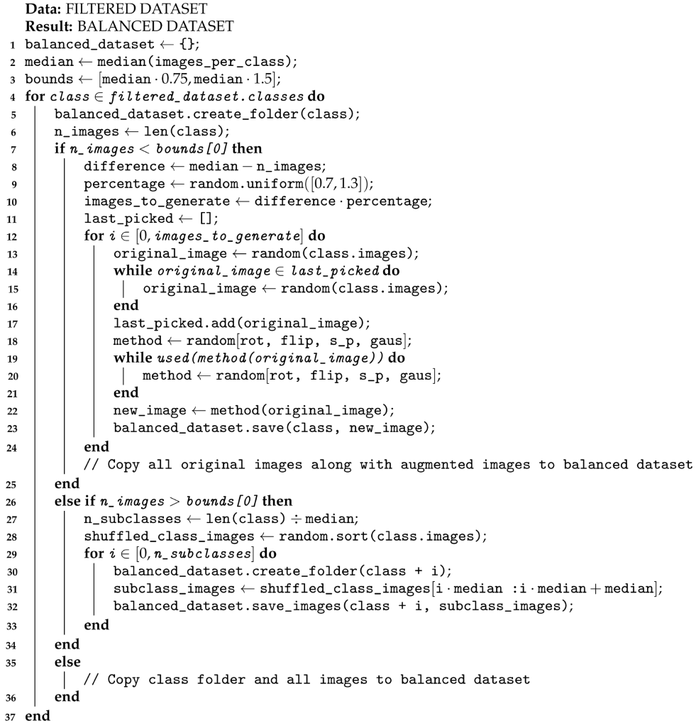
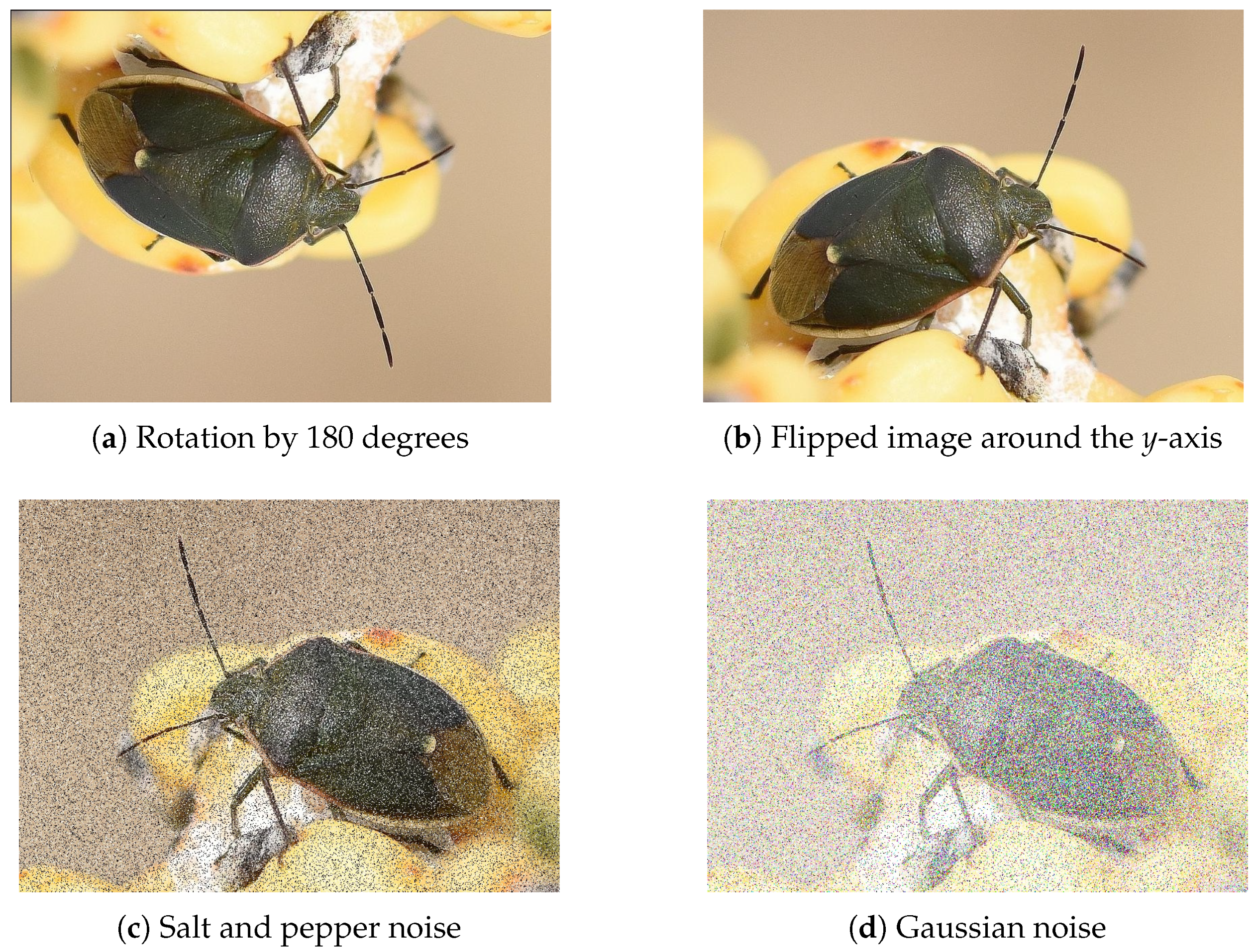
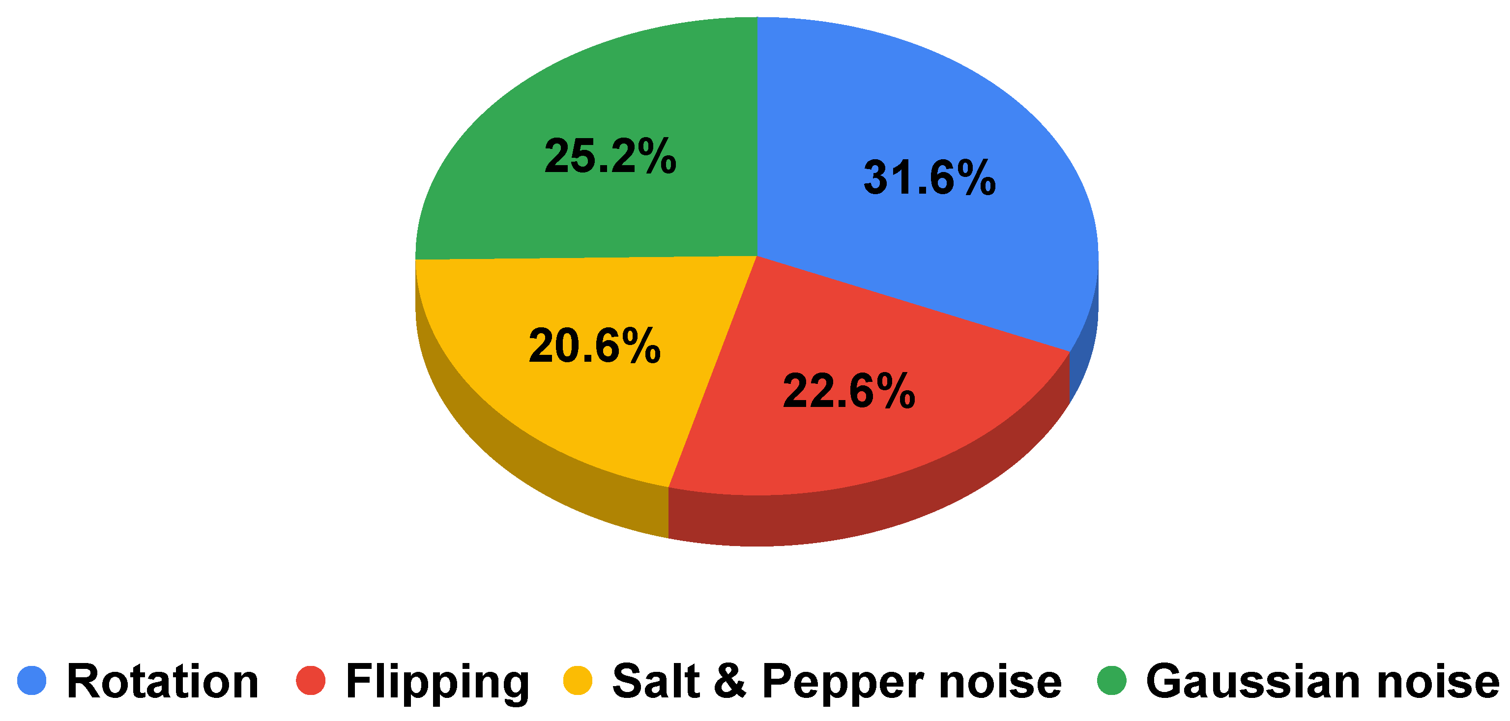
Upsampling Processing Technique

Let class $\alpha$ be a generic class of the filtered dataset for which upsampling is necessary. The designed procedure defines in advance the number of images that will compose class $\alpha$ at the end of the procedure, by picking up a random number in the range between $\pm 30\%$ of the median value. By doing so, it is ensured that the cardinality of all the upsampled classes of the filtered dataset will be around the median.

An image $I_{\alpha }$ of class $\alpha$ is randomly selected to increase the data. The particular augmentation technique to apply to $I_{\alpha }$ is then randomly selected among the following options:

• Rotation with a random angle between 90, 180, and 270. The values of the angles are fixed to avoid the creation of blank spaces in the corners of the image.
• Flipping along the randomly selected axis.
• Gaussian noise addition, with a mean of 0 and std of 10.
• Salt and pepper noise addition, with a random number of pixels between $20\%$ and $30\%$ of the total number of pixels, equally distributed between black and white noise.

The choice of using only 4 augmentation techiniques works for the purpose of this paper, which is to investigate whether the classification problem can benefit from an appropriate balancing technique and not studying how augmentation techniques affect the classification problem.

To prevent the framework from producing identical images during augmentation, the implemented procedure always checks that $I_{\alpha }$ has not been used to produce one of the last 20 augmented images and that the chosen augmentation tool has not been previously used on $I_{\alpha }$. The above-mentioned data augmentation procedure has to be carried out N times with N equal to the number of images to be added to class $\alpha$ for dataset balancing.

Figure 6 shows some examples of augmented images which were produced from generic images from the filtered dataset.

Downsampling Processing Technique

Typical downsampling approaches involve the removal of excessive images. A novel approach for data balancing without sample scraping is indicated in this paper. Let class $\beta$ be a generic class of the filtered dataset for which downsampling is necessary. The conceived technique provides that class $\beta$ is split into several sub-classes with an equal number of images. The number of sub-classes generated by class $\beta$ is computed as the ratio between the cardinality of $\beta$ and the median of the filtered dataset. Images belonging to class $\beta$ are then distributed in each obtained sub-class by choosing to perform an additional shuffling procedure at random intervals.

During the step of splitting the generic class $\beta$ into multiple sub-classes, a json file keeping track of the associations between the original class $\beta$ and all the generated sub-classes is created. These associations are then used for the evaluation of the classification performance. A classification error does not occur if an image belonging to class $\beta$ is misclassified and assigned to a sub-class of $\beta$.

By adopting the proposed approach, the representation and interpretation of the confusion matrix also change. The confusion matrix, usually representing a diagonal pattern, is characterized by a diagonal-block distribution, since the majority of classification errors represent instances of class $\beta$ predicted as one of its sub-classes. When computing the performance scores, all the misclassified instances falling in the sub-block of class $\beta$ must not be interpreted as errors.

The output of the balancing process is named the balanced dataset and represents the input for the next steps of the designed methods.

Figure 7 shows the distribution of images per category and highlights how intra-class imbalances are reduced by using the proposed procedure.

3.3.4. Model Design

For pest detection and classification, the YOLOv8 architecture is adopted. It is based on an anchor-free model with a decoupled head to process objectness, classification, and regression tasks independently. The scalability and modularity of the YOLOv8 architecture make its design easily customizable in terms of parameter characteristics such as anchor boxes, input size, and complexity. This hierarchical architecture provides the ability to learn many object classes and to accurately detect objects in challenging images too [51]. It is a fast one-stage object detection procedure which is characterized by an input segment, a backbone, a neck, and an output segment [45]. The input segment carries out mosaic data augmentation, adaptive anchor calculation, and adaptive grayscale padding on the input image. The backbone carries out the extraction of hierarchical features at different scales while the neck aggregates and refines the features extracted by the backbone by focusing on enhancing the spatial and semantic information across different scales. Multiple Conv and C2F (cross-stage partial bottleneck with two convolutions) modules process the input image for feature extraction maps at diverse scales. The output feature maps are analyzed by the Spatial Pyramid Pool Fusion (SPPF) module, which performs pooling with different kernel sizes. The obtained results are fed as input to the neck layer which incorporates the Path Aggregation Network (PANet) and Feature Pyramid Network (FPN) to improve the feature fusion procedure. The detection part of Yolov8 distinguishes the classification head from the detection head (bounding box regression). Binary cross-entropy loss (BCE Loss) and distribution focal loss (DFL) with complete intersection over union (CIoU) are employed as the loss functions for classification and detection tasks, respectively, [52]. Starting from YOLOv4, MOSAIC data augmentation has been introduced in the training pipeline. This technique is an improvement of the Cutmix augmentation, in which 4 training images are combined into a single one [53]. In more detail, MOSAIC resizes each of the 4 images, creates the combined image, and finally takes a random cutout to obtain the final image. The final image could therefore contain only small portions of original images and objects. MOSAIC is used to help the model generalize and avoid overfitting, since it is forced to also recognize objects from partial views with reduced features.

3.4. Setup and Strategy

The proposed approach was implemented in a Python 3.9 environment running under the Ubuntu 20.04 operating system. The testing machine was equipped with an Intel Core i7-9700K @ 3.60 GHz processor, 16 GB RAM, and 24 GB NVIDIA GeForce RTX 4090 graphics processing unit, running CUDA 12.1.

To train and deploy the proposed pipeline, the PyTorch 2.1.2 module—on top of which the YOLOv8 model is defined—is the only software requirement. Alternatively, the Ultralytics library installs all the required modules. Each parameter of the YOLO model can be customized. RGB images with a $640\times 640$ pixel resolution are used for enhancing the model capability to capture small details that could be relevant for the accurate classification. The pre-trained weights are used to leverage the ability of the model to extract relevant features.

Table 1. Training parameters for the (i) classification model and (ii) detection and classification model.

YOLOv8 Parameters	Classification Model	Detection and Classification Model
Image size	640	640
Batch size	32	24
Epochs	1000	1000
Pre-trained	True	True
Optimizer	SGD	SGD
Early stopping	Disabled	Disabled
Learning rate	0.01	0.01
Momentum	0.937	0.937
Weight decay	0.0005	0.0005
Augment	False	False
Mosaic	False	False
Translate	0.0	0.0
Flipud	0.0	0.0
Fliplr	0.0	0.0
Hsv_h	0.0	0.015
Hsv_s	0.0	0.7
Hsv_v	0.0	0.4
Degrees	0.0	-
Scale	0.0	-
Shear	0.0	-
Perspective	0.0	-
Mixup	False	-
Erasing	0.0	-

lists all the parameters that have been used to train both designed models.

The original training and testing data ratio of the IP102 pest detection datasets is 80:20, with a total number of 15178 images for training and 3798 in the testing split. After the dataset balancing process, the ratio is 85:15, as the testing images are not modified while the training set size is increased. Figure 8 shows the distribution of the augmented images of the training set as a function of the specific technique implemented for their generation.

3.5. Evaluation Metrics

For the effectiveness assessment of the method, Recall (R), Precision (P), F1-score, Intersection over Union (IoU), and Accuracy are evaluated according to Equations (1)–(5):

$$R={\displaystyle \frac{TP}{TP+FN}}$$

(1)

$$P={\displaystyle \frac{TP}{TP+FP}}$$

(2)

$$Acc={\displaystyle \frac{TP+TN}{TP+FP+TN+FN}}$$

(3)

$$F{1}_{score}=2·{\displaystyle \frac{P·R}{P+R}}$$

(4)

$$IoU={\displaystyle \frac{A\cap B}{A\cup B}}$$

(5)

where TP (True Positives) is the number of correct identifications of instances inside the image under test, FN (False Negatives) is the number of instances present in the image that the algorithm does not recognize, FP (False Positives) is the number of predictions misclassified as instances in the image, and TN (True Negatives) is the number of predictions correctly classified as negative. A is the predicted bounding box and B is the ground truth bounding box.

4. Experimental Results and Analysis

This section discusses the details of the experimental setup, the training strategy and the adopted evaluation metrics first. After that, the performance analysis and comparisons with the state of the art are described to prove the efficiency of the conceived system.

4.1. Performance Analysis and Comparison

This section presents the performance analysis of the conceived method. The IP102 dataset is adopted as a test bench for models performing a challenging task on images with a complex background, different light conditions, and multi-distances and multi-angles views. The results of the detection and classification model and the classification-only architecture are compared to state-of-the-art models from the literature.

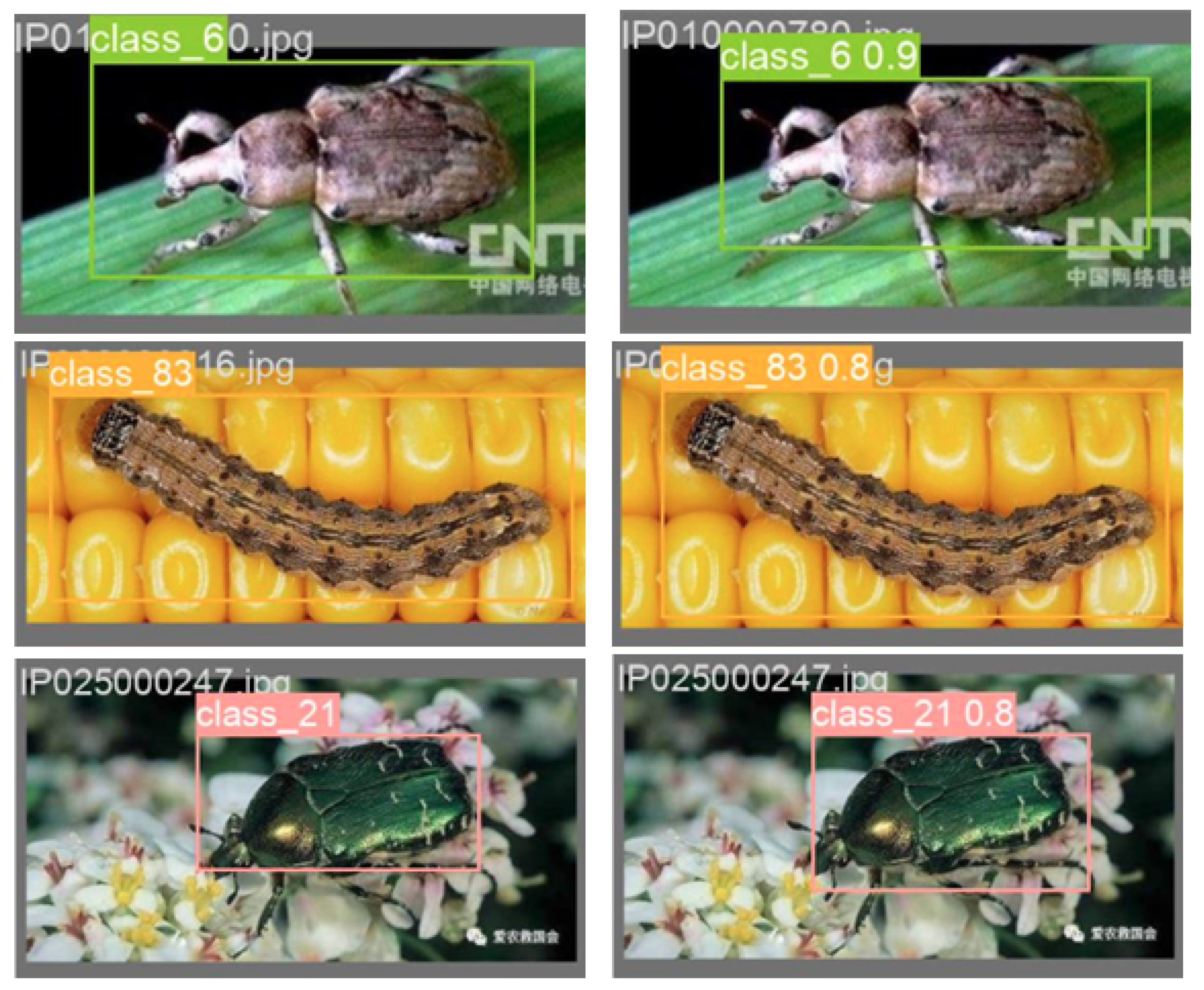
4.1.1. Pest Detection and Classification Results

For multi-class pest detection and classification, model A is adopted. Figure 9 shows some examples of pest detection and classification results using the proposed model. The obtained results underline the validity of the method in locating pests, even if challenging images are tested. In fact, pests of varying sizes, shapes, and colors are accurately located.

In

Table 2. Detection and classification performance comparison.

	Acc	F1	IoU	P	R
[18]	68.74	59.39	0.621	61.72	57.46
[27]	-	57.50	-	57.40	-
Our method	74.77	78.63	0.79	82.25	74.76

, the ability of model A to localize pest and then recognize the insects inside the bounding box is indicated and compared with other recent methods indicated in the literature. Among all the recently released methods adopting the IP102 dataset as a test bench, the comparison takes into account only frameworks performing both detection/localization and classification tasks.

4.1.2. Pest Classification Results

The high capacity to correctly classify different species of pests is of key importance for the reliability of the method. To this aim, model B is considered. Figure 10 shows the confusion matrix plot of the designed method that highlights the performance of pest classification in terms of predicted and actual classes. The TP values for each class are reported along the diagonal of the confusion matrix. The higher the accuracy value of the classification task, the darker the color of the diagonal. The process of distributing overnumbered samples into several subcategories leads to the generation of highly correlated classes. The model benefits from an equal data distribution but struggles to make the correct subclass prediction in case of samples generated from the same original class (having, therefore, common visual features). This trend is shown in the diagonal-block distribution of the confusion matrix as follows (Figure 10): each sub-block along the diagonal contains all the classification errors generated when the model confuses the original class with one of the generated subclasses. The bigger the block, the higher the number of the subclasses generated by the proposed method. However, these errors must not be considered as actual misclassifications in the performance evaluation phase because those instances belong to the same class in the original dataset, regardless of the subclass they belong to after balancing. For the sake of visualization, only a portion of the confusion matrix is reported in the figure. In the enlarged view, all the categories falling in each sub-block along the diagonal actually belong to the pest class highlighted in red. The color gradation shows the magnitude of the classification errors as follows: the darker the color, the higher the number of misclassified instances.

In

Table 3. Detection and classification performance comparison.

	Acc %	F1	P	R	Y	T
[9]	73.7	-	-	-	2023	Lightweight CNNs + embedded attention
[10]	71.32	-	-	-	2021	Lightweight CNNs + embedded attention
[11]	82.43	82	83	81	2023	Faster-RCNN + MobileNet
[12]	61.93	59.2	-	-	2020	Saliency + CNNs
[13]	86.95	-	-	-	2023	ResNeXt-50
[14]	55.43	54.18	-	-	2022	Residual Network (DFF-ResNet)
[15]	55.24	54.18	-	-	2019	Residual network (FR-ResNet)
[16]	52.32	-	-	-	2020	ExquisiteNet
[17]	71.48	64.06	65.85	63.22	2024	Pre-trained CNN + genetic algorithm
[19]	82.5	-	-	-	2023	3 pre-trained CNNs
[20]	73.9	73.6	-	-	2023	CNN + EFLM + AFFM
[21]	73.29	-	-	-	2021	CNN+ spatial attention
[22]	74.69	74.36	-	-	2022	Self-supervised transformer
[23]	75	-	-	-	2023	Attention aggregating transformer
[24]	74.20	-	-	-	2023	CNN + improved Vision Transformer
[25]	78.15	-	-	69.24	2025	Channel-Enhanced and Multi-Scale
[27]	-	57.5	57.4	-	2023	Improved yolov5 architecture
[28]	-	-	85.55	84.25	2025	Modified yolov7
[30]	65.6	60.3	60.9	59.7	2023	CNN ResNet + attention Vision Transformer
[31]	75.74	-	-	-	2024	CNN + Transformers
[32]	72.31	-	-	-	2023	Fine-tuning EfficientNets + SVM
[33]	68.34	68.34	68.37	68.33	2024	Visual regenerative fusion network
[34]	60.7	59.6	-	-	2020	Multiple-Instance LCNN
[35]	81.7	-	-	-	2022	InceptionV3
Our method	88.34	87.86	88.67	86.34	-	-

, a comparative analysis of the performance achieved by model B in the classification task is summarized with the findings of other techniques indicated in the literature that adopt the same dataset as the test bench. The methods taken into account for the benchmarking have been detailed in Section 2. The results of the method validate the performance of model B.

4.2. Model Robustness

Finally, the robustness of the developed models has been assessed. While the images in the IP102 contain clear, high-resolution acquisitions of pests, images acquired by in-field sensors may be affected by reduced resolution due to the resource constraints of low-power sensors. Moreover, dust, rain, and terrain particles may dirty the image and cover parts of the pests being acquired. In some cases, in-field sensors are only responsible for data acquisition and transmission to remote stations where the detection and classification models are executed. Due to the low resource usage and network bandwidth constraints, the pictures acquired on the field sometimes need to be downsampled in order to be transmitted over the network.The purpose of this study is to stress the conceived models under real-world conditions. The proposed levels of added noise have been chosen to cover the entire 100% interval in a few steps. In this way, an idea is given of the performance degradation the network can face during the training phase in the case of low signal-to-noise ratio in the acquisition system, The case for the resolution has also been addressed with the same approach.

For this reason, the study aims to evaluate the robustness of the model to decreasing levels of image resolution and to increasing levels of pixel-wise noise.

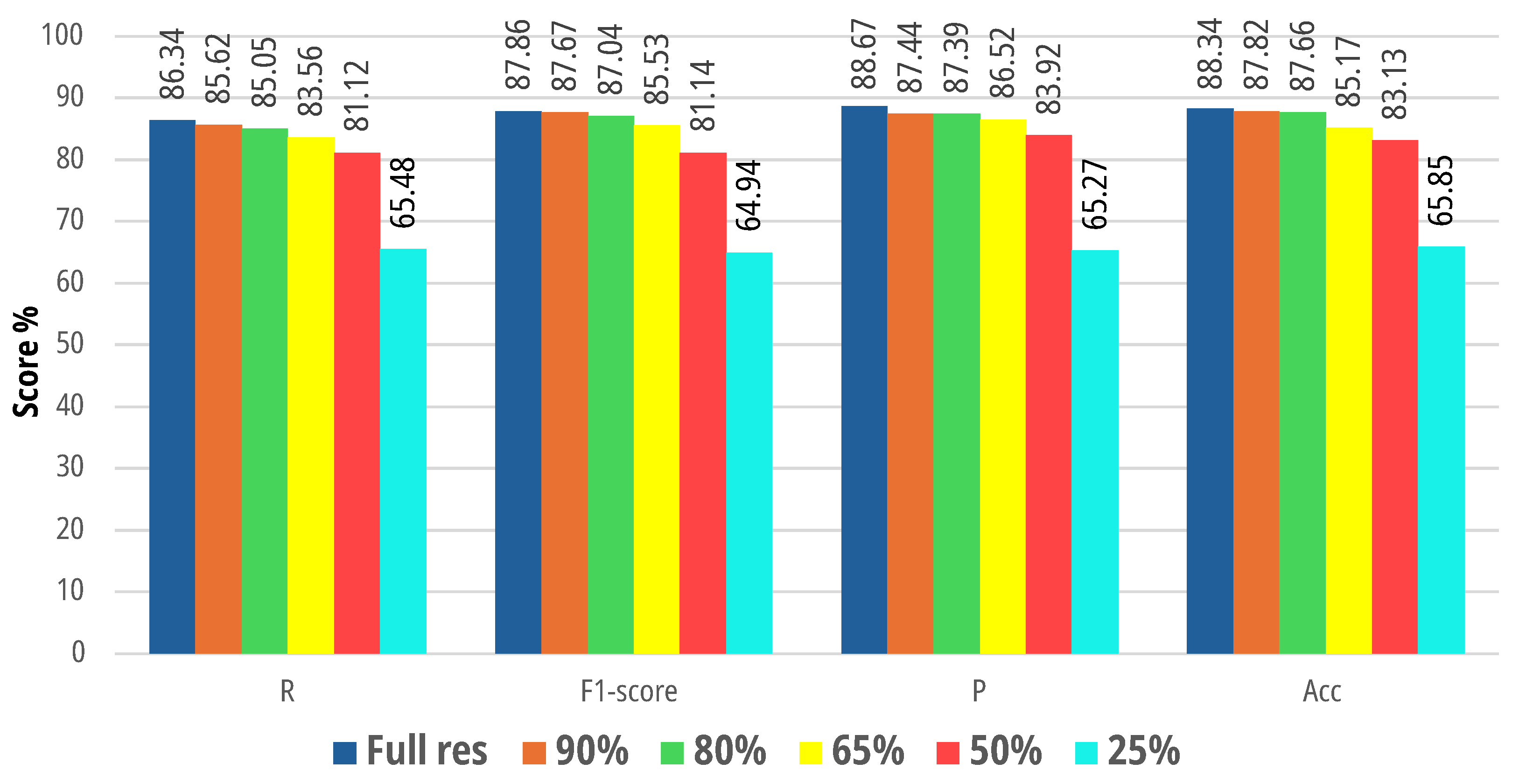
4.2.1. Robustness of the Designed System to Image Resolution

In this study, the whole test set of the IP102 dataset is adopted as a test bench. Five image datasets with different resolutions are generated to evaluate the influence of the resolution factor on the method performance. The five datasets are composed of the same images (all the images of the IP102 test set) but they differ in image resolution value. Denoting with $\mathtt{res}$ the resolution of the images of the IP102 test set, the five datasets are composed of images with a resolution equal to $90\% \mathtt{res}$, $80\% \mathtt{res}$, $65\% \mathtt{res}$, $50\% \mathtt{res}$, and $25\% \mathtt{res}$, respectively.

Figure 11 and Figure 12 show the robustness against resolution degradation of model A and model B, respectively.

By analyzing the obtained results, the ability of both model A and model B to maintain adequate performance even under extreme conditions due to the low quality images adopted as the test bench is highlighted.

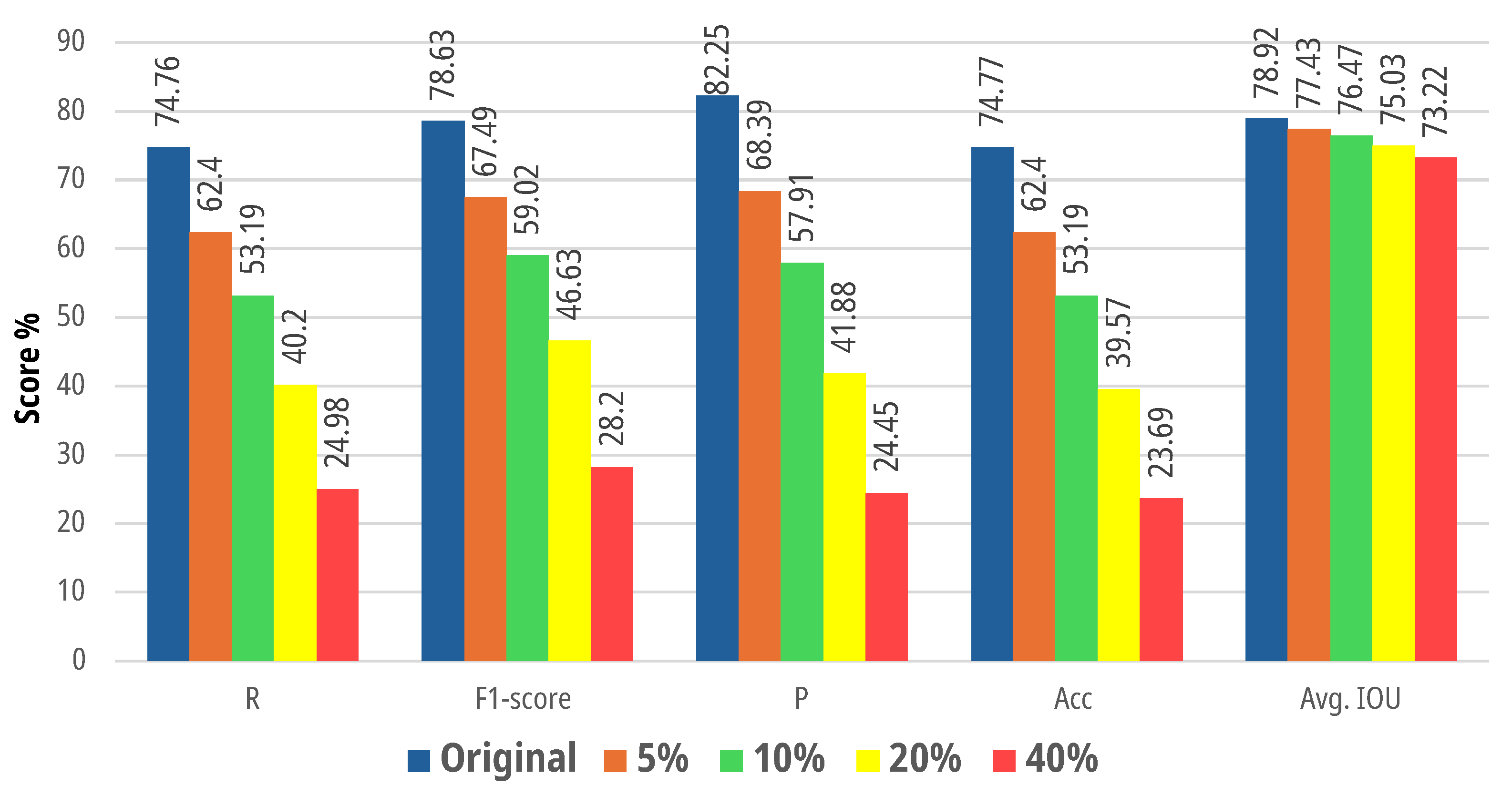
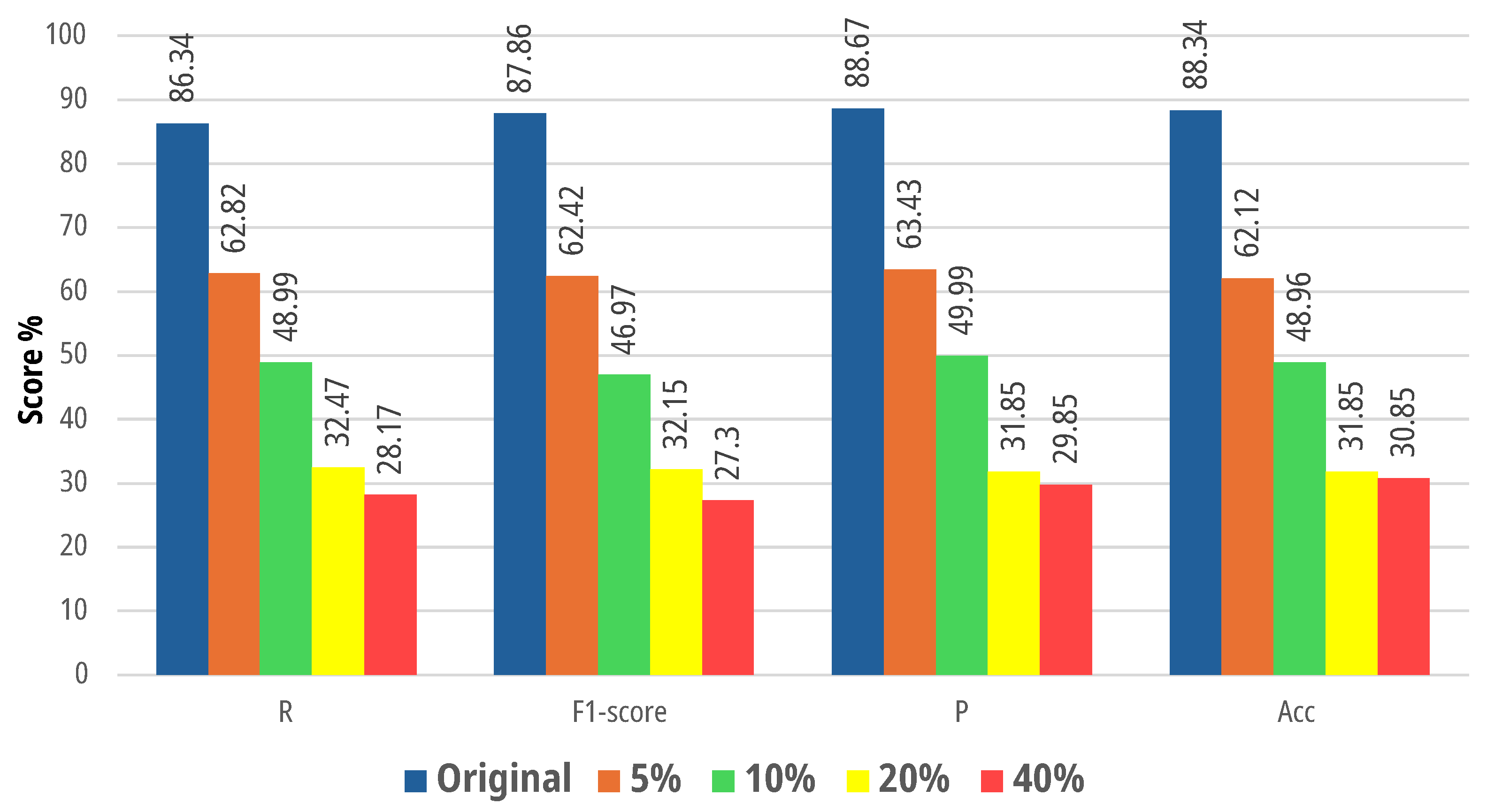
4.2.2. Robustness of the Designed Systems to Noise

The corruption of the signal with noise is typical in signal processing for simulating different and possible situations that may realistically arise, such as interferences, distortions, and so on. These situations could result from the poor performance of the capturing device or from specific environmental conditions. For this analysis, salt and pepper noise is added so a certain amount of pixels in the image is randomly digitalized with maximum or minimum intensity. Therefore, salt and pepper noise results in randomly dotted pictures with white and black pixels in the image [54,55].

For the noise robustness evaluation of the implemented models, the whole test set of the IP102 dataset is adopted as a test bench. Four image datasets, each with a different amount of pixel corrupted by noise, are considered. The four datasets are composed of the same images (all the images of IP102 test set) but they differ in the percentage of noise added to images. Let $\mathtt{px}$ be the number of pixels making up the images of the IP102 test set and $\delta \% \mathtt{px}$ the percentage of image pixels corrupted by pepper and salt noise; the four datasets adopted consist of images with $\delta$ equal to 5, 10, 20, and 40, respectively.

The results, shown in Figure 13 and Figure 14, highlight the performance of methods A and B versus the amount of added noise.

Compared to downsampling, the performances of the developed models drop more rapidly as a consequence of pixel-wise alterations. This is justified by the fact that downsampling operations reduce the image quality but do not affect the visual features of pests, so the model is still able to detect and classify even under challenging conditions. Salt and pepper noise instead forces pixels to change their original color intensity, thus affecting the visual features of the pest in the image. As a consequence, the model struggles to classify pests in the proper way.

5. Conclusions

Pest detection and identification is a critical activity in open fields because of the presence of a complex background in the captured image, different light conditions, and the varying postures and sizes of the same insect due to the multi-distance and multi-angle views in image capturing. Unfortunately, prompt action is required where a pest attack is taking place because of the rapid spread of the infestation. It is evident that one of the most effective strategies for pest control is the accurate and timely pest detection. Artificial Intelligence techniques and Information and Communication Technologies are playing an ever-increasing role in smart agriculture, offering solutions to several problems like pest management, smart irrigation, and so on.

Nevertheless, the performance of deep learning models depends on several factors like model complexity compared to data distribution, training data quality and quantity, hyperparameter tuning, and many others. When developing applications for real-world scenarios, one of the key requirements for training data is to closely reflect the real-world data distribution to avoid any performance degradation when deploying the model with in-field collected data. However, real-world data rarely have a uniform distribution, and this aspect is reflected in the strong imbalance of the datasets. Data imbalance is a challenging problem because it leads the model to prefer the most represented classes, while struggling to extract relevant information from the minority ones. The most widely adopted techniques in the literature involve resampling techniques based on augmentation and downsampling. The latter causes data deletion and the loss of useful information.

To avoid any loss of information and to reduce biasing in the presence of high-unbalanced multi-class datasets, a novel data balancing technique is introduced in this work. The idea is to preserve dataset expressiveness by avoiding sample removal from overnumbered classes and, at the same time, reduce the generation of synthetic samples. For this aim, supernumerary classes are split into several subsequent sub-classes for balancing the representativeness of each category in the dataset without deleting any sample.

The proposed approach is context-free and can be used to tackle the biasing problem with any kind of dataset.

To evaluate the efficacy of the proposed method, a framework for the automatic localization and classification of several crop pests in outdoor conditions is also indicated. The method is based on deep learning strategies and is computationally efficient. The system’s effectiveness is validated, taking into account a freely available database composed of challenging images as the test bench. The obtained results highlight the method’s validity and its immunity towards resolution degradation. Future studies include the development of a special-purpose system which will integrate the procedure detailed above. The system will also be equipped with suitable hardware devices and software tools for image acquisition, processing, and transmission to a remote platform in charge of collecting and displaying the received data. Data gathered will be managed to analyze the growth rate of the infestation and to take prompt measures to tackle the pest problem. Moreover, future developments will investigate both the method’s performance on various datasets from different domains and the possibility to adopt the proposed approach with non-image-based datasets. In addition, special care will be taken to verify the possibility to integrate learning-based methods capable of selecting the images to cut out.

References

1. Puliga, G.A.; Sprangers, T.; Huiting, H.; Dauber, J. Management practices influence biocontrol potential of generalist predators in maize cropping systems. Entomol. Exp. Appl. 2024, 172, 132–144. [Google Scholar] [CrossRef]
2. Coulibaly, S.; Kamsu-Foguem, B.; Kamissoko, D.; Traore, D. Deep learning for precision agriculture: A bibliometric analysis. Intell. Syst. Appl. 2022, 16, 200102. [Google Scholar] [CrossRef]
3. Mamdouh, N.; Wael, M.; Khattab, A. Artificial intelligence-based detection and counting of olive fruit flies: A comprehensive survey. In Cognitive Data Science in Sustainable Computing; Deep Learning for Sustainable Agriculture; Academic Press: Cambridge, MA, USA, 2022; pp. 357–380. [Google Scholar] [CrossRef]
4. Karlsson Green, K.; Stenberg, J.A.; Lankinen, Å. Making sense of Integrated Pest Management (IPM) in the light of evolution. Evol. Appl. 2020, 13, 1791–1805. [Google Scholar] [CrossRef] [PubMed]
5. Lello, F.; Dida, M.; Mkiramweni, M.; Matiko, J.; Akol, R.; Nsabagwa, M.; Katumba, A. Fruit fly automatic detection and monitoring techniques: A review. Smart Agric. Technol. 2023, 5, 100294. [Google Scholar] [CrossRef]
6. Preti, M.; Verheggen, F.; Angeli, S. Insect pest monitoring with camera-equipped traps: Strengths and limitations. J. Pest Sci. 2021, 94, 203–217. [Google Scholar] [CrossRef]
7. Teixeira, A.C.; Ribeiro, J.; Morais, R.; Sousa, J.J.; Cunha, A. A systematic review on automatic insect detection using deep learning. Agriculture 2023, 13, 713. [Google Scholar] [CrossRef]
8. Spelmen, V.S.; Porkodi, R. A review on handling imbalanced data. In Proceedings of the 2018 International Conference on Current Trends Towards Converging Technologies (ICCTCT), Coimbatore, India, 1–3 March 2018; pp. 1–11. [Google Scholar] [CrossRef]
9. Zheng, T.; Yang, X.; Lv, J.; Li, M.; Wang, S.; Li, W. An efficient mobile model for insect image classification in the field pest management. Eng. Sci. Technol. Int. J. 2023, 39, 101335. [Google Scholar] [CrossRef]
10. Setiawan, A.; Yudistira, N.; Wihandika, R.C. Large scale pest classification using efficient Convolutional Neural Network with augmentation and regularizers. Comput. Electron. Agric. 2022, 200, 107204. [Google Scholar] [CrossRef]
11. Ali, F.; Qayyum, H.; Iqbal, M.J. Faster-PestNet: A Lightweight deep learning framework for crop pest detection and classification. IEEE Access 2023, 11, 104016–104027. [Google Scholar] [CrossRef]
12. Nanni, L.; Maguolo, G.; Pancino, F. Insect pest image detection and recognition based on bio-inspired methods. Ecol. Inform. 2020, 57, 101089. [Google Scholar] [CrossRef]
13. Li, C.; Zhen, T.; Li, Z. Image classification of pests with residual neural network based on transfer learning. Appl. Sci. 2022, 12, 4356. [Google Scholar] [CrossRef]
14. Liu, W.; Wu, G.; Ren, F.; Kang, X. DFF-ResNet: An insect pest recognition model based on residual networks. Big Data Min. Anal. 2020, 3, 300–310. [Google Scholar] [CrossRef]
15. Ren, F.; Liu, W.; Wu, G. Feature reuse residual networks for insect pest recognition. IEEE Access 2019, 7, 122758–122768. [Google Scholar] [CrossRef]
16. Zhou, S.Y.; Su, C.Y. Efficient convolutional neural network for pest recognition-ExquisiteNet. In Proceedings of the 2020 IEEE Eurasia Conference on IOT, Communication and Engineering (ECICE), Yunlin, Taiwan, 23–25 October 2020; pp. 216–219. [Google Scholar] [CrossRef]
17. Ayan, E. Genetic algorithm-based hyperparameter optimization for convolutional neural networks in the classification of crop pests. Arab. J. Sci. Eng. 2024, 49, 3079–3093. [Google Scholar] [CrossRef]
18. Albattah, W.; Masood, M.; Javed, A.; Nawaz, M.; Albahli, S. Custom CornerNet: A drone-based improved deep learning technique for large-scale multiclass pest localization and classification. Complex Intell. Syst. 2023, 9, 1299–1316. [Google Scholar] [CrossRef]
19. Anwar, Z.; Masood, S. Exploring deep ensemble model for insect and pest detection from images. Procedia Comput. Sci. 2023, 218, 2328–2337. [Google Scholar] [CrossRef]
20. Chen, Y.; Chen, M.; Guo, M.; Wang, J.; Zheng, N. Pest recognition based on multi-image feature localization and adaptive filtering fusion. Front. Plant Sci. 2023, 14, 1282212. [Google Scholar] [CrossRef]
21. Yang, X.; Luo, Y.; Li, M.; Yang, Z.; Sun, C.; Li, W. Recognizing pests in field-based images by combining spatial and channel attention mechanism. IEEE Access 2021, 9, 162448–162458. [Google Scholar] [CrossRef]
22. Liu, H.; Zhan, Y.; Xia, H.; Mao, Q.; Tan, Y. Self-supervised transformer-based pre-training method using latent semantic masking auto-encoder for pest and disease classification. Comput. Electron. Agric. 2022, 203, 107448. [Google Scholar] [CrossRef]
23. Wang, Q.; Wang, J.; Deng, H.; Wu, X.; Wang, Y.; Hao, G. Aa-trans: Core attention aggregating transformer with information entropy selector for fine-grained visual classification. Pattern Recognit. 2023, 140, 109547. [Google Scholar] [CrossRef]
24. Xia, W.; Han, D.; Li, D.; Wu, Z.; Han, B.; Wang, J. An ensemble learning integration of multiple CNN with improved vision transformer models for pest classification. Ann. Appl. Biol. 2023, 182, 144–158. [Google Scholar] [CrossRef]
25. Suzauddola, M.; Zhang, D.; Zeb, A.; Chen, J.; Wei, L.; Rayhan, A.S. Advanced deep learning model for crop-specific and cross-crop pest identification. Expert Syst. Appl. 2025, 274, 126896. [Google Scholar] [CrossRef]
26. Song, L.; Liu, M.; Liu, S.; Wang, H.; Luo, J. Pest species identification algorithm based on improved YOLOv4 network. Signal Image Video Process. 2023, 17, 3127–3134. [Google Scholar] [CrossRef]
27. Zhang, L.; Zhao, C.; Feng, Y.; Li, D. Pests identification of ip102 by yolov5 embedded with the novel lightweight module. Agronomy 2023, 13, 1583. [Google Scholar] [CrossRef]
28. Ali, F.; Qayyum, H.; Saleem, K.; Ahmad, I.; Iqbal, M.J. YOLOCSP-PEST for Crops Pest Localization and Classification. Comput. Mater. Contin. 2025, 82, 2373–2388. [Google Scholar] [CrossRef]
29. Doan, T.N. An efficient system for real-time mobile smart device-based insect detection. Int. J. Adv. Comput. Sci. Appl. 2022, 13, 6. [Google Scholar] [CrossRef]
30. An, J.; Du, Y.; Hong, P.; Zhang, L.; Weng, X. Insect recognition based on complementary features from multiple views. Sci. Rep. 2023, 13, 2966. [Google Scholar] [CrossRef]
31. Qian, Y.; Xiao, Z.; Deng, Z. Fine-grained Crop Pest Classification based on Multi-scale Feature Fusion and Mixed Attention Mechanisms. Front. Plant Sci. 2025, 16, 1500571. [Google Scholar] [CrossRef]
32. Doan, T.N. Large-scale insect pest image classification. J. Adv. Inf. Technol. 2023, 14, 328–341. [Google Scholar] [CrossRef]
33. Nandhini, C.; Brindha, M. Visual regenerative fusion network for pest recognition. Neural Comput. Appl. 2024, 36, 2867–2882. [Google Scholar] [CrossRef]
34. Bollis, E.; Pedrini, H.; Avila, S. Weakly supervised learning guided by activation mapping applied to a novel citrus pest benchmark. In Proceedings of the IEEE/CVF Conference on Computer Vision and Pattern Recognition Workshops, Seattle, WA, USA, 14–19 June 2020; pp. 70–71. [Google Scholar] [CrossRef]
35. Khan, M.K.; Ullah, M.O. Deep transfer learning inspired automatic insect pest recognition. In Proceedings of the 3rd International Conference on Computational Sciences and Technologies. Mehran University of Engineering and Technology, Jamshoro, Pakistan, 17–19 February 2022; pp. 17–19. [Google Scholar]
36. Chawla, N.V.; Bowyer, K.W.; Hall, L.O.; Kegelmeyer, W.P. SMOTE: Synthetic minority over-sampling technique. J. Artif. Intell. Res. 2002, 16, 321–357. [Google Scholar] [CrossRef]
37. Ramentol, E.; Verbiest, N.; Bello, R.; Caballero, Y.; Cornelis, C.; Herrera, F. SMOTE-FRST: A new resampling method using fuzzy rough set theory. Uncertain. Model. Knowl. Eng. Decis. Mak. 2012, 7, 800–805. [Google Scholar] [CrossRef]
38. Gao, M.; Hong, X.; Chen, S.; Harris, C.J. A combined SMOTE and PSO based RBF classifier for two-class imbalanced problems. Neurocomputing 2011, 74, 3456–3466. [Google Scholar] [CrossRef]
39. Gurcan, F.; Soylu, A. Synthetic Boosted Resampling Using Deep Generative Adversarial Networks: A Novel Approach to Improve Cancer Prediction from Imbalanced Datasets. Cancers 2024, 16, 4046. [Google Scholar] [CrossRef]
40. Majeed, A.; Hwang, S.O. CTGAN-MOS: Conditional generative adversarial network based minority-class-augmented oversampling scheme for imbalanced problems. IEEE Access 2023, 11, 85878–85899. [Google Scholar] [CrossRef]
41. Ai, Q.; Wang, P.; He, L.; Wen, L.; Pan, L.; Xu, Z. Generative oversampling for imbalanced data via majority-guided VAE. In Proceedings of the International Conference on Artificial Intelligence and Statistics. PMLR, Valencia, Spain, 25–27 April 2023; pp. 3315–3330. [Google Scholar]
42. Dablain, D.; Krawczyk, B.; Chawla, N. Towards a holistic view of bias in machine learning: Bridging algorithmic fairness and imbalanced learning. Discov. Data 2024, 2, 4. [Google Scholar] [CrossRef]
43. Adiputra, I.N.M.; Lin, P.C.; Wanchai, P. The Effectiveness of Generative Adversarial Network-Based Oversampling Methods for Imbalanced Multi-Class Credit Score Classification. Electronics 2025, 14, 697. [Google Scholar] [CrossRef]
44. Wu, X.; Zhan, C.; Lai, Y.K.; Cheng, M.M.; Yang, J. Ip102: A large-scale benchmark dataset for insect pest recognition. In Proceedings of the IEEE/CVF Conference on Computer Vision and Pattern Recognition, Long Beach, CA, USA, 16–20 June 2019; pp. 8787–8796. [Google Scholar] [CrossRef]
45. Terven, J.; Córdova-Esparza, D.M.; Romero-González, J.A. A comprehensive review of yolo architectures in computer vision: From yolov1 to yolov8 and yolo-nas. Mach. Learn. Knowl. Extr. 2023, 5, 83. [Google Scholar] [CrossRef]
46. Sohan, M.; Sai Ram, T.; Rami Reddy, C.V. A review on yolov8 and its advancements. In Proceedings of the International Conference on Data Intelligence and Cognitive Informatics; Springer: Singapore, 2024; pp. 529–545. [Google Scholar] [CrossRef]
47. Lin, T.Y.; Maire, M.; Belongie, S.; Hays, J.; Perona, P.; Ramanan, D.; Dollár, P.; Zitnick, C.L. Microsoft coco: Common objects in context. In Proceedings of the Computer Vision–ECCV 2014: 13th European Conference, Zurich, Switzerland, 6–12 September 2014; proceedings, part v 13. Springer: Cham, Switzerland, 2014; pp. 740–755. [Google Scholar] [CrossRef]
48. Ciaglia, F.; Zuppichini, F.S.; Guerrie, P.; McQuade, M.; Solawetz, J. Roboflow 100: A rich, multi-domain object detection benchmark. arXiv 2022, arXiv:2211.13523. [Google Scholar]
49. Sharma, A.; Kumar, V.; Longchamps, L. Comparative performance of YOLOv8, YOLOv9, YOLOv10, YOLOv11 and Faster R-CNN models for detection of multiple weed species. Smart Agric. Technol. 2024, 9, 100648. [Google Scholar] [CrossRef]
50. Shobaki, W.A.; Milanova, M. A comparative study ofYOLO, SSD, Faster R-CNN, and more for optimized eye-gaze writing. Sci 2025, 7, 47. [Google Scholar] [CrossRef]
51. Orchi, H.; Sadik, M.; Khaldoun, M.; Sabir, E. Real-time detection of crop leaf diseases using enhanced YOLOv8 algorithm. In Proceedings of the 2023 International Wireless Communications and Mobile Computing (IWCMC), Marrakesh, Morocco, 19–23 June 2023; pp. 1690–1696. [Google Scholar] [CrossRef]
52. Wang, X.; Gao, H.; Jia, Z.; Li, Z. BL-YOLOv8: An improved road defect detection model based on YOLOv8. Sensors 2023, 23, 8361. [Google Scholar] [CrossRef] [PubMed]
53. Yun, S.; Han, D.; Oh, S.J.; Chun, S.; Choe, J.; Yoo, Y. Cutmix: Regularization strategy to train strong classifiers with localizable features. In Proceedings of the IEEE/CVF International Conference on Computer Vision, Seoul, Republic of Korea, 27 October–2 November 2019; pp. 6023–6032. [Google Scholar] [CrossRef]
54. Liang, H.; Li, N.; Zhao, S. Salt and pepper noise removal method based on a detail-aware filter. Symmetry 2021, 13, 515. [Google Scholar] [CrossRef]
55. Gao, J.; Li, L.; Ren, X.; Chen, Q.; Abdul-Abbass, Y.M. An effective method for salt and pepper noise removal based on algebra and fuzzy logic function. Multimed. Tools Appl. 2024, 83, 9547–9576. [Google Scholar] [CrossRef]
Figure 1. Overview of the proposed method.
Applsci 15 05385 g001
Figure 2. Examples of some of the challenges introduced by the IP102 dataset. In (a), pests belonging to different categories which demonstrate very similar visual characteristics are shown. In (b), images of the dataset which contain copyright notices or other symbols that do not pertain to the instance in question and add noise are shown.
Applsci 15 05385 g002
Figure 3. Images per class distribution of the clean IP102 dataset. The graph underlines the high degree of imbalance that leads the classification model to be biased towards classes with a bigger cardinality. The plot does not show classes without images.
Applsci 15 05385 g003
Figure 4. Analysis on the effects of the varying filtering threshold on the clean dataset. The classes having a number of images below the corresponding threshold that will therefore be removed from the filtered dataset are shown in red. The remaining categories to be included are shown in blue. Yellow and green, respectively, highlight the mean and the median computed based on the cardinality of the remaining classes.
Applsci 15 05385 g004
Figure 6. Examples of augmented images created by the proposed method.
Applsci 15 05385 g006
Figure 7. Boxplot comparing the distribution of the image cardinalities in the classes for the different datasets (clean, filtered, and balanced dataset).
Applsci 15 05385 g007
Figure 8. Composition of the augmented training dataset with respect to the adopted augmentation techniques.
Applsci 15 05385 g008
Figure 9. Examples of pest detection and classification results on the validation set. The ground truth and corresponding predictions are shown.
Applsci 15 05385 g009
Figure 10. Generated confusion matrix showing the outcome of the proposed approach. The diagonal-block distribution of the confusion matrix shows the challenge faced by the model in making correct subclass predictions in the case of samples generated from the same original class which are characterized by common visual features. In the enlarged view, all the categories falling in each sub-block along the diagonal actually belong to the pest class highlighted in red. The color gradation shows the magnitude of the classification errors as follows: the darker the color, the higher the number of misclassified instances.
Applsci 15 05385 g010
Figure 11. Model A performance in pest localization and classification versus image resolution.
Applsci 15 05385 g011
Figure 12. Model B performance in pest classification versus image resolution.
Applsci 15 05385 g012
Figure 13. Model A performance in pest localization and classification versus image noise.
Applsci 15 05385 g013
Figure 14. Model B performance in pest localization and classification versus image noise.
Applsci 15 05385 g014