Feature Attention Cycle Generative Adversarial Network: A Multi-Scene Image Dehazing Method Based on Feature Attention

Abstract

For the clearing of hazy images, it is difficult to obtain dehazing datasets with paired mapping images. Currently, most algorithms are trained on synthetic datasets with insufficient complexity, which leads to model overfitting. At the same time, the physical characteristics of fog in the real world are ignored in most current algorithms; that is, the degree of fog is related to the depth of field and scattering coefficient. Moreover, most current dehazing algorithms only consider the image dehazing of land scenes and ignore maritime scenes. To address these problems, we propose a multi-scene image dehazing algorithm based on an improved cycle generative adversarial network (CycleGAN). The generator structure is improved based on the CycleGAN model, and a feature fusion attention module is proposed. This module obtains relevant contextual information by extracting different levels of features. The obtained feature information is fused using the idea of residual connections. An attention mechanism is introduced in this module to retain more feature information by assigning different weights. During the training process, the atmospheric scattering model is established to guide the learning of the neural network using its prior information. The experimental results show that, compared with the baseline model, the peak signal-to-noise ratio (PSNR) increases by 32.10%, the structural similarity index (SSIM) increases by 31.07%, the information entropy (IE) increases by 4.79%, and the NIQE index is reduced by 20.1% in quantitative comparison. Meanwhile, it demonstrates better visual effects than other advanced algorithms in qualitative comparisons on synthetic datasets and real datasets.

1. Introduction

With the rapid development of science and technology, autonomous driving, remote monitoring, and other technologies are widely used. However, the instability of weather factors can lead to the frequent occurrence of fog. Suspended particles, such as water vapor, smoke, and dust in fog, can absorb and scatter reflected light from the surfaces of target objects. Due to the scattering of natural light, the light received by monitoring and acquisition equipment attenuates along the line of sight, resulting in visual blurring, decreased contrast, color distortion, and other problems in the collected images. This further decreases the reliability of visual application systems and even poses a threat, especially for visible light vision systems such as object detection. Removing haze through dehazing methods to improve image quality can be suitable for various computer vision tasks, such as image segmentation [1] and object detection in hazy weather [2]. Therefore, research on image dehazing technology has important practical significance and application value.

Due to the powerful learning ability of neural networks [3], researchers have proposed a large number of methods for image dehazing. Most current approaches achieve dehazing in a supervised manner [4,5], relying on a large number of mapping pairs of haze-free images for model training. While these methods achieve promising results on specific benchmark datasets, they face several critical challenges in real-world applications. First, obtaining large-scale paired datasets is extremely difficult and costly. As a result, most methods rely on synthetic datasets generated using physical models. However, the domain gap between synthetic and real-world hazy images often leads to overfitting issues. Second, existing methods are often limited to specific types of scenes (e.g., land scenes) or haze concentrations, making them less effective under diverse real-world conditions involving complex terrain, variable lighting, and a range of haze densities. Third, many methods overlook the inherent depth variation and atmospheric light in the scene, which are crucial for realistic dehazing. These shortcomings often result in degraded visual quality, including color distortion and the loss of fine details.

To address the abovementioned issues within a unified framework, we propose FA-CycleGAN, an improved cycle-consistent generative adversarial network integrated with a feature fusion attention mechanism. Our approach is designed with three core motivations: (1) to eliminate the need for paired training data by employing an unpaired training strategy via CycleGAN, (2) to enhance physical interpretability by incorporating an atmospheric scattering model that guides the generator in simulating realistic haze removal, and (3) to preserve more discriminative features by introducing a feature fusion block with coordinate attention (FBCA) that adaptively fuses multi-scale features and enhances important spatial and channel-wise information. This unified framework allows our model to simultaneously address dataset limitations, multi-scene application issues, and feature loss problems, resulting in improved performance across diverse dehazing scenarios.

2. Related Work

Since the introduction of image dehazing, various algorithms have been proposed. According to their processing methods, these algorithms can be roughly divided into image enhancement-based methods, physical model-based methods, and deep learning-based methods.

Image enhancement-based methods can improve the visual quality of images by enhancing their contrast. Xu et al. [6] proposed a foggy image enhancement algorithm based on bilinear interpolation dynamic histogram equalization, which divides the image histogram into several sub-histograms and assigns specific gray level ranges to these sub-histograms, thus ensuring that no serious edge effects are generated while enhancing the image. Liu [7] proposed a ship video surveillance image dehazing algorithm based on adaptive histogram equalization. The algorithm converts the hazy image into a histogram and equalizes the gray levels of the histogram. Chen et al. [8] proposed using the modified Butterworth filter as the transfer function for homomorphic filtering. Considering the different propagation characteristics of signal and noise on different wavelet transform scales, Chen et al. [9] proposed an adaptive threshold estimation method that alters the change of decomposition scale. Wang et al. [10] proposed using the improved wavelet function combined with the dark channel algorithm for multiple fusion to dehaze the source image. Su et al. [11] proposed transforming the image to HSI color space and using the improved Retinex algorithm to enhance the I component to achieve haze removal. Pazhani et al. [12] proposed using the multiscale retinex technique to eliminate the uneven information of ambient atmospheric light values and only retain the reflection of the object’s surface. The grayscale range of images is stretched in these methods, significantly improving their contrast. They are simple and easy to use, with obvious visual effects. However, the fundamental reasons for image quality degradation were not considered in this type of method, leading to the loss of image detail information or over-enhancement during dehazing, resulting in poor robustness.

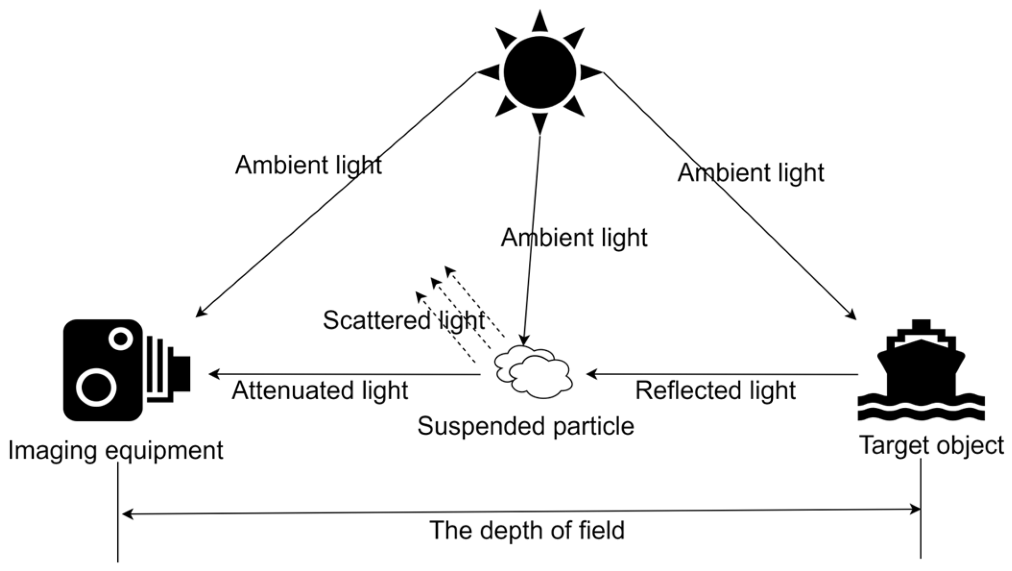
Physical model-based methods can analyze image information according to the mathematical model of foggy imaging [13], and they can use prior knowledge to obtain the dehazed image. As shown in Figure 1, the model is mainly based on the scattering and absorption of light in atmospheric media and simulates the image degradation phenomenon that occurs under complex atmospheric conditions. Therefore, researchers have proposed several methods to estimate the correlation coefficient for calculating the defogged image. Among these, the dark channel prior method proposed by He et al. [14] is one of the most common algorithms. Due to the large sky areas and high white light components, it is easy to obtain higher values in all three channels using this method. Therefore, researchers have proposed a series of improved algorithms based on the dark channel prior method. Zhao et al. [15] proposed segmenting the image using the four-division method to select the best area for the estimation of atmospheric light value, aiming to address the problem of color spots in the sky area during the processing of the original dark channel prior theory. Zhou et al. [16] proposed segmenting the sky region based on the gray feature value to better calculate the atmospheric light value. In the bright channel prior theory, it is assumed that at least one color channel pixel in certain target areas has a reflectance of 100%, allowing for better differentiation of images in large sky backgrounds using this theory. Liu et al. [17] proposed using the L channel of the Lab color space as a guide map, predicting the atmospheric light value through guided filtering, and then estimating the transmittance by using the bright channel prior theory. Zhang et al. [18] proposed using the Al-Alaoui operator to enhance the image through convolution filtering, and based on this, to carry out dehazing. Combining the two theories to process different image regions separately is also common. Yu et al. [19] proposed a pixel-wise alpha blending method for estimating the transmission map, where the transmissions estimated from the dark channel prior and the proposed bright channel prior are effectively blended into one transmission map, guided by a brightness-aware weights map. Tang et al. [20] combined and corrected the two estimation methods of transmittance by assigning different weights. These methods, which study the imaging principle of the object, have a significantly better dehazing effect than image enhancement-based methods. However, a priori assumptions need to be utilized for the evaluation of transmittance and global atmospheric light. These assumptions will fail in certain situations, such as image distortion when processing large sky areas.

Figure 1. The light reflected from the surface of the target object is absorbed and scattered by the suspended particles in the atmospheric medium during propagation, resulting in light attenuation. Ambient light scatters in the atmospheric medium, which affects the brightness distribution of the imaging. Through the superposition effect of these two physical processes, the final imaging exhibits problems such as contrast drop and color distortion.

Deep learning-based methods can use a large amount of data to learn the mapping relationships between haze-free images. Cai et al. proposed the DehazeNet network [21] to estimate transmittance and atmospheric light values and perform dehazing of images based on the atmospheric scattering model. Li et al. first proposed the end-to-end dehazing network, AOD-Net [22]. To address the problem of grid artifacts easily caused by dilated convolution, Chen et al. proposed an end-to-end gated context aggregation network, GCA-Net [23]. Li et al. proposed an image dehazing network with an encoding and decoding structure based on a conditional generative adversarial network (GAN) [24]. Engin et al. proposed Cycle-Dehaze [25], combining cyclic consistency loss and perceptual loss to train the network. Zhao et al. proposed an encoder–decoder based on GAN [26] to further improve the network dehazing capability by learning different high- and low-frequency information of the image. Hyun Kwon proposed a novel method for generating untargeted adversarial examples using GAN in an unrestricted black box environment [27]. Song et al. proposed DehazeFormer for image dehazing, based on the Transformer model [28]. These methods have achieved significant results by leveraging the learning capability of neural networks. However, they heavily depend on extensive natural scene datasets, and it is easy to overfit during the learning process, resulting in a general effect in real scene dehazing.

In conclusion, although image enhancement-based methods are simple, they can easily lose image detail information and exhibit poor robustness. Physical model-based methods can analyze the reasons for image degradation, but in practical applications, they can suffer from parameter estimation biases, which lead to incomplete image dehazing. Deep learning-based methods can learn from a large amount of image data, understand image information more accurately, and exhibit strong adaptability. Therefore, we choose deep learning-based methods for multi-scene image dehazing. However, this type of method requires a large amount of data for training. It is difficult to obtain paired datasets, and using synthetic datasets can easily lead to overfitting. Additionally, problems such as insufficient use of feature information can result in blurred edges and loss of fine details in dehazed images. To address these issues, we propose an improved model of cyclic generative adversarial networks. The network is based on CycleGAN for image dehazing, using unpaired datasets for model training, which can alleviate the overfitting problem to some extent. A weight allocation mechanism is introduced into feature fusion to make full use of feature information and retain image details after dehazing.

3. Methods

Since paired haze-free datasets are difficult to obtain in many scenarios, the extensive use of synthetic datasets may lead to overfitting issues in deep learning models, resulting in insignificant dehazing effects in real-world images. Using the CycleGAN unpaired image-to-image translation framework, the image dehazing problem is treated as an image transformation between two distinct style domains. Hazy images are considered the source domain, while haze-free images are regarded as the target domain. The core of the CycleGAN-based image dehazing method lies in mapping the source domain images to the target domain, transforming haze images into haze-free images. However, the physical properties of hazy environments in the real world are often ignored in end-to-end dehazing methods, resulting in generated haze that usually lacks realism and diversity, further impacting the learning of the subsequent dehazing network. To address the abovementioned issues, we propose the FA-CycleGAN model. Using the CycleGAN model can effectively solve the problem of difficult pairwise image acquisition. In the training process, convolutional operations are used to extract the parameters of the atmospheric scattering model and reconstruct the clear image. At the same time, a deep learning model is used to refine the process to make up for the parameter estimation error of the atmospheric scattering model. A feature fusion attention module is introduced into the generator structure for multi-scale feature fusion and different weight assignments, which can retain more feature information and focus on different regions’ features to varying degrees. While ensuring the authenticity of dehazed images, more image details are retained, and the dehazing performance of the model is improved.

3.1. Overall Framework of the Model

In this paper, the atmospheric scattering model is used as a physical constraint in combination with CycleGAN. On the theoretical basis of the mathematical model, the hazy imaging atmospheric scattering model can be described as follows:

$$H(x)=C(x)t(x)+A(1-t(x))$$

(1)

where H(x) is the X-th pixel value of the hazy image, C(x) is the dehazed image, A is the global atmospheric light value, and t(x) is the transmittance. The relationship between the transmittance and the depth information of the image is shown in Equation (2), where β is the scattering coefficient and d(x) is the depth information of the image.

$$t(x)=e^{-\beta d(x)}$$

(2)

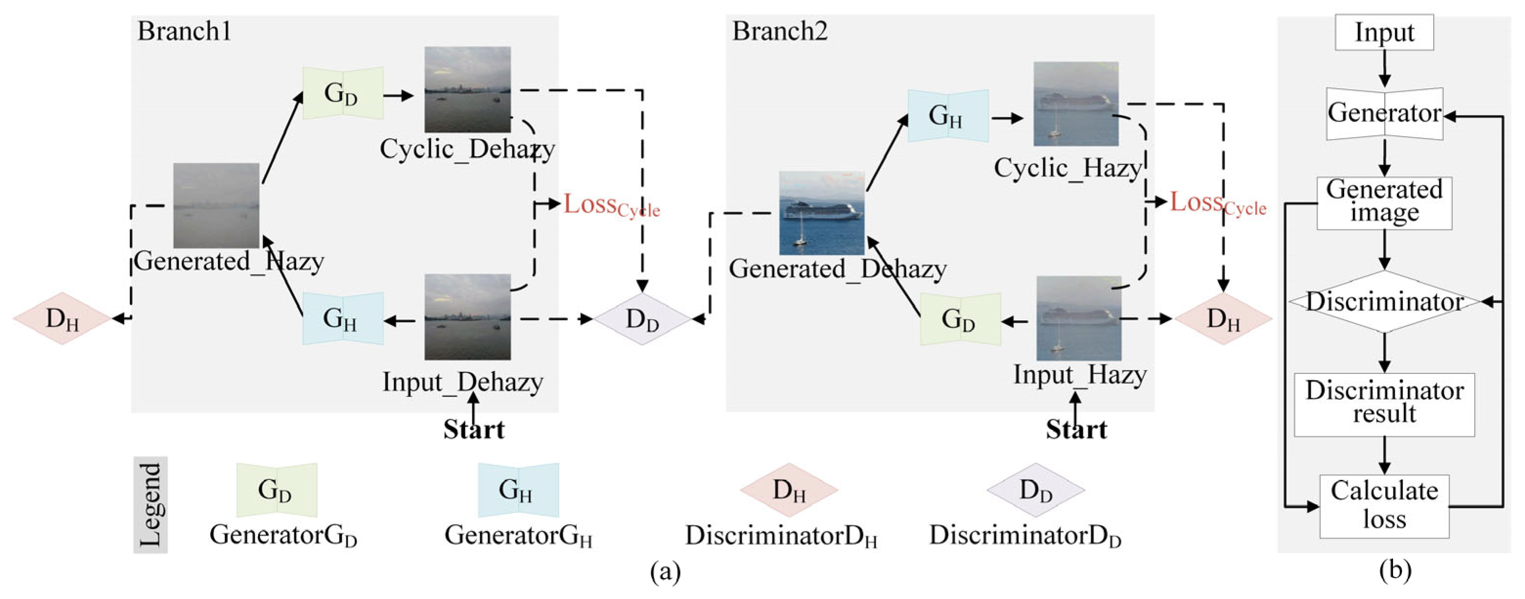
Based on the improvements to the CycleGAN network, FA-CycleGAN is proposed. Its structure is shown in Figure 2a. FA-CycleGAN consists of two generators and two discriminators. Haze-free images are generated from haze images by the generator, G_D, aligning their distribution with that of the target domain images, thereby deceiving the discriminator D_D. Haze images are generated from haze-free images by the generator, G_H, to deceive the discriminator, D_H. The discriminator, D_H, is responsible for determining whether the input image is a haze image, while the discriminator, D_D, assesses whether the input image is a haze-free image.

Figure 2. The proposed FA-CycleGAN consists of two generators and two discriminators, and the two branches of the network are used to generate hazy and haze-free images as shown as (a). The workflow of generator G_D and generator G_H is shown in (b).

The workflow of generator G_D and generator G_H is shown in Figure 2b. The image is fed into the generator to produce the generated image. This generated image is then fed into the discriminator to determine whether it is a real image. Then, the loss is calculated based on the generated image and the discriminator’s results, followed by updating the generator and discriminator parameters based on this loss. During the training process, increasingly realistic images are produced by the generator in an attempt to deceive the discriminator, which is used to distinguish between real and generated images. Through the adversarial interaction between the generator and discriminator, the conversion of haze images to haze-free images is achieved. Finally, an optimal paired image generator model with haze and haze-free images is obtained. The pseudocode is as shown in Algorithm 1.

Algorithm 1 FA-CycleGAN Network Training Process

Input: Input_Dehazy, Input_Hazy.//clear images and hazy images.

Output: Training log information.

1: #===== Branch1: Clean → Hazy → Cyclic Clean ===== 2: Generated_Hazy, gt_beta = GH(Input_Dehazy) 3: Cyclic_Dehazy, pred_beta = GD(Generated_Hazy) 4: # ===== Branch2: Hazy → Dehazy → Cyclic Hazy ===== 5: Generated_Dehazy, gt_d = GD(Input_Hazy) 6: Cyclic_Hazy, pred_d = GH(Generated_Dehazy) 7: # ===== Discriminators training ===== 8: dis_real_clean = DD(Input_Dehazy) 9: dis_fake_clean = DD(Generated_Dehazy) 10: loss_dis_clean = adversarial_loss(dis_real_clean, True) + adversarial_loss(dis_fake_clean, False) 11: dis_real_hazy = DH(Input_Hazy) 12: dis_fake_hazy = DH(Generated_Hazy) 13: loss_dis_hazy = adversarial_loss(dis_real_hazy, True) + adversarial_loss(dis_fake_hazy, False) 14: total_dis_loss = (loss_dis_clean + loss_dis_hazy)/4 15: total_dis_loss.backward() 16: # ===== Generators training ===== 17: fake_clean_logits = DH(Generated_Dehazy) 18: fake_hazy_logits = DD(Generated_Hazy) 19: loss_gan = (adversarial_loss(fake_clean_logits, True) + adversarial_loss(fake_hazy_logits, True))/2 20: loss_cycle = L1(Input_Hazy, Cyclic_Hazy) + L1(Input_Dehazy, Cyclic_Dehazy) 21: loss_β = L2(pred_beta, gt_beta) 22: loss_d = L1(gt_d, pred_d) 23: total_gen_loss = λ_gen*loss_gan + λ_cycle*loss_cycle + λ_β*loss_β + λ_d*loss_d 24: total_gen_loss.backward()

3.2. Structure of the Specific Network

3.2.1. Structure of the Generators

Unlike traditional CycleGAN, a heterogeneous generator structure, in which the two generators utilize different network structures, is employed in FA-CycleGAN.

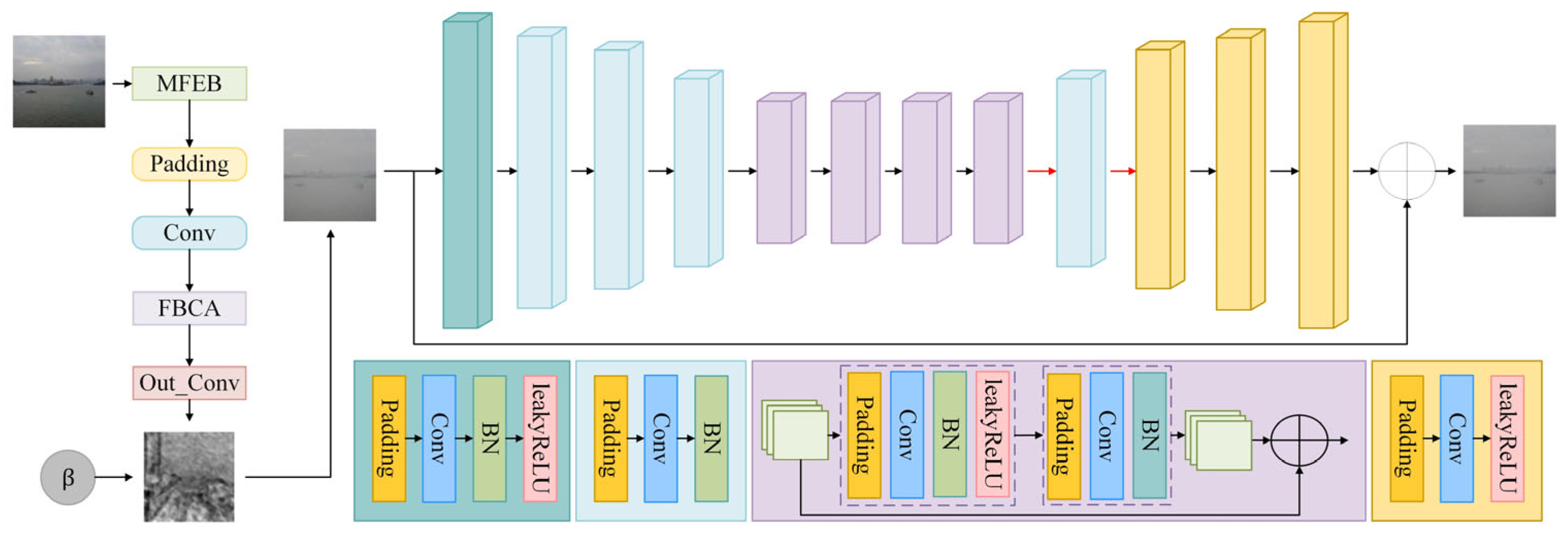
Image dehazing is performed on the input hazy image by the G_D. The model structure is shown in Figure 3. The pseudocode is shown in Algorithm 2. The depth information of the image is estimated through feature extraction and residual fusion by the transmittance estimation module. The scattering coefficient of the image is estimated through feature extraction and average pooling operations by the scattering coefficient estimation module. G_D is first used to extract features from the input image, H. The extracted features at different levels are processed to obtain the image’s transmittance, $\widehat{t}$, and scattering coefficient, $\widehat{\beta }$, as follows:

$$(\widehat{t},\widehat{\beta })={\mathrm{G}}_{\mathrm{D}}(H)$$

(3)

Figure 3. The transmittance and scattering coefficients are estimated through the generator G_D using feature extraction and fusion, and a haze-free image is obtained by calculating Equation (4).

The generated haze-free image, $\widehat{C}$, can be calculated based on the atmospheric scattering model as follows:

$$\widehat{C}={\displaystyle \frac{H-\widehat{A}}{\widehat{t}}}+\widehat{A}$$

(4)

where $\widehat{A}$ is the atmospheric light value estimated from the dark channel prior, H is the hazy images, and $\widehat{t}$ is the image’s transmittance.

Algorithm 2 Process flow of the generator, GD

Input: Input_Hazy.//hazy images.

Output: Generated_Dehazy.

1: Initialize: 2:    Bulid the multi-layer feature extraction block(MFEB) 3:    Build the feature fusion attention block(FBCA) 4:    Build the output layers(output_Conv) 5: Method forward_get_A(input_image) 6:    If use_dc_A 7:        then Estimate atmospheric light A via dark channel method 8:        else Set A as the maximum RGB value over spatial dimensions 9:    return A 10: Method forward(Input_Hazy) 11:    features = MFEB(Input_Hazy) 12:    t = output_Conv(FBCA(features)) 13:    β = AvgPooling(features) 14:    Normalize t and β into valid ranges 15:    A = forward_get_A(Input_Hazy) 16:    Compute Generated_Dehazy according to Equation (4)

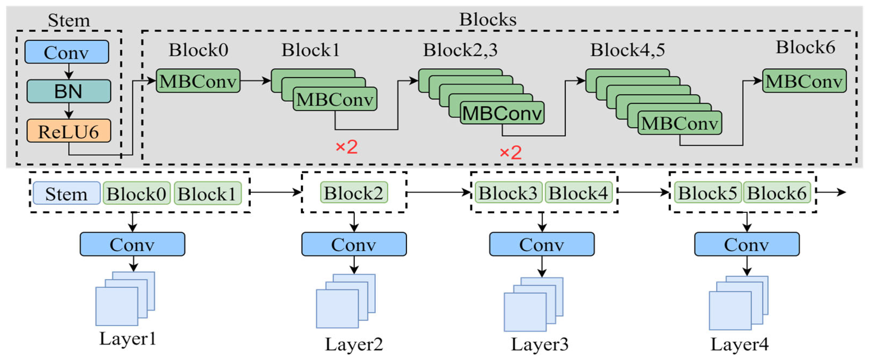
As shown in Figure 4, the multi-layer feature extraction block (MFEB) is built based on the EfficientNet-lite3 network. The backbone network is divided into four layers to gradually extract advanced features from the image. Through layered feature extraction, the network can gradually learn low-level details and high-level semantic information, which aids in learning complex structures and patterns in the image, enabling the network to better understand the input data.

Figure 4. The multi-layer feature extraction block can extract features using multiple MBConv structures and output multi-layer features.

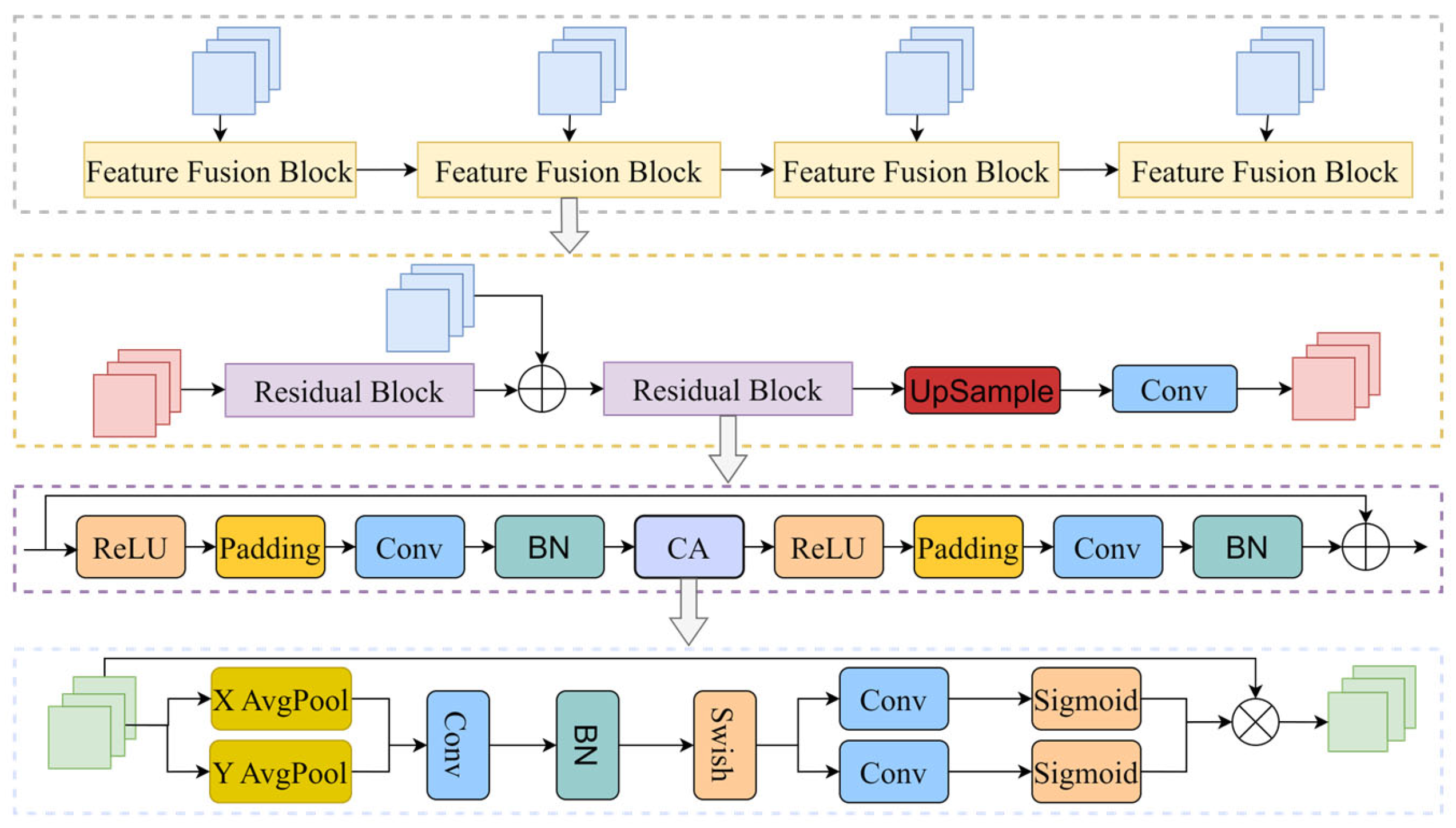
The feature fusion attention module (FBCA) performs multi-scale feature fusion on extracted features of different levels. Its structure is shown in Figure 5. The idea of residual connection is adopted in FBCA, where different levels of features are separately fed into different feature fusion blocks for fusion. The output of the previous layer’s feature fusion block is processed by a residual unit and added to the input features of the current layer. The result of this addition is then processed by the residual unit to obtain the output of the current layer. This approach allows for improved retention of low-level features while promoting the learning of high-level features, thus improving the dehazing effect. To enhance the model’s attention to input data, the CA attention module is introduced to improve the model’s performance in handling complex tasks. In this module, the model can focus on complex areas to recover details more efficiently. Most current attention mechanisms (e.g., SE attention mechanism) significantly enhance model performance. Unlike traditional channel attention, which aggregates spatial information globally and may overlook location-specific features, attention is decomposed by CA into two complementary 1D encodings along the horizontal and vertical directions. This approach captures long-range dependencies while preserving precise positional information. By embedding location awareness into channel attention, CA allows the network to adaptively emphasize features that are not only important across channels but also relevant to specific spatial coordinates. This enables the generator to identify and enhance important regions, such as object boundaries, edges, and textured areas, which are often degraded or obscured in hazy images. This results in better structural preservation, reduced artifacts, and improved clarity in localized areas in practice. Thus, the integration of CA within the FBCA module helps the network focus on both channel importance and spatial position, leading to a more refined feature representation that contributes to more effective and visually coherent dehazing outcomes.

Figure 5. The feature fusion attention block can accept the multi-layer features extracted by the MFEB and feed them into different feature fusion blocks for fusion. The feature fusion block is described in the second box, and the residual block is described in the third box.

Image hazing is performed by the G_H based on the input clear image. The model structure is shown in Figure 6. The pseudocode is shown in Algorithm 3. Firstly, the transmittance estimation module is used to estimate the depth information, $\widehat{d}$, of the input clear image, and a scattering coefficient, β, is randomly sampled within the range of [0.6, 1.8]. Then, the atmospheric scattering model is used to calculate a rough pseudo-hazy image. Finally, the rough pseudo-hazy image is refined using the U-Net network to avoid the visual unreality of the image caused by parameter estimation errors, as follows:

$$\widehat{H}={\mathrm{G}}_{\mathrm{H}}(C{e}^{-\beta \widehat{d}}+A(1-e^{-\beta \widehat{d}}))$$

(5)

Algorithm 3 Process flow of the generator, GH

Input: Input_Dehazy.//clear images.

Output: Generated_Hazy.

17: Initialize: 18:    Bulid the multi-layer feature extraction block(MFEB) 19:    Build the feature fusion attention block(FBCA) 20:    Build the output layers(output_Conv) 21:    Build the U-Net network(UNet) 22: Method forward(Input_Dehazy) 23:    features = MFEB(Input_Dehazy) 24:    d = output_Conv(FBCA(Conv(features))) 25:    β = Ramdom [0.8, 1.6] 26:    Compute Generated_Hazy according to Eqs.(5) 27:    Generated_Hazy = UNet(Generated_Hazy)//Refined by U-Net

Figure 6. The generator, G_H, can estimate the depth information of the image through feature extraction and fusion and combine the randomly generated scattering system to obtain a rough blurred image, as calculated using Equation (5). Finally, it uses the U-Net network for fine processing to obtain the final haze image.

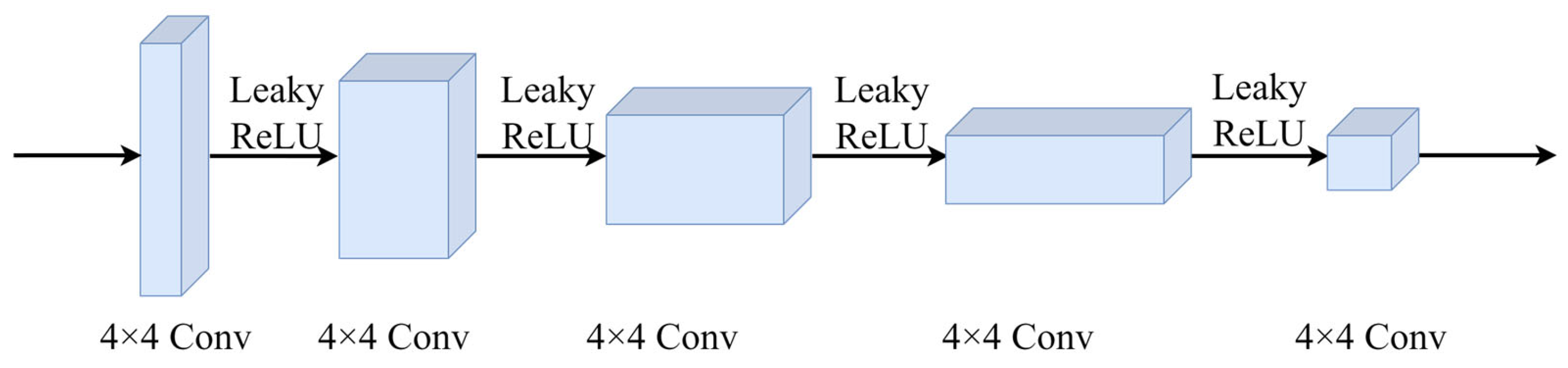
3.2.2. Structure of the Discriminator

A basic convolutional discriminator was used to distinguish between real and generated images. Its network structure is shown in Figure 7. The discriminator receives the input image and performs feature extraction through a series of convolutional operations. Spectral normalization is applied to stabilize the training process. Using LeakyReLU as the activation function helps preserve more information and prevent gradient vanishing issues. The last layer maps the output to the range [0, 1], providing the probability that the input image is a real image.

Figure 7. The discriminator can output the final discrimination result through a layer-by-layer convolution structure.

3.3. Loss Function

Similar to CycleGAN, cyclic consistency loss and adversarial training loss are used to penalize content consistency and data distribution, respectively. According to the atmospheric scattering model, the degree of fog in the real world is related to the scene depth, d, and the scattering coefficient, β. Therefore, pseudo scattering coefficient-supervised loss and pseudo depth-supervised loss are employed to learn physical properties (depth and density) from unpaired hazy-free images.

Adversarial training loss is used to evaluate whether the generated images belong to a specific domain, penalizing the visual fidelity of the hazy and free images while ensuring that they follow the same distribution as the images in the training set. To address the issue of slow convergence of the discriminator caused by the min–max loss, non-saturating GAN (NSGAN) [29] loss is used. NSGAN loss has good stability and visual quality. For the generator, G, and the corresponding discriminator, D, the adversarial loss can be expressed as follows, where rh is real_hazy sample of the hazy image set, and rc is real_clean sample of the clean image set:

$$Los{s}_{\mathrm{GAN}}({\mathrm{G}}_{\mathrm{H}},{\mathrm{D}}_{\mathrm{H}})=\mathrm{E}[\log ({\mathrm{D}}_{\mathrm{H}}(rh)]+\mathrm{E}[\log (1-{\mathrm{D}}_{\mathrm{H}}({\mathrm{G}}_{\mathrm{H}}(rc))]$$

(6)

$$Los{s}_{\mathrm{GAN}}({\mathrm{G}}_{\mathrm{D}},{\mathrm{D}}_{\mathrm{D}})=\mathrm{E}[\log ({\mathrm{D}}_{\mathrm{D}}(r\mathrm{c})]+\mathrm{E}[\log (1-{\mathrm{D}}_{\mathrm{D}}({\mathrm{G}}_{\mathrm{D}}(rh))]$$

(7)

Training CycleGAN using only adversarial training loss does not guarantee the cyclic consistency of the network [30], which refers to the consistency between the input and output. Therefore, cyclic consistency loss is used to penalize the consistency of the inputs and outputs. This loss is defined as the difference between the input value, x, and the forward prediction, F(G(x)), as well as the input value, y, and the forward prediction, G(F(y)). The larger the difference, the further the prediction is from the original input. The cyclic consistency loss is implemented using L1 loss, as shown in Equation (8) as follows:

$$Los{s}_{\mathrm{cycle}}=\mathrm{E}[{\mathrm{G}}_{\mathrm{H}}({\mathrm{G}}_{\mathrm{D}}(rh))-rh]+\mathrm{E}[{\mathrm{G}}_{\mathrm{D}}({\mathrm{G}}_{\mathrm{H}}(rc))-rc]$$

(8)

The pseudo-scattering coefficient supervised loss is used to penalize the difference between the randomly sampled scattering coefficients generated and the scattering coefficients estimated from the generated hazy images. It is calculated as follows:

$$Los{s}_{\mathsf{\beta }}={(\widehat{\beta }-\beta )}^2$$

(9)

Pseudo-depth supervised loss is used to penalize the difference between the depth information, d, estimated from the hazy image, H, and the depth information, $\widehat{d}$, estimated from the dehazed image. The L1 loss is used, which is defined as follows:

$$Los{s}_{\mathrm{d}}=\mathrm{E}[\widehat{d}-d]$$

(10)

In summary, joint optimization is performed using a weighted combination of the abovementioned losses as follows:

$$Los{s}_{\mathrm{total}}={\lambda }_{\mathrm{GAN}}Los{s}_{\mathrm{GAN}}+{\lambda }_{\mathrm{cycle}}Los{s}_{\mathrm{cycle}}+{\lambda }_{\mathsf{\beta }}Los{s}_{\mathsf{\beta }}+{\lambda }_{\mathrm{d}}Los{s}_{\mathrm{d}}$$

(11)

where λ_GAN, λ_cycle, λ_β, and λ_d are the weights used to balance different items. Based on previous experience and experiments conducted, setting these weights to 0.2, 1, 1, and 1, respectively, works well in our experiments.

4. Experiment

4.1. Experimental Environment and Parameters

In this paper, we use Python 3.9 and PyTorch 1.12 to build a deep learning environment and conduct experiments on an NVIDIA GeForce RTX 3060 Laptop GPU. The network is trained using the RGB channel. The training images are cropped to 256 × 256 as the input for the network. The model is trained using the Adam Optimizer, where the batch size is set to 2, the average gradient values β₁ and β₂ are set to 0.9 and 0.999, respectively, and the learning rate is set to 0.0001.

4.2. Datasets and Evaluation Indicators

4.2.1. Datasets

The public datasets used for evaluating the model in this paper mainly include the RESIDE dataset and the I-HAZE dataset. RESIDE is a large synthetic dataset divided into five subsets. We selected the Outdoor Training Set (OTS) and the Synthetic Outdoor Testing Set (SOTS) for experimentation. OTS contains 2061 clear outdoor images and 72,135 hazy images. Each clear image corresponds to 35 blurred images with different atmospheric light values and scattering coefficients. SOTS contains 500 indoor clear images and 500 clear outdoor images, along with their corresponding hazy images. The I-HAZE dataset is used to evaluate the performance of the algorithm in a real hazy environment, using an artificial fog device to generate real fog in an indoor setting.

Currently, there are many indoor and outdoor hazy image datasets based on land, covering different scene types. However, there are hardly any publicly available datasets specifically for maritime hazy images. To address this issue, we used a hazing algorithm to fog natural images and constructed a maritime dehazing dataset called the Maritime Dehaze Dataset (MDD). To prevent overfitting, we collected maritime images from different scenes. Various visual scenes in the maritime domain are covered comprehensively in MDD, including inland waterway shipping, ports, near-shore coastal areas, watercraft, and buoy small target detection. In the MDD, there are a total of 2142 images for training and 200 for testing.

4.2.2. Evaluation Indicators

In order to evaluate the advantages and disadvantages of the algorithm objectively, a variety of indexes are used. The first is the full reference evaluation index: structural similarity (SSIM) and peak signal-to-noise ratio (PSNR). The structural similarity index between two images can be compared using SSIM, which is based on the mean, variance, and covariance of the images. PSNR is a measure of the relationship between signal and noise and is used to evaluate the quality of image reconstruction. This is followed by no-reference evaluation indicators: information entropy (IE) and Natural Image Quality Evaluation Index (NIQE). IE is an important index for measuring image complexity and information, which is used to evaluate image detail and contrast after fog removal. The quality of an image can be evaluated using the NIQE by analyzing its structural and statistical characteristics and comparing them with the typical features of a natural image, which helps assess whether an image appears visually natural. Finally, there are performance metrics: number of parameters (Params) and floating point operations per second (FLOPs). These two key metrics are used to evaluate the performance and efficiency of the model and are used to measure the complexity and computational requirements of the improved model.

4.3. Comparative Experiments

To validate the effectiveness of the algorithm, we compared it with several classical and advanced dehazing methods, including DCP, CycleDehaze, FFANet, MSBDN, C2PNet, and our method. DCP is a classic prior knowledge-based method. CycleDehaze is an improved algorithm based on CycleGAN. A new feature fusion attention module is proposed with FFANet, which combines channel attention and pixel attention for feature weighting. A multi-scale dense feature fusion module is proposed with MSBDN, which is based on combining U-Net with the back-projection feedback scheme in image super-resolution. A physical-aware dual-branch unit is proposed with C2PNet, which assigns the estimation tasks of transmittance and atmospheric light value to two parallel branches for learning based on the atmospheric scattering model. To qualitatively compare the strengths and weaknesses of these algorithms, a unified dataset and training scheme are used to train the networks.

4.3.1. Land Scene

In the land scene, the OTS is used for training models and comparison methods. SOTS-outdoor was synthesized in the same way as OTS and was selected as one of the test sets. SOTS-indoor and I-HAZE differ in terms of scenes and haze types, and the results from these two test sets can reflect the adaptability of the model to different scenes. The comparison results are shown in Table 1. The visualization results are shown in Figure 8.

Table 1. Comparison results of different models using the SOTS-outdoor, SOTS-indoor, and I-HAZE datasets.

Metrics		SOTS-Outdoor		SOTS-Indoor		I-HAZE
Method		PSNR	SSIM	PSNR	SSIM	PSNR	SSIM
paired	(a) FFANet	36.361	0.993	20.230	0.855	16.437	0.747
	(b) C2PNet	36.180	0.989	21.213	0.897	16.650	0.733
	(c) MSBDN	33.794	0.983	21.330	0.837	16.056	0.769
unpaired	(d) DCP	18.158	0.804	18.640	0.792	14.444	0.629
	(e) Cycle-Dehaze	15.835	0.789	11.961	0.688	14.318	0.605
	(f) Ours	26.248	0.945	22.385	0.903	16.681	0.816

Figure 8. (Hazy) and (Clear) are the land images of SOTS-outdoor dataset, and (a–f) are the dehazing experimental results of method FFANet, C2PNet, MSBDN, DCP, Cycledehaze, and the proposed method.

In the experimental comparisons using the SOTS-outdoor dataset as the test set, strong fitting capabilities were demonstrated in the supervised FFANet due to the consistency between SOTS-outdoor and the training set OTS in synthetic methods. The best results were achieved using our method among those trained on non-paired datasets. Under unsupervised conditions, image features can be learned effectively by the method, leading to high-quality predictions and demonstrating its potential and advantages in the absence of paired data. In the experimental comparisons using the SOTS-indoor and I-HAZE datasets as the test sets, due to the inconsistency between the test sets and OTS in synthetic methods, the supervised model failed to adapt effectively to changes in the data distribution. In this case, the advantages of supervised methods are significantly diminished, and there is even a slight overfitting phenomenon, leading to a decline in performance on both datasets. In contrast, our proposed method exhibits stable performance on both datasets. In the two image quality evaluation indices of SSIM and PSNR, compared with other existing comparison methods, the proposed method shows better adaptability across diverse datasets. Based on the experimental results, it can be observed that the proposed method not only overcomes the adverse effects caused by the inconsistency of synthetic datasets but also maintains relatively consistent performance across different test sets. This further verifies its effectiveness and feasibility within unsupervised learning.

As can be seen in the visualization results in Figure 8d, DCP is a classic prior-based method that relies on the dark channel prior derived from the atmospheric scattering model. However, it struggles to adapt to complex scenes and often leads to color distortions or over-dehazing. C2PNet, shown in Figure 8b, explicitly incorporates the atmospheric scattering model by proposing a physical-aware dual-branch unit, which assigns the estimation of transmittance and atmospheric light to two separate learning branches. This design significantly improves the accuracy of key parameter estimation, thus enhancing the model’s robustness. On the other hand, cycle consistency constraints for unsupervised learning is introduced by CycleDehaze, but explicit modeling of the physical scattering process is lacking, resulting in weaker performance in physical consistency and detail restoration, as shown in Figure 8e. A feature fusion attention module is introduced by FFANet to adaptively weight features at different scales and regions, as shown in Figure 8a. This significantly enhances the representation capacity of dehazing features and improves the fidelity of image restoration. While not employing an explicit attention mechanism, effective cross-scale feature fusion is achieved by MSBDN through dense connections and feature feedback, which improves dehazing performance to a considerable extent, as shown in Figure 8c. However, when there is a large sky area and strong illumination, most methods encounter problems of incomplete dehazing and distortion in the sky area. The atmospheric scattering model is combined with the CycleGAN network in the proposed method, which can correct parameter estimation errors while retaining physical information. At the same time, the feature fusion attention mechanism is introduced, which can retain feature information to the greatest extent, sro that more details can be retained and the problem of color distortion can be corrected. Therefore, the restored image is closer to the visual effect of a real image.

4.3.2. Maritime Scene

In this section, experiments are conducted using the MDD for training and testing. The results are compared with current classical and more cutting-edge dehazing algorithms. The comparison results are shown in Table 2. The visualization results are shown in Figure 9.

Table 2. Comparison results of different models using MDD.

	Paired			Unpaired
	(a) FFANet	(b) C2PNet	(c) MSBDN	(d) DCP	(e) CycleDehaze	(f) Ours
PSNR↑	16.437	19.061	13.296	15.497	13.196	24.850
SSIM↑	0.747	0.862	0.423	0.744	0.730	0.956
IE↑	6.997	7.278	7.271	6.895	6.564	7.433
NIQE↓	2.522	2.491	2.543	2.580	2.557	2.431

Figure 9. (Hazy) and (Clear) are the maritime images of MDD dataset, and (a–f) are the dehazing experimental results of method FFANet, C2PNet, MSBDN, DCP, Cycledehaze, and the proposed method.

In Table 2, it can be seen that our proposed network has relatively stable performance on MDD. The SSIM and PSNR values were 24.850 and 0.956, both achieving the highest scores. The PSNR and SSIM values can reflect the similarity between the dehazed image and the real image. The FBCA weighting mechanism proposed in this paper assigns higher weights to important features, retaining details while suppressing useless noise. Image structure information and details can be recovered better, thereby improving the PSNR and SSIM indicators. Information entropy reflects image complexity and information content. The maximum value of 7.433 is obtained in IE, indicating that the image, after using the model to remove fog, is clearer and more detailed. This improvement is due to the introduction of multi-scale feature fusion and a weighting mechanism in the model, which allows the model to effectively capture high-frequency information, thereby improving the clarity and information of the image. The NIQE index evaluates whether the image is visually natural. The optimal value of the NIQE index indicates that the defogged image has recovered details and textures and is more in line with human visual perception.

The visualization results are shown in Figure 9. MSBDN and CycleDehaze exhibited poor performance on the MDD dataset, resulting in a significant amount of haze residue in the dehazed images and incomplete dehazing, which indicates that their modeling ability for maritime scenes is insufficient because they cannot effectively distinguish between haze and image information. Since DCP is based on the dark channel prior method, it is prone to large-area color distortion in bright areas such as the sky, and there is a degree of image over-exposure. The two networks, FFANet and C2PNet, perform relatively well, but there is some color distortion because the feature differences of different regions are not fully considered in the fusion process of feature extraction. In contrast, the deep learning model is used in the proposed method to extract the parameters of the atmospheric scattering model and refine them. At the same time, a multi-scale feature fusion and weighting strategy is introduced. This model can capture both global and local features and dynamically adjust the weights so as to maintain high dehazing performance in complex scenes, and the visual effect in the dehazed images is more natural.

4.4. Ablation Experiments

4.4.1. Comparison of Different Modules

To further verify the effectiveness of each module in the network, ablation experiments were designed with different model states. The results of the module effectiveness experiments are shown in Table 3, and the visualization results are shown in Figure 9. In the table, the base model is the CycleGAN; “A” is the improved generator structure based on the atmospheric scattering model, “B” is the improved loss function, and “C” is the FBCA module in the network. The comparison results are shown in Table 3. The visualization results are shown in Figure 10.

Table 3. Objective comparison of ablation results of different modules.

A	B	C	PSNR↑	SSIM↑	IE↑	NIQE↓	Params (M)↓	FLOPs (GMac)↓
×	×	×	19.870	0.721	7.093	3.045	11.381	45.571
√	×	×	23.069	0.903	7.115	2.912	10.697	2.246
√	√	×	24.702	0.915	7.362	2.537	10.697	2.246
√	×	√	25.243	0.926	7.414	2.580	10.757	2.311
	√	√	26.248	0.945	7.433	2.431	10.757	2.311

Figure 10. Comparison of PSNR and generator loss metrics compared to the baseline model during training.

As shown in Table 3, by improving the generator network structure, the PSNR and SSIM increase by 16.10% and 25.24%, respectively, indicating that after combining the atmospheric scattering model, the model can make full use of the physical characteristics of fog to better learn image features. The generator of the traditional CycleGAN is based on a residual network, which is more complex to calculate, while the improved generator greatly reduces the amount of computation, thus achieving better results in terms of FLOPs. After the introduction of the improved loss function, the performance of the model is further improved, indicating that the optimization of the loss function can better guide model training and optimize parameters. Compared with the original network, the PSNR increases by 32.10%, the SSIM increases by 31.07%, the information entropy increases by 4.79%, and the NIQE index is reduced by 20.1%, indicating that the quality of the dehazed image has been significantly improved. With the introduction of the FBCA module, the best test results were achieved, with a 32.10% increase in PSNR and a 31.07% increase in SSIM compared to the original network. The dehazed image processed by the model is clearer and more in line with human visual perception. Due to the introduction of the FBCA module, the proposed method results in a moderate increase in the indicators of Params and FLOPs. However, as demonstrated by the experimental results, this increase leads to significant improvements in performance, representing a reasonable trade-off between performance and computational cost. As shown in Figure 10a, it can be observed that with the increase in training epochs, the PSNR of both methods shows an overall upward trend. However, FA-CycleGAN consistently achieves higher PSNR values across different stages and exhibits smaller fluctuations, indicating better stability and convergence. These results demonstrate that FA-CycleGAN is capable of generating higher-quality dehazed images, thereby validating the effectiveness of the proposed method in preserving image details and improving dehazing performance. As shown in Figure 10b, both models exhibit a decreasing trend in loss as training progresses, indicating successful convergence. Notably, FA-CycleGAN maintains consistently lower loss values with smaller fluctuations throughout the training process and converges more rapidly compared to CycleGAN. This result further supports the effectiveness of FA-CycleGAN in achieving better stability and optimization during model training.

From the visual effects shown in Figure 11, it can be observed that the original CycleGAN network’s dehazing is not thorough, with “pseudo-shadows” present in some areas and the sky area exhibiting localized exposure. After improving the generators based on the atmospheric scattering model and loss function, the model can make full use of physical prior information; there are no longer any “artifacts”, and the local exposure of the sky area is improved. This demonstrates that physical prior modeling effectively provides more reasonable guidance for dehazing. After introducing the FBCA module, the model can fully integrate the features of each level and assign different weights. The model exhibited significantly enhanced restoration capabilities in detailed regions (such as object edges and texture-rich areas). Therefore, the model can effectively restore image color, dehazes more thoroughly, and significantly improves the visual effect. On the whole, the ablation experimental results fully verify the effectiveness of each improved module, achieving the best performance across multiple evaluation indicators. The improved model enhances the understanding and generation ability of image information, which helps further improve the dehazing performance of the model, so that the processed image can retain more details and generate images that are more in line with human eye perception.

Figure 11. (Hazy) and (Clear) are the images of SOTS-outdoor dataset, and (a–e) are the visualization results of different ablation modules.

4.4.2. Comparison of Different Attention Mechanisms

In this section, ablation experiments on different attention mechanisms in the FBCA module were conducted. The impact of these attention mechanisms on model performance is evaluated through comparison. The OTS dataset is used as the training set, and the SOTS-outdoor dataset is used as the validation set to verify the effectiveness of the selected mechanisms. Specifically, the FBCA module without attention mechanisms is labeled as “None”. The names of the introduced attention mechanisms are used as module names, including the channel attention mechanism, Convolutional Block Attention Module (CBAM) mechanism, ShuffleAttention mechanism, SKAttention mechanism, and CA mechanism used in this paper. The quantitative evaluation results are shown in Table 4, and the visual results are shown in Figure 12.

Table 4. Objective comparison results of different attention mechanisms.

	(a) None	(b) Channel Attention	(c) CBAM	(d) ShuffleAttention	(e) SK Attention	(f) Ours
PSNR↑	23.069	22.091	25.679	25.358	24.819	26.248
SSIM↑	0.903	0.879	0.930	0.921	0.918	0.945
IE↑	7.115	7.219	7.373	7.362	7.296	7.433
NIQE↓	2.879	2.697	2.491	2.524	2.452	2.431

Figure 12. (Hazy) and (Clear) are the images of SOTS-outdoor dataset, (a) is the dehazing result without introducing the attention mechanism, and (b–f) are the dehazing results of attention mechanism channel attention, CBAM, shuffle attention, SK attention and ours.

In Table 4, it can be seen that when only the channel attention mechanism is used, the PSNR, SSIM, and IE metrics decreased by 4.24%, 2.66%, and 6.32%, respectively. This occurs because channels are weighted by the channel attention mechanism based on their importance, which may lead to some information being weakened or lost. In the dehazing task, information from each channel may be crucial for the quality of the recovered image. Excessive weakening of certain channels can lead to performance degradation. The introduction of the CBAM, ShuffleAttention, SKAttention, and CA attention mechanisms resulted in improved model evaluation metrics. After the introduction of the CA attention mechanism, all indicators of the model increased by 13.78%, 4.65%, 4.47%, and 15.56%, respectively, achieving optimal performance. CBAM and SKAttention can combine spatial and channel attention mechanisms, enabling comprehensive modeling of feature maps and enhancing the model’s understanding of input data. A non-linear channel shuffling operation was introduced in ShuffleAttention. By enhancing information interaction between different channels, it better utilizes the correlation and common features among various channels, enabling the model to learn more complex feature representations. The CA attention mechanism can embed positional information into channel attention. Weights are dynamically calculated based on coordinate positions rather than relying on fixed parameters for specific positions. Compared to other mechanisms, CA can consider the positional information of the entire feature map simultaneously, without being influenced by local regions. This helps the model comprehensively understand the entire input data, leading to better performance. All indicators have improved.

In addition, according to the visualization effect shown in Figure 12, when the attention mechanism is not introduced, there is a problem of incomplete dehazing and poor visual quality. When other attention mechanisms are used, there is color distortion in the sky area and incomplete dehazing in some areas. Thus, the effectiveness of the CA attention module introduced in this paper is demonstrated.

4.4.3. Comparison of Different Haze Densities

In order to verify the robustness of the model against different haze densities, the following experiments are designed. In the experiment, the conditions of light, moderate, and heavy haze were simulated by setting different atmospheric light values (A) and scattering coefficients (β). Specifically, A is set to 0.8, 0.9, 0.95, and Random, where “Random” represents a random selection in the range of [0.8–1.0]. The β is set to 0.04, 0.08, and Random, where ”Random” represents a random selection in the range of [0.04–0.08].

In the atmospheric scattering model, the atmospheric light value and scattering coefficient are key factors that determine haze intensity and image blur degree. They affect image sharpness and detail recovery by controlling light scattering and absorption, respectively. The atmospheric light value represents the intensity of light in the atmosphere that is scattered and eventually reaches the observer. When the atmospheric light value is low, more light in the atmosphere is absorbed or scattered, resulting in greater haze and a significant loss of contrast and detail in the image. The scattering coefficient represents the degree to which the atmosphere scatters light per unit distance. When the scattering coefficient is high, there are more haze particles in the atmosphere, and the scattering effect of light is strengthened, making the image more blurred and the visual effect more atomized.

The results of different haze densities are shown in Table 5. As shown in Figure 13a,c, the light haze in the image has less influence, the atmospheric light value is higher, and the scattering coefficient is lower. Image details can be recovered well by the model, and the degree of color restoration is good. The visual effect is close to that of the original image. The high PSNR and SSIM values indicate the robustness of the model under light haze conditions. With the decrease in atmospheric light value and the increase in scattering coefficient, the contrast of the image decreases, and the details are blurred, as shown in Figure 13b. The overall structure of the image can still be recovered fairly well. The PSNR and SSIM values decreased compared with light haze, but the model could still maintain a good recovery effect. As shown in Figure 13d, under the condition of heavy haze, the image detail is greatly lost. Under this condition, the recovery ability of FA-CycleGAN is obviously limited. The model can restore the outline of the image to a certain extent, but the loss of color detail is significant. As shown in Figure 13e, under the condition of random haze, the performance of the model will also fluctuate because the values of A and β are randomly selected within a certain range. However, in most cases, FA-CycleGAN is able to recover the details of the image fairly well.

Table 5. Objective comparison results using different haze densities.

	A	PSNR				SSIM
β		0.8	0.9	0.95	Random	0.8	0.9	0.95	Random
0.04		23.578	24.850	22.443	23.716	0.951	0.956	0.958	0.953
0.08		20.817	22.430	12.424	21.233	0.935	0.942	0.817	0.939
Random		22.563	23.187	20.196	22.468	0.941	0.938	0.905	0.941

Figure 13. (a–e) Visualization results of five different haze densities before and after dehazing the MDD dataset.

5. Conclusions

In this paper, we propose a multi-scene image dehazing method, FA-CycleGAN. We use the improved CycleGAN for image dehazing while establishing a physical model for the dehazing process. The atmospheric scattering model is integrated to physically constrain the dehazing process, which not only uses the prior knowledge of the physical model but also corrects inherent estimation errors through the deep learning model. A feature fusion attention module is introduced in the generator network. This module performs multi-scale feature fusion and feature weighting on features of different levels to better learn features of varying distributions and improve the adaptability of the model to different scenes. Extensive experiments on multiple datasets demonstrate the superior performance of FA-CycleGAN, confirming its robustness in image dehazing tasks.

This method has shown certain effectiveness across different datasets, effectively improving model performance. Dehazed images can retain more details and exhibit better visual effects. However, there is still room for improvement. Due to time and equipment limitations, the scale and diversity of the established datasets often do not fully reflect the complexity and variability of real environments. Therefore, future research needs to focus on the establishment of complex and variable environmental datasets that include multiple weather conditions and illumination levels, so that the model can better adapt to real complex environments.