A Remaining Useful Life Prediction Method for Rolling Bearings Based on Hierarchical Clustering and Transformer–GRU

Abstract

In the prediction of the remaining useful life (RUL) of rolling bearings, feature extraction and selection are critical prerequisites for accurate prediction, while the construction of the prediction model is the core. However, existing RUL prediction methods face two main challenges: (1) feature construction methods based on predefined indicators often ignore the correlation among features; and (2) single models typically yield limited prediction accuracy. To address these issues, this study proposes a feature selection method based on hierarchical clustering combined with the elbow method and a hybrid Transformer–GRU (Gated Recurrent Unit) model for RUL prediction. Specifically, the initially filtered feature set is further clustered using hierarchical clustering, and the optimal number of clusters is determined by the elbow method to construct a compact and representative feature set. This feature set is then input into a Transformer–GRU model, where the Transformer encoder captures temporal dependencies across time steps to generate rich feature representations, and the GRU network models their dynamic evolution over time to predict the bearing RUL. The proposed method is validated on the PHM2012 dataset. The experimental results show that after removing redundant features, the model’s training time is reduced by 8.61% and the number of parameters decreases by 23.26%. Compared with other benchmark models, the proposed Transformer–GRU model achieves a lower mean absolute error (MAE) of 0.0836 and a root mean square error (RMSE) of 0.1137, demonstrating superior predictive performance. These results confirm that the proposed feature selection method effectively eliminates feature redundancy, enhances training efficiency, and reduces model complexity, while the hybrid model significantly improves prediction accuracy.

1. Introduction

Rolling bearings are widely used in industrial production and life, such as aerospace, engines, mining machinery, agricultural machinery, and other fields, and they are known as ‘industrial joints‘. The primary failure modes of rolling bearings include rolling contact fatigue, wear, corrosion, electrical erosion, plastic deformation, cracking, and fracture. These failures are mainly attributed to material fatigue and inadequate lubrication [1]. Operating rolling bearings under rated conditions and applying appropriate types and amounts of lubricant at regular intervals can significantly reduce the likelihood of failures caused by factors other than fatigue [2]. As one of the key components of mechanical equipment, a good running state is very important for the normal operation of mechanical equipment [3]. Bearing failures can lead to outcomes ranging from unplanned downtime to complete system breakdowns, resulting in substantial economic losses and even potential safety hazards [4]. Therefore, research on accurate prediction methods for the remaining useful life (RUL) of rolling bearings holds significant practical importance.

The RUL of a rolling bearing is defined as the time interval from the current moment to the point of failure [5]. Currently, RUL prediction methods for rolling bearings can be broadly classified into two categories [6]: physics-based methods and data-driven methods. Physics-based approaches aim to build accurate mathematical models by deeply analyzing the operating mechanisms, degradation processes, and failure modes of equipment. Common models include the Paris model [7], the Forman crack growth model [8], and the Palmgren–Miner linear damage accumulation model [9]. These methods offer strong interpretability and reliable prediction accuracy without requiring large datasets. However, with the increasing complexity and integration of modern industrial systems, accurate physical modeling has become extremely challenging, which significantly limits the practical applicability of physics-based approaches. With advances in signal processing and artificial intelligence, data-driven methods have emerged as a research hotspot for the RUL prediction of rolling bearings [10]. These methods can be further divided into statistical learning, shallow machine learning, and deep learning approaches. Statistical learning methods often depend heavily on prior knowledge and high-quality data; shallow machine learning models tend to struggle with complex tasks and high-dimensional data. In contrast, deep learning methods can autonomously learn degradation patterns from large volumes of historical data without requiring expert knowledge, making them a focal point in the data-driven domain. For the accurate RUL prediction of rolling bearings, two key challenges must be addressed [11]: (1) how to select an optimal feature set that effectively characterizes bearing degradation trends, and (2) how to choose an appropriate model to map degradation features to the remaining useful life.

In terms of feature selection, several studies [12,13,14] have proposed constructing composite indicators based on specific criteria to identify features that are beneficial for bearing RUL prediction. While such indicators can effectively filter features related to the degradation process, they often overlook the interrelationships among features. Zhu et al. [15] applied kernel principal component analysis to reduce multi-domain features, which helped to mitigate redundancy but lacked interpretability. Li et al. [16] proposed a dual-selection method combining mutual information with hierarchical clustering. Their experimental results demonstrated that this approach reduced feature redundancy and improved model classification performance. Feng et al. [17] introduced an adaptive feature selection algorithm that integrates the ideal point method with K-medoids clustering, enabling effective optimization of the feature set.

In terms of prediction models, commonly used deep learning architectures include Convolutional Neural Network (CNN), Recurrent Neural Network (RNN), and their various improvements and variants. Yang et al. [18] proposed a dual-CNN architecture for bearing RUL prediction, and their experimental results demonstrated good prediction accuracy and robustness. While CNNs can be effective for RUL estimation, their inherent structural limitations hinder their ability to capture long-term dependencies in sequential data. To address this issue, researchers have adopted RNNs with recurrent structures for RUL prediction. Among these, Long Short-Term Memory (LSTM) networks and Gated Recurrent Unit (GRU) are the most widely used RNN variants. Wang et al. [19] enhanced feature signals using maximum correlation kurtosis deconvolution and applied multiscale permutation entropy as a degradation indicator, which was then fed into an LSTM model optimized by the sparrow search algorithm for RUL prediction. Cao et al. [20] improved prediction accuracy by integrating multi-sensor information with a GRU network. Additionally, based on CNNs, researchers have proposed Temporal Convolutional Networks (TCNs), which incorporate residual connections and dilated causal convolutions to effectively capture long-range dependencies. Qiu et al. [21] extracted and selected multi-domain features, which were highly correlated with the degradation process, segmented the bearing lifecycle, and utilized TCN for prediction, thereby overcoming the limitations of traditional models in handling time series. Moreover, Transformer networks have been widely adopted across various domains due to their exceptional modeling efficiency and strong performance on long-sequence data. In the context of bearing RUL prediction, Transformer-based models have also shown promising results. Zhou et al. [22] used cumulative-transformed traditional features as inputs and employed a Transformer network to predict the RUL of rolling bearings.

Although the aforementioned studies have achieved promising results in the RUL prediction of rolling bearings, several challenges remain: (1) insufficient feature selection during feature set construction often leads to redundancy; and (2) the limited predictive capability of single models constrains overall prediction performance. To address these issues and improve the accuracy of bearing RUL prediction by eliminating redundant features, this paper proposes a novel method that combines hierarchical-clustering-based feature selection with a hybrid Transformer–GRU model. The main contributions of this paper are as follows:

(1)

An adaptive feature selection method combining hierarchical clustering and the elbow method is proposed, which can effectively eliminate redundant information in the feature set, thereby reducing data volume and model complexity. Compared with other studies, this approach does not require manual specification of clustering parameters.

(2)

A hybrid Transformer–GRU model is developed for predicting the RUL of rolling bearings, leveraging the Transformer encoder’s ability to capture relationships across different time steps and GRU’s strength in modeling temporal dependencies (trends), thus improving prediction accuracy.

(3)

The proposed approach provides a novel and effective method for RUL prediction of rolling bearings.

The structure of this paper is organized as follows: Section 2 presents the relevant theories, and Section 3 introduces the proposed methods and models, as well as the entire prediction process. Section 4 provides experimental verification of the proposed methods, and Section 5 concludes the paper.

2. Theoretical Background

2.1. Hierarchical Clustering Algorithm

Hierarchical clustering is an efficient clustering algorithm [16] that constructs a dendrogram based on the similarity or distance between clusters. This algorithm can be categorized into two types: agglomerative and divisive methods. The agglomerative method, illustrated in Figure 1, follows a bottom-up approach. Initially, each object is treated as an individual cluster. Clusters are then successively merged based on a similarity or distance criterion until a stopping condition is met or all clusters are merged into a single group. The Pearson correlation coefficient [23], used to measure similarity, is calculated as shown in Equation (1). The distance between two feature vectors, x and y, is defined as $1-\left|{\rho }_{xy}\right|$, where ${\rho }_{xy}$ is the Pearson correlation coefficient. In the agglomerative clustering process, the Pearson correlation matrix is computed and used as the initial distance matrix for the clustering algorithm.

$${\rho }_{xy}={\displaystyle \frac{\mathrm{C}\mathrm{o}\mathrm{v}\left(x,y\right)}{\sqrt{D\left(x\right)}·\sqrt{D\left(y\right)}}}$$

(1)

where $\mathrm{C}\mathrm{o}\mathrm{v}(x,y)$ is the covariance of $x, y$ and $D\left(x\right), D\left(y\right)$ is the variance of the eigenvectors.

2.2. Elbow Method

The elbow method is a classical heuristic approach for determining the optimal number of clusters K in clustering problems [24]. The core idea is to compute the within-cluster sum of squared errors (SSE) for various values of $K$. As the number of clusters increases, data points within each cluster become more tightly grouped, leading to a gradual decrease in clustering error. However, after a certain critical point, the reduction in error begins to level off, indicating diminishing marginal returns. This critical point, where the decrease in SSE significantly slows, is referred to as the “elbow”, representing a balance between clustering performance and computational complexity. The within-cluster SSE [25] is calculated as follows:

$$J_k=\sum _{i\in C_k}{\left|p_i-p_k\right|}^2$$

(2)

$$J=\sum _{k=1}^K\sum _{i\in C_k}{\left|p_i-u_k\right|}^2$$

(3)

where $K$ denotes the number of clusters, $J$ is the total sum of squared errors when the data are partitioned into $K$ clusters, and $J_k$ represents the SSE for the $k$-th cluster. $C_k$ denotes the set of data points in the k-th cluster, $p_i$ is the position vector of the i-th point in the cluster, and $p_k$ is the position of the cluster center. Unlike other clustering algorithms, hierarchical clustering does not explicitly define the centroid of a cluster; instead, it adopts a single representative data point (medoid) as the cluster center.

2.3. Transformer Encoder

The Transformer network [26] consists of two main components: an encoder and a decoder. The encoder is responsible for extracting features and transforming them into rich contextual representations, while the decoder generates output sequences based on these representations [27]. However, since bearing RUL prediction is a regression task rather than a sequence generation task, the decoder is not required. Removing the decoder not only simplifies the model structure and reduces computational complexity but also allows the network to focus more effectively on modeling temporal feature sequences. As illustrated in Figure 2, the encoder consists of three key components: positional encoding, a multi-head attention mechanism, and a feed-forward neural network.

Although the multi-head self-attention mechanism in the encoder is capable of capturing relationships between different time steps, it cannot inherently model their sequential order. To address this limitation, positional encoding is introduced. For each input sequence sample, positional encoding is first applied to assign explicit positional information to each feature vector. The positional encoding is computed [28] as follows:

$$P{E}_{\left(pos,2i\right)}=\sin \left({\displaystyle \frac{pos}{{10000}^{\frac{2i}{d_{model}}}}}\right)$$

(4)

$$P{E}_{\left(pos,2i+1\right)}=\cos \left({\displaystyle \frac{pos}{{10000}^{\frac{2i}{d_{model}}}}}\right)$$

(5)

where $pos$ denotes the position of a vector within the input sequence, $i$ represents the dimension index of the input vector, $d_{model}$ is the dimensionality of the model input, and $PE$ stands for the positional encoding vector.

The multi-head attention mechanism is one of the core components of the Transformer architecture, as illustrated in Figure 3. By introducing multiple attention heads, the network is able to capture various types of dependencies within the sequence in parallel across different subspaces. This not only enhances the model’s expressive power and its ability to perceive hierarchical relationships but also improves its robustness.

The computation for a single attention head [28] is given by the following equation:

$$\left\{\begin{array}{c}Q=X{W}^Q\\ K=X{W}^K\\ V=X{W}^V\\ Attention\left(Q,K,V\right)=\mathrm{software}\left({\displaystyle \frac{Q{K}^{\mathrm{T}}}{\sqrt{d}}}\right)V\end{array}\right.$$

(6)

where $X$ is the input data, and $W^Q$, $W^K$, and $W^V$ are the linear projection weight matrices for computing the query ($Q$), key ($K$), and value ($V$) matrices, respectively; $Q$, $K$, and $V$ are intermediate transition variables. The term $d$ represents the ratio of the input feature dimension to the number of heads. The function $\mathrm{s}\mathrm{o}\mathrm{f}\mathrm{t}\mathrm{m}\mathrm{a}\mathrm{x}(•)$ denotes the Softmax operation, and $Attention\left(Q,K,V\right)$ represents the result of processing $X$ through a single attention head.

The computation of the multi-head attention mechanism [28] is formulated as follows:

$$MultiHead\left(Q,K,V\right)=\mathrm{C}\mathrm{o}\mathrm{n}\mathrm{c}\mathrm{a}\mathrm{t}\left(h_1,\dots ,h_n\right)W$$

(7)

$$\begin{array}{c}{h}_i=Attention{\left(Q,K,V\right)}_i\end{array}$$

(8)

where $n$ denotes the number of attention heads, $W$ is the weight matrix for the multi-head attention, $h_i$ represents the output of the i-th attention head, $\mathrm{C}\mathrm{o}\mathrm{n}\mathrm{c}\mathrm{a}\mathrm{t}(•)$ refers to the function used to concatenate the $h_i$ results, $\mathrm{A}\mathrm{t}\mathrm{t}\mathrm{e}\mathrm{n}\mathrm{t}\mathrm{i}\mathrm{o}\mathrm{n}{\left(Q,K,V\right)}_i$ denotes the computation function of a single attention mechanism, and $MultiHead\left(Q,K,V\right)$ represents the result of the multi-head attention mechanism.

2.4. GRU Network

GRU, a variant of RNN, introduces a unique gating mechanism built on top of the standard RNN architecture [29]. Compared to LSTM networks, GRU uses only two gates, which results in fewer model parameters and faster inference speeds. The gating mechanism controls the flow of information within the recurrent unit, allowing the network to selectively forget irrelevant historical information while retaining key features, thus enabling better capture of the temporal trends in sequential data [30]. As shown in Figure 4, the GRU structure consists of two gates: the reset gate and the update gate. The internal computation of GRU [31] is given by the following equations:

Reset gate:

$$z_t=\sigma \left(w_z·\left[h_{t-1},x_t\right]\right)$$

(9)

Update gate:

$$r_t=\sigma \left(w_r·\left[h_{t-1},x_t\right]\right)$$

(10)

Candidate hidden layer state:

$$\begin{array}{c}{\tilde{h}}_t=\tanh \left(w_i·\left[r_t·h_{t-1},x_t\right]\right)\end{array}$$

(11)

Hidden layer state:

$$h_t=z_t·{\tilde{h}}_t+\left(1-z_t\right)·h_{t-1}$$

(12)

where $h_{t-1}$, ${\tilde{h}}_t$, and $h_t$ represent the hidden state at the previous time step, the candidate hidden state at the current time step, and the hidden state at the current time step, respectively. $x_t$ is the input at time step t; $w_z$, $w_r$, and $w_i$ are the weights for computing the update gate, reset gate, and candidate hidden state, respectively. $z_t$ and $r_t$ denote the values of the update gate and reset gate. $\sigma (•)$ is the sigmoid activation function, and $\mathrm{t}\mathrm{a}\mathrm{n}\mathrm{t}\mathrm{h}\left(•\right)$ is the hyperbolic tangent function.

The outputs of the reset gate and update gate are determined by the hidden state from the previous time step and the input at the current time step, with values ranging between 0 and 1. The reset gate controls the extent to which the previous hidden state contributes to the candidate hidden state at the current time step, while the update gate determines how much of the previous hidden state is retained in the current hidden state.

3. RUL Prediction Method Based on Hierarchical Clustering and Transformer–GRU

3.1. Feature Extraction

The vibration signal of rolling bearings contains abundant degradation information and can be used to assess the health condition of the bearing. According to previous studies [32], the vibration acceleration signals of rolling bearings exhibit distinct variation patterns across the three stages of their full life cycle. In the time domain, during the normal operation stage, the vibration signal remains stable with low amplitude. In the early degradation stage, the amplitude begins to fluctuate more significantly, and the signal becomes less stable overall. As the bearing approaches failure, the amplitude fluctuations become increasingly severe. In the frequency domain, during the healthy stage, the amplitude of the vibration signal is low and mainly concentrated in the low-frequency range. As degradation progresses, higher-frequency components emerge, and their amplitudes increase. Near failure, the frequency components become concentrated in the high-frequency range and show peak amplitude values. Therefore, vibration signals can be used to extract features that reflect the degradation state of the bearing and enable further analysis and prediction of its remaining useful life.

However, the signal is often contaminated by noise during the acquisition process, making denoising a necessary preprocessing step. In this study, wavelet decomposition and reconstruction are employed to eliminate meaningless noise from the original signal. Additionally, as vibration signals are high-dimensional time series, feature extraction is performed to significantly reduce the data volume and to effectively capture the degradation information embedded in the signals.

Time-domain features are data characteristics directly calculated from the time series of bearing vibration signals. They can effectively reflect signal variations at different stages of the bearing’s full life cycle and are computationally simple. Common time-domain features are typically categorized into two types [28]: dimensional parameters and dimensionless parameters. Dimensional features are sensitive to operating conditions, showing significant numerical variation under different conditions, and they generally exhibit an increasing trend as bearing faults evolve and worsen. In contrast, dimensionless features are less sensitive to operating conditions but are more responsive to early-stage faults; however, their sensitivity tends to decrease as the faults progress. Based on the references [28,33,34], this study selects 10 commonly used dimensional indicators and 6 dimensionless indicators.

Dimensional indicators: The mean value characterizes the stable component of the vibration signal. The standard deviation reflects the degree of fluctuation in the signal. The mean square value and root mean square (RMS) are commonly used to represent the energy level of the signal and are widely applied in the field of RUL prediction, as they effectively indicate the progression of faults. The maximum and minimum values provide an indication of the equipment’s health condition to a certain extent. The peak value, representing the highest amplitude at a given moment, can signal transient impact faults in the bearing. The peak-to-peak value, defined as the difference between the maximum and minimum amplitudes within a single sampling interval, captures the range of signal variation. The mean absolute value is the average of the absolute values of the signal data, while the square root amplitude is also a useful indicator of fault development. Dimensionless indicators: Skewness describes the direction and degree of asymmetry in the signal data. Kurtosis indicates the distribution characteristics of the signal and is particularly sensitive to early-stage faults in the field of fault diagnosis. The waveform factor, defined as the ratio of the RMS to the mean absolute value, characterizes changes in the signal waveform. The crest factor, calculated as the ratio of the peak value to the RMS, reflects the extremity of peaks within the waveform. The impulse factor, the ratio of the peak value to the mean absolute value, is commonly used to assess the presence of impact components in the signal and is generally smaller than the crest factor. The margin factor, defined as the ratio of the peak value to the square root amplitude, can be used to reflect the wear condition of the bearing.

For a given signal segment $X$ = {$x_1$, $x_2$, $x_3,$ … $x_N$}, the specific calculation formulas for the selected time-domain features are presented in

Table 1. Calculation formula of time-domain features.

Meaning	Feature and Calculation Formula	Meaning	Feature and Calculation Formula
Mean	$\mathrm{P}1={\displaystyle \frac{1}{N}}{\sum }_{i=1}^N{x}_i$	Mean Absolute Value	$\mathrm{P}9={\displaystyle \frac{1}{N}}{\sum }_{i=1}^N\left|x_i\right|$
Standard Deviation	$\mathrm{P}2=\sqrt{{\displaystyle \frac{1}{N}}{\sum }_{i=1}^N{(x_i-\overline{X})}^2}$	Root Amplitude Value	$\mathrm{P}10=\sqrt{{\displaystyle \frac{1}{N}}{\sum }_{i=1}^N\left|x_i\right|}$
Mean Square Value	$\begin{array}{c}\mathrm{P}3={\displaystyle \frac{1}{N}}{\sum }_{i=1}^N{x}_i^2\end{array}$	Skewness	$\mathrm{P}11={\displaystyle \frac{1}{N}}{\sum }_{i=1}^N{\left({\displaystyle \frac{x_i-P1}{P2}}\right)}^3$
Root Mean Square	$\mathrm{P}4=\begin{array}{c}\sqrt{{\displaystyle \frac{1}{N}}{\sum }_{i=1}^N{x}_i^2}\end{array}$	Kurtosis	$\mathrm{P}12={\displaystyle \frac{1}{N}}{\sum }_{i=1}^N{\left({\displaystyle \frac{x_i-P1}{P2}}\right)}^4$
Maximum Value	$\mathrm{P}5=\mathrm{m}\mathrm{a}\mathrm{x}\left(x_i\right)$	Waveform Index	$\mathrm{P}13={\displaystyle \frac{\mathrm{P}4}{\mathrm{P}1}}$
Minimum Value	$\mathrm{P}6=\mathrm{m}\mathrm{i}\mathrm{n}\left(x_i\right)$	Crest Factor	$\mathrm{P}14={\displaystyle \frac{\mathrm{P}7}{\mathrm{P}4}}$
Peak Value	$\mathrm{P}7=\mathrm{m}\mathrm{a}\mathrm{x}\left(\left|x_i\right|\right)$	Impulse Factor	$\mathrm{P}15={\displaystyle \frac{\mathrm{P}7}{\mathrm{P}1}}$
Peak-to-Peak Value	$\mathrm{P}8=\mathrm{P}5\text{-}\mathrm{P}6$	Margin Factor	$\mathrm{P}16={\displaystyle \frac{\mathrm{P}7}{\mathrm{P}10}}$

In the table, $x_i$ denotes the $i$-th value of the signal, $\overline{X}$ represents the mean of signal X, and $N$ indicates the total number of data points in signal $X$.

.

As the bearing begins to degrade, the frequency components, energy magnitude, and dominant frequency band position of the spectral signal will change [35]. Therefore, it is essential to extract frequency-domain features from the vibration signal. Twelve frequency-domain features referenced from [36] are selected and denoted as P17–P28.

In addition, to more comprehensively extract the degradation information contained in the vibration signal, features are extracted from the time-frequency domain. The time-domain signals are decomposed using a three-level wavelet packet decomposition with the db5 wavelet, dividing the frequency axis into eight sub-bands. The energy ratio of each sub-band is calculated as the time-frequency domain features, denoted as P29–P36. The detailed calculation [28] is shown in Equation (13).

$$P_j^m={\displaystyle \frac{{\sum }_{i=1}^n{\left(x_j^m\left(i\right)\right)}^2}{{\sum }_{m=0}^{2^j-1}{\sum }_{i=1}^n{\left(x_j^m\left(i\right)\right)}^2}}$$

(13)

where $j$ represents the decomposition level of the wavelet packet, $m$ is the number of sub-bands obtained from the decomposition, and $n$ denotes the length of the sub-band signal. $x_j^m\left(i\right)$ denotes the$i$-th decomposition coefficient of the $m$-th coefficient vector at the $j$-th level of decomposition, and $P_j^m$ represents the proportion of energy contained in the $m$-th frequency band when the signal is decomposed to the $j$-th level.

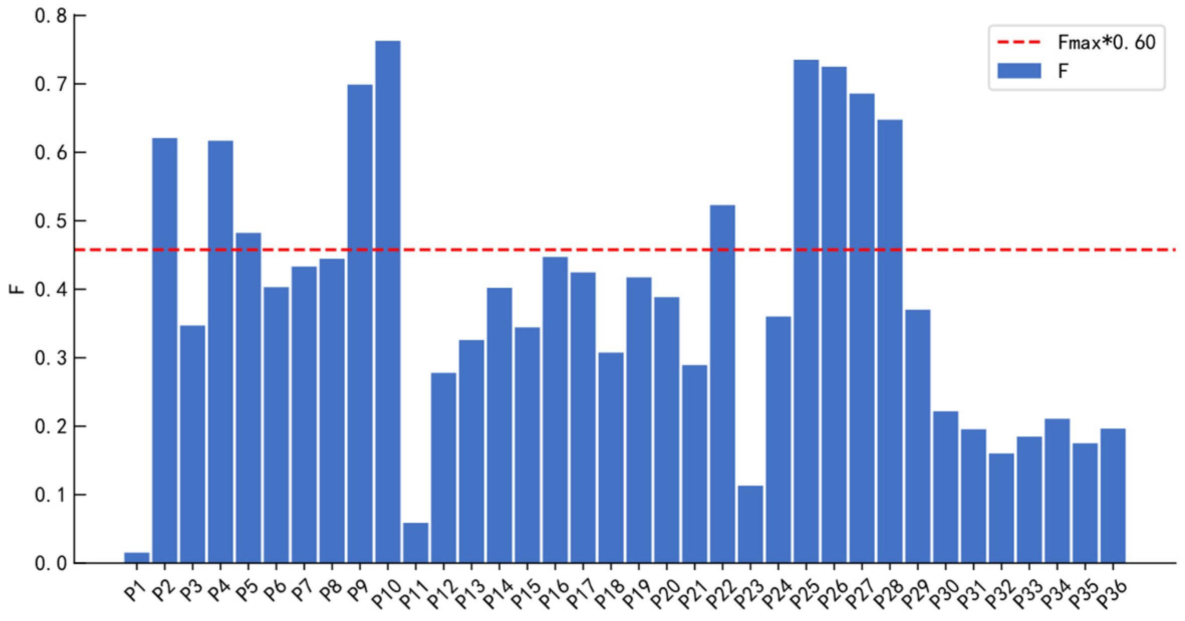
3.2. Comprehensive Index Screening

Not all extracted features are sensitive to the degradation process of rolling bearings. Therefore, feature selection is required. Since the degradation process of a bearing evolves over time and is irreversible, an effective degradation feature should exhibit strong temporal correlation and monotonicity. Monotonicity and correlation [10] are used to construct a comprehensive index (F) for feature selection, eliminating those features that are insensitive to the degradation process and creating a sensitive feature set. A higher F value indicates that the corresponding feature is more sensitive to bearing degradation. The calculations of monotonicity, correlation, and the composite index are as follows:

Monotonicity:

$$F_{mon}=\left|{\displaystyle \frac{Num of df>0}{T-1}}-{\displaystyle \frac{Num of df<0}{T-1}}\right|$$

(14)

where $df$ represents the differential between adjacent values in the feature curve, $T$ denotes the length of the feature data series, and $Num of$ denotes the count function, which calculates the number of elements satisfying a given condition.

Correlation:

$$F_{cor}={\displaystyle \frac{\left|{\sum }_{i=1}^n\left(x_i-\overline{x}\right)\left(y_i-\overline{y}\right)\right|}{\sqrt{{\sum }_{i=1}^n{\left(x_i-\overline{x}\right)}^2{\sum }_{i=1}^n{\left(y_i-\overline{y}\right)}^2}}}$$

(15)

where $x_i$ and $y_i$ represent the i-th elements of the feature vector and the RUL label, respectively, $\overline{x}$ and $\overline{y}$ represent the mean values of the feature vector and the RUL labels, respectively, and $n$ denotes the sequence length.

Aggregative indicator:

$$\begin{array}{c}F=w_1{F}_{mon}\left(x\right)+w_2{F}_{cor}\left(x\right)\end{array}$$

(16)

$$\begin{array}{c}{\sum }_{k=1}^2{w}_k=1,w_k>0\end{array}$$

(17)

where $x$ denotes the feature vector, and $w_k$ represents the weight corresponding to each evaluation metric. According to reference [10], $w_1$ is set to 0.3 and $w_2$ to 0.7. F denotes the comprehensive score of the feature.

3.3. Hierarchical Clustering Adaptively Removes Redundant Features

If the similarity between features is excessively high, the information they contain is largely redundant. This not only increases computational complexity but may also negatively affect the prediction performance of subsequent models. Therefore, it is essential to perform classification and reduction on the initially selected feature set. In this study, a redundancy elimination method based on the combination of hierarchical clustering and the elbow method is proposed. Given a feature set with a total of n features and a target number of clusters $K$, the procedure is illustrated in Figure 5, with the specific steps outlined as follows:

Step 1: Compute the distance matrix as defined in Section 2.1.

Step 2: Use the distance matrix as the input to the hierarchical clustering algorithm to perform agglomerative clustering. Obtain clustering results for different values of $K$ (where $K$ = 2, 3, 4, …, n) from the resulting dendrogram.

Step 3: Based on the clustering results from Step 2 and Formula (2), calculate the sum of squared errors for $K$ clusters and plot the elbow graph (where $K$ = 2, 3, 4, …, n).

Step 4: Determine the optimal number of clusters $K$ by identifying the “elbow point” on the curve using a combination of visual inspection and slope change analysis.

Step 5: Trim the dendrogram to obtain $K$ clusters according to the determined number of clusters.

Step 6: Select the optimal feature within each cluster as the cluster representative and construct the optimal feature set from these representatives.

3.4. Transformer–GRU Combination Model

To fully explore the relationship between the bearing degradation process and the RUL, a Transformer–GRU hybrid model is constructed, as illustrated in Figure 6. After inputting the data into the model, the multi-head attention mechanism in the Transformer encoder is first employed to capture various dependencies across different time steps in parallel subspaces [27]. This allows the original input feature sequences to be transformed into high-level feature representations rich in contextual information. Subsequently, the GRU, with its strong ability to capture temporal dependencies and trend patterns in sequential data [37], is used to extract the degradation trends from these high-level features. Finally, a fully connected layer maps the extracted features to the bearing’s RUL.

The mean absolute error (MAE) and root mean square error (RMSE) [6] are employed as evaluation metrics to assess the prediction performance of the proposed model. Their definitions are given in Equations (18) and (19), respectively:

$$\begin{array}{c}MAE={\displaystyle \frac{1}{m}}{\sum }_{i=1}^m\left|y_i-{\widehat{y}}_i\right|\end{array}$$

(18)

$$\begin{array}{c}RMSE=\sqrt{{\displaystyle \frac{{\sum }_{i=1}^m{\left(y_i-{\widehat{y}}_i\right)}^2}{m}}}\end{array}$$

(19)

where $m$ denotes the number of samples, $y_i$ represents the predicted value, and ${\widehat{y}}_i$ denotes the true value.

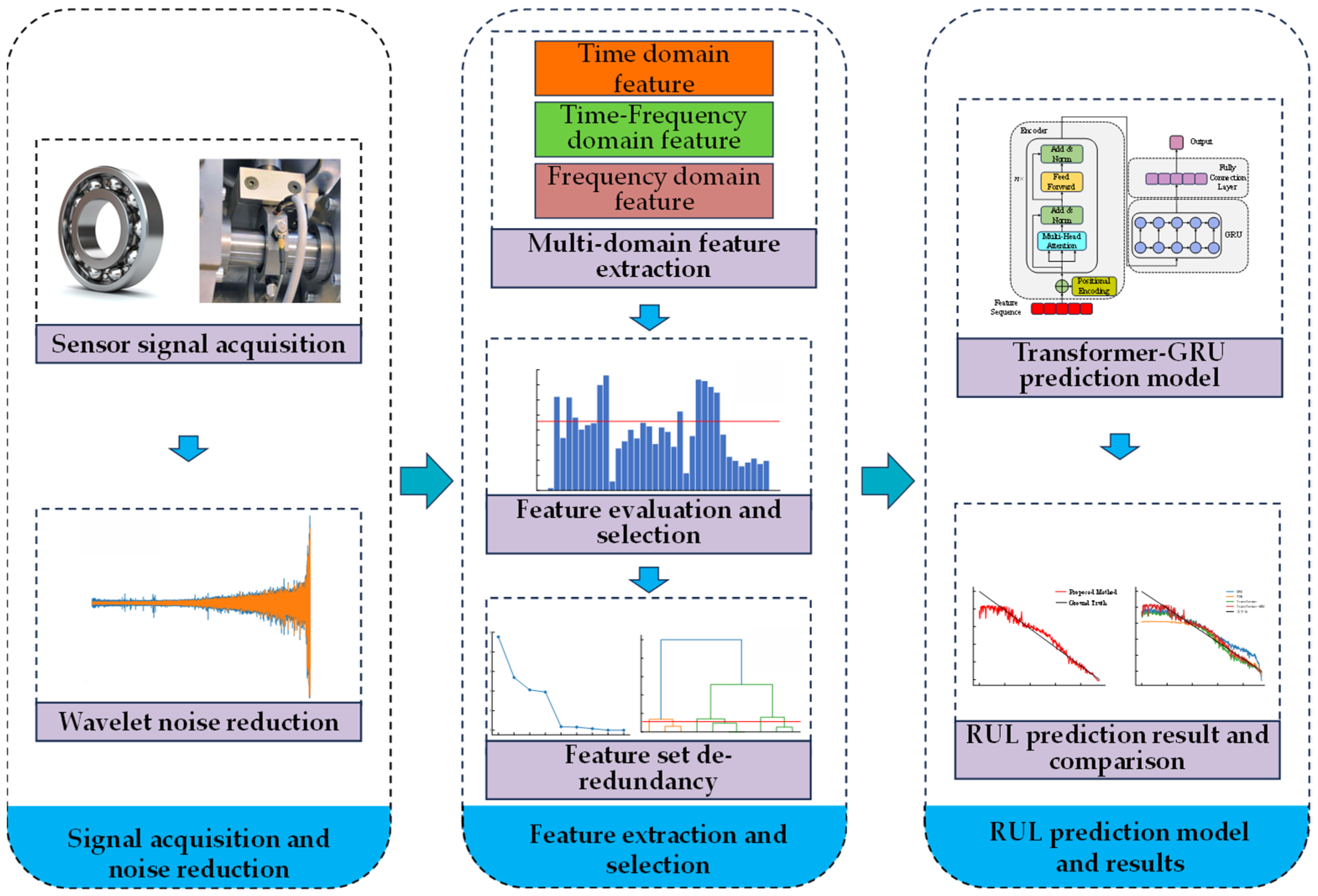
3.5. Process of the Proposed Method

The flowchart of the proposed method for rolling bearing RUL prediction is illustrated in Figure 7, and the specific steps are as follows:

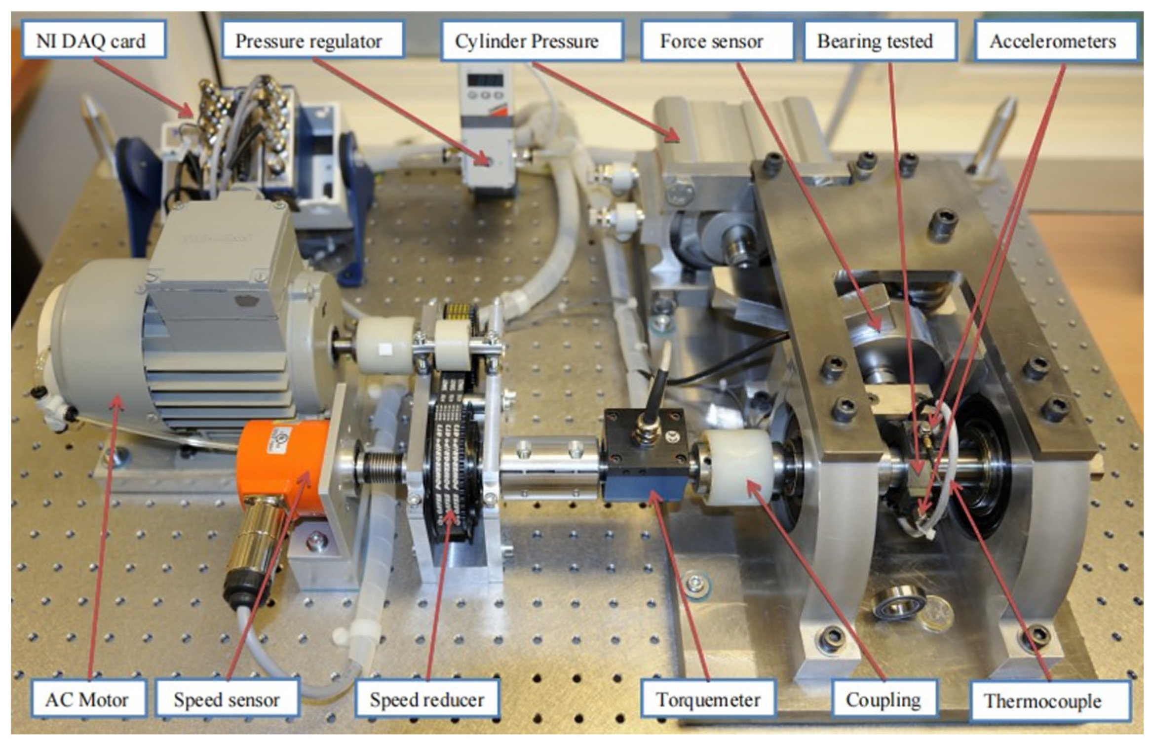
Step 1: Signal acquisition and denoising: Vibration signals of the full life cycle of the bearing are collected using an acceleration sensor. Wavelet denoising is applied to reduce noise in the original signals.

Step 2: Feature extraction: Time-domain, frequency-domain, and time–frequency-domain features are extracted from the denoised signals to form the original feature set, which is then smoothed and normalized.

Step 3: Feature selection: Based on a composite index constructed from monotonicity and correlation, features insensitive to bearing degradation are filtered out to form a sensitive feature set.

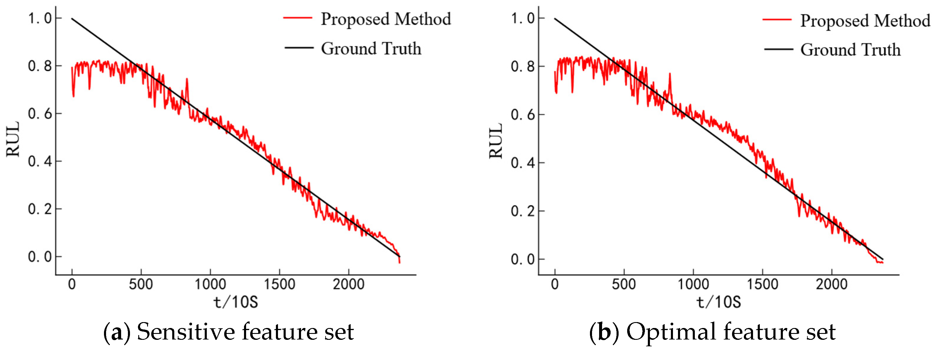
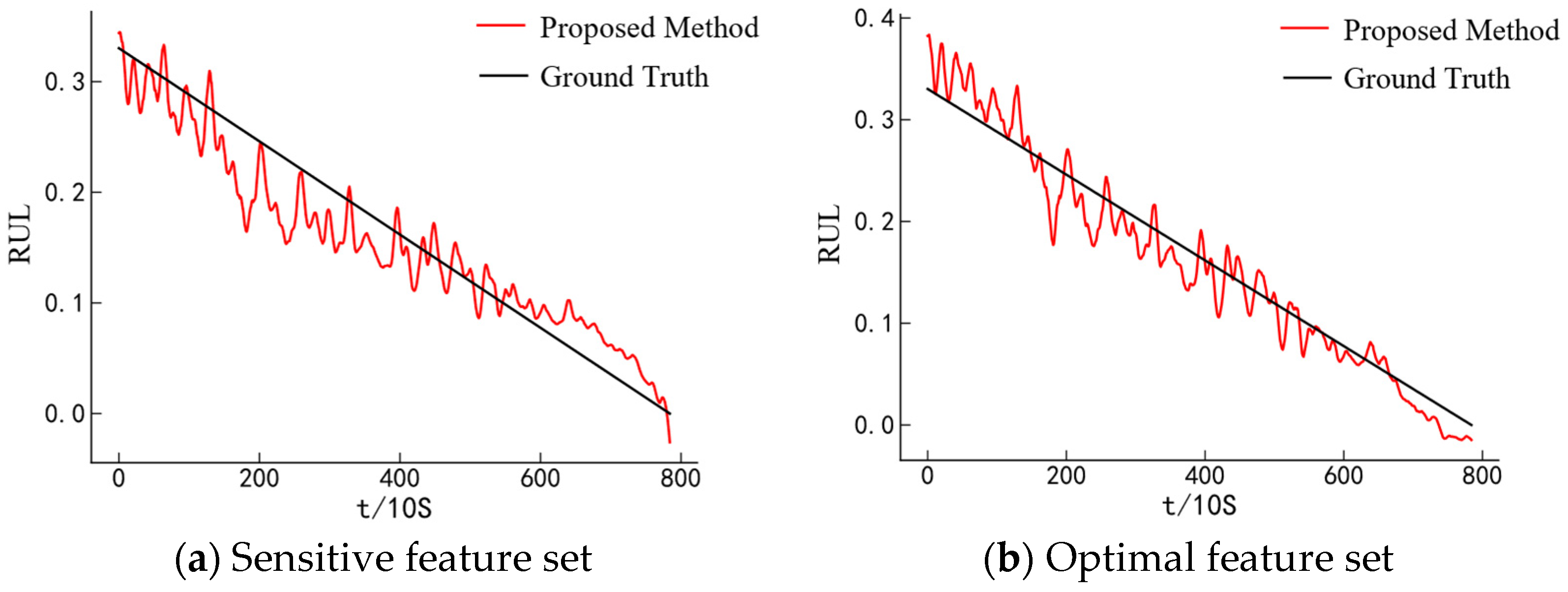
Step 4: Feature redundancy reduction: A hierarchical clustering method combined with the elbow method is employed to adaptively reduce redundancy in the sensitive feature set, resulting in the optimal feature set.

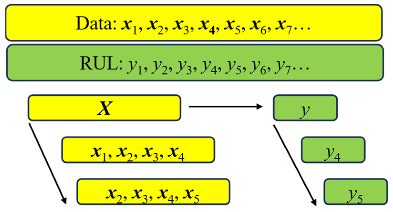
Step 5: Model training: The optimal feature set is used as input data for model training. The ratio of RUL to the total life cycle is used as the label.

Step 6: Model testing: The test set is fed into the trained model to predict the corresponding RUL labels, and the model performance is evaluated accordingly.

4. Implementation of RUL Prediction Based on Proposed Method

4.1. Dataset Description

To verify the effectiveness of the proposed method, the IEEE PHM 2012 public dataset [38] was employed for validation. This dataset was collected from the Pronostia experimental platform developed by the FEMTO-ST Institute, and the structure of the test rig is shown in Figure 8. The experimental platform is functionally divided into three main components: the rotation unit, the loading unit, and the measurement unit.

Rotation unit: This section primarily consists of an asynchronous motor, a gear reducer, couplings, and a drive shaft. The asynchronous motor has a rated power of 250 W and a rated speed of 2830 rpm. The motor’s rotational motion is transmitted to the supporting bearings through the gearbox, couplings, and shaft. The rotational speed and direction of the motor can be adjusted via a control interface to accommodate different experimental conditions with varying rotational speeds. Loading unit: This unit is composed of a pneumatic cylinder, pressure regulator, force sensor, and lever arm. The force generated by the pneumatic cylinder is amplified through the lever arm and applied to the outer ring of the bearing, imposing a high radial load to accelerate bearing degradation and failure. The pressure regulator allows for the adjustment of the applied force to meet different load condition requirements. Measurement unit: This section includes a set of sensors and a data acquisition card to monitor and record the operational state of the bearing, thereby capturing its degradation process. The acceleration sensor used is a DYTRAN3035B, with a measurement range of 50 g and a sensitivity of 100 mV/g. The temperature sensor is a platinum RTD100 (PROSENSOR), with detailed specifications available in reference [38].

The experiment recorded horizontal and vertical vibration signals throughout the degradation process of the bearings. When the amplitude of the measured vibration signal continuously exceeded 20 g, the bearing was considered to have reached complete failure, and the experiment was terminated. The sampling frequency was 25.6 kHz, the sampling duration was 0.1 s, and the sampling interval was 10 s. The experimental dataset includes three different operating conditions and a total of 17 rolling bearings. Detailed information is provided in

Table 2. Data of PHM2012.

Working Condition	Rotational Speed (rpm)	Radial Load (kN)	Bearing Data
1	1800	4	Bearing 1-1, Bearing 1-2, Bearing 1-3, Bearing 1-4, Bearing 1-5, Bearing 1-6, Bearing 1-7
2	1650	4.2	Bearing 2-1, Bearing 2-2, Bearing 2-3, Bearing 2-4, Bearing 2-5, Bearing 2-6, Bearing 2-7
3	1500	5	Bearing 3-1, Bearing 3-2, Bearing 3-3

. The first bearing under Condition 1 is denoted as B1-1, and the remaining bearings are labeled accordingly.

Three groups of experiments were conducted in this study, and the detailed division of the training and testing sets is shown in

Table 3. Experimental datasets.

Experimental Group	Training Set	Testing Set
1	B1-1	B1-3
2	B2-2	B2-1
3	B2-7	B2-6

. Each training or testing set contains the full life cycle data of the corresponding bearing. According to the findings of reference [39], horizontal vibration signals carry richer information; therefore, horizontal vibration signals were selected for subsequent analysis. A sliding window approach was adopted to convert the optimal feature sequences into sample data, as illustrated in Figure 9. In the figure, $x_1$ denotes the multidimensional feature vector at the first time point in the bearing life cycle, and $y_1$ represents the corresponding RUL label at that time. The sliding window length defines the number of data points included in a single sample, and the step size specifies the interval between two adjacent windows. To maximize data utilization, the step size was set to 1.

The proposed model takes the processed feature sample data as the input and outputs the normalized RUL of the bearing. A model output value of 0 indicates that the bearing has reached complete failure.

4.2. Feature Extraction and Selection

During acquisition, vibration signals are often affected by noise. To remove meaningless components, wavelet decomposition and reconstruction were applied. Taking Experiment Group 1 as an example, the signal of bearing B1-1 was denoised using a discrete wavelet transform. The Daubechies 5 wavelet was chosen as the mother wavelet, and the signal was decomposed into three levels. The reconstructed signal after denoising is shown in Figure 10. It is clearl that the denoised signal was smoother with fewer outliers.

Thirty-six features, as described in Section 3.1, were extracted from the denoised signal. To improve prediction accuracy and eliminate the influence of different feature magnitudes, the extracted features were smoothed using the Savitzky–Golay filter. Subsequently, the features were normalized to the range [0, 1]. The F-value for each feature was calculated according to Equation (16), and the results are shown in Figure 11. A threshold of 0.6 was set based on the highest-scoring features to filter out insensitive features. The selected features were {P2, P4, P5, P9, P10, P22, P25, P26, P27, P28}, which are presented in Figure 12.

Upon examining the results, it was observed that all features were sensitive to changes occurring throughout the entire life cycle of the bearing. For instance, the time-domain energy feature P4 remained relatively stable and low in magnitude during the early phase of bearing operation, corresponding to the normal running stage. This observation is consistent with the literature [32], reporting that vibration signals are steady and exhibit low amplitudes during this period. After approximately 15,000 s, the magnitude of P4 began to increase, albeit with a gentle slope, suggesting a gradual rise in signal energy. This aligns with the literature [32], reporting that amplitude fluctuations emerge as degradation begins. Around 27,000 s, a sharp increase in energy was observed, which corresponded to the abrupt changes in vibration amplitude typically seen during the terminal failure phase. These results confirm that the selected features effectively captured the bearing’s degradation behavior over its full service life.

However, the rate at which trends change differed across the features, likely due to the varying types of degradation information encoded in each feature. Additionally, some features, such as P2 and P4, exhibited very similar trends. Figure 13 displays the Pearson correlation matrix heatmap, which illustrates the relationships between features. From Figure 13, it is evident that some features were highly similar, with P2 and P4 being linearly correlated.

Although the comprehensive index effectively filtered out features that were insensitive to bearing degradation, it did not account for the relationships among features. Excessive correlation between features leads to redundant information within the feature set, which not only increases its dimensionality but also adds to the model’s complexity and computational burden [40]. To address this issue, further feature selection was performed. Based on hierarchical clustering combined with the elbow method proposed in Section 3.3, clustering analysis was conducted on the sensitive feature set. The resulting elbow plot is shown in Figure 14a. As observed, the inflection point occurred at $K$ = 6. Although the error reduction rate was faster at $K$ = 3, the decline in error did not level off after this point, which does not conform to the typical “elbow” pattern. Therefore, the dendrogram was pruned into six clusters, as shown in Figure 14b. The final clustering results are presented in

Table 4. Feature clustering results.

Cluster Number	1	2	3	4	5	6
Feature	P2, P4, P22	P5	P9	P10, P26	P25, P27	P28

. The feature with the highest F-score in each cluster was selected as the representative, forming the following optimal feature set: {P2, P5, P9, P10, P25, P28}.

4.3. Experimental Environment and Hyperparameter Selection

The experiments were conducted using the PyTorch 2.3.0 framework to build the deep learning model. The implementation language was Python 3.9, and PyCharm 2025.1.1 was used as the development environment. The software environment was configured with CUDA 12.6. The hardware setup included a Windows 11 operating system, an Intel i5-12500H CPU, and 16 GB of RAM. The selection of hyperparameters and structural parameters plays a critical role in model performance. Additionally, the impact of the input sequence length on prediction accuracy was taken into consideration. The Adam optimizer was employed, and extensive experiments were conducted to optimize the parameter combinations. The optimal configuration was determined based on the RMSE between the predicted and actual values. The final parameter settings are summarized in

Table 5. Parameter setting.

Parameter	Value
Batch size	16
Learning rate	0.01
Epoch	300
Number of multiple attention heads	2
The number of hidden units of GRU	128, 64
Window length	8

.

To enable a more detailed comparison of the prediction performance across different feature sets and models, the bearing RUL was divided into three stages, referred to as the early stage, middle stage, and late stage.

4.4. Experimental Verification and Analysis

4.4.1. Experimental Result Analysis

The prediction results of all tested bearings in the experiment are shown in Figure 15. It can be observed that the predicted values fluctuated around the actual values, and the overall trends were closely aligned, which validates the effectiveness of the proposed method. Further analysis revealed that in all three experimental groups, the predicted RUL remained nearly flat during the initial stage, indicating that the model struggled to capture the degradation trend at this phase. As noted in previous research on early-stage RUL prediction of rolling bearings [41], the degree of degradation is minimal in the early operational phase, leading to negligible variations in the acquired signals. Consequently, the extracted features show little change, making it difficult for the prediction model to learn meaningful degradation patterns, and resulting in flat RUL predictions. A comparative analysis revealed that the prediction results for bearing B1-3 exhibited relatively small fluctuations, whereas bearings B2-1 and B2-6 showed greater volatility. This may be attributed to the fact that B1-3 underwent a gradual degradation process, while B2-1 and B2-6 exhibited abrupt degradation behaviors. At the same time, this is consistent with the difficulties in predicting the remaining useful life of bearings with sudden failure patterns, as highlighted in the literature [28].

4.4.2. Comparison Before and After Feature Clustering Reduction

To validate the necessity and effectiveness of feature set reduction using hierarchical clustering, a comparison was conducted by inputting both the sensitive feature set and the optimal feature set into the model while keeping other experimental parameters and conditions constant. Taking Experiment Group 1 as an example, the prediction results are presented in Figure 16 and

Table 6. The whole life evaluation index of the same feature set.

Evaluating Indicator	Sensitive Feature Set	Optimal Feature Set
MAE	0.0433	0.0453
RMSE	0.0638	0.0632
Number of model parameters	294,400	225,908
Training time (s)	455.681	415.743

. As shown in Figure 16, in the early stages of prediction, neither feature set performed well in predicting the RUL. In the middle stages, the sensitive feature set demonstrated better prediction performance. In the later stages, the optimal feature set not only provided more accurate predictions but also eliminated any prediction delay. According to the results in Table 6, although the MAE and RMSE values of the optimal feature set were similar to those of the sensitive feature set, this indicates that the optimal feature set contained a comparable amount of information to the sensitive feature set. The proposed method effectively removed redundant features from the feature set without losing useful information. Compared to the sensitive feature set, the optimal feature set resulted in an 8.61% reduction in model training time and a 23.26% reduction in model parameters. This demonstrates that by refining the sensitive feature set, the model’s training efficiency was improved, and its complexity was reduced. The experimental results confirm that the proposed feature redundancy removal method is both necessary and effective for feature set construction.

To verify the superiority of the proposed method, a comparative experiment was conducted between the proposed approach and the Max-Relevance Min-Redundancy method [42]. The experimental results are shown in the

Table 7. Comparative analysis of various feature selection methods.

Evaluating Indicator	Max-Relevance Min-Redundancy Method	Proposed Method
MAE	0.0504	0.0453
RMSE	0.0682	0.0632
Number of model parameters	260,054	225,908
Training time (s)	430.674	415.743

. It can be observed that the proposed method achieved smaller prediction errors, with a 13.13% reduction in model parameters and a 3.5% decrease in training time. This is because the Max-Relevance Min-Redundancy method emphasizes high correlation between the selected features and the target variable, but it still retains some redundant features. In contrast, the proposed method ensured a relatively high correlation with the target variable during the initial screening stage. Then, by employing hierarchical clustering to further eliminate redundancy within the feature set, a more optimal and compact feature subset was obtained.

Considering that the later stages of rolling bearing life are critical for bearing failure, a further analysis of the prediction performance of the two feature sets in the RUL prediction during the later stages was conducted. The prediction results for the two feature sets are shown in Figure 17 and

Table 8. The later evaluation index of life prediction of different feature sets.

Evaluating Indicator	Sensitive Feature Set	Optimal Feature Set
MAE	0.0259	0.0187
RMSE	0.0312	0.0232

. As depicted in Figure 17, the predictions using the optimal feature set were more aligned with the true RUL of the bearing, and no lagging phenomenon was observed. According to Table 8, compared with the sensitive feature set, the MAE of the optimal feature set was reduced by 27.8%, and the RMSE was reduced by 25.6%. Therefore, feature redundancy removal from the sensitive feature set can effectively improve the prediction accuracy of the bearing RUL in the later stages. This further confirms the effectiveness and necessity of the proposed method.

4.4.3. Comparison of Different Models

To verify the superiority of the proposed combined model, single models such as GRU, Transformer, and TCN were selected as comparison models, and a comparative experiment was conducted using MAE and RMSE as evaluation metrics. Additionally, the results were compared with those from similar studies [6,43]. The prediction results for Experiment Group 1 are shown in Figure 18, and the results for all experimental groups are presented in

Table 9. Evaluation indexes of different models.

Model	Evaluating Indicator	B1-3	B2-1	B2-6	Average
GRU	MAE	0.0750	0.1094	0.1495	0.1113
	RMSE	0.0970	0.1321	0.1940	0.1410
TCN	MAE	0.0878	0.1195	0.1483	0.1185
	RMSE	0.1369	0.1549	0.1919	0.1612
Transformer	MAE	0.0646	0.0947	0.1391	0.0995
	RMSE	0.0924	0.1279	0.1831	0.1344
Reference [6]	MAE	0.0670	0.1950	0.0375	0.0998
	RMSE	0.0830	0.2610	0.0507	0.1316
Reference [43]	MAE	0.0560	0.1570	0.0720	0.0950
	RMSE	0.0700	0.1900	0.0940	0.1180
Proposed Method	MAE	0.0453	0.0885	0.1172	0.0836
	RMSE	0.0632	0.1209	0.1570	0.1137

. As shown in Figure 18, during the early stage of prediction, all models failed to predict accurately, but the Transformer–GRU model provided results closer to the true values. In the middle stage, all four models exhibited some lag. In the later stages, GRU still showed a lagging issue, while TCN performed better, although some lag occurred in the final stage. The Transformer model underestimated the actual values, which could lead to unnecessary actions in predictive maintenance. In contrast, the Transformer–GRU model’s predictions aligned closely with the true RUL.

According to Table 9, the proposed combined model reduced the average MAE by 24.9% and the average RMSE by 19.36% compared to GRU; reduced the average MAE by 29.4% and the average RMSE by 29.5% compared to TCN; and reduced the average MAE by 16.0% and the average RMSE by 15.4% compared to Transformer. These comparative results demonstrate that the proposed model achieved higher prediction accuracy. It can be concluded that the combined model proposed in this study achieved the highest prediction accuracy. Single models can only extract useful information from features from a single dimension, while the combined model proposed in this study allows the encoder part to extract local variation information from the degradation features by capturing the dependencies across time steps. GRU, on the other hand, can capture the macro trend information that evolves over time in different feature samples. This enables more efficient mining of the bearing degradation patterns and consequently improves the model’s prediction performance.

Compared with the improved models [43] and combined models [6] in the literature, the model proposed in this study achieved the best prediction performance with the lowest average error. In contrast to the approach in reference [6], which uses TCN, LSTM, and Transformer models to extract features from input data and then simply concatenates the features extracted by the different models, the combined model proposed in this study concatenates two models in series. By deepening the network, GRU further extracts features from the encoder’s output, thereby obtaining more advanced features and endowing the model with stronger expressive power. Reference [43] improves TCN by introducing attention mechanisms and multi-scale mechanisms. In comparison, the multi-head attention mechanism in the encoder of our model not only mines the dependencies across different time steps but also assigns greater weight to key time steps. The Transformer and GRU extract information from different dimensions, which, compared to multi-scale information, carries more comprehensive and rich information. Additionally, based on the experimental results of this study and those in the literature [43,44,45], it can be observed that the prediction error for Bearing 1-3 was the smallest, further confirming that the prediction of gradual-change bearings is less challenging than that of sudden-change bearings.

4.4.4. Generalization Verification

To verify the generalizability of the proposed method, the XJTU-SY full-life rolling bearing dataset was used for method validation. This dataset includes full-life cycle data for 15 bearings under three different operating conditions. The sampling frequency is 25.6 kHz, the sampling duration is 1.28 s, and the sampling interval is 1 min. The specific experimental procedure and details can be found in reference [46]. Bearings B2-2 and B2-3 were selected for training and testing using the same experimental setup and process as the PHM 2012 dataset. Bearing B2-2 was used as the training set, while B2-3 was used as the test set. The prediction results are shown in Figure 19 and

Table 10. Evaluation indexes of different models.

Model	MAE	RMSE
GRU	0.0885	0.1099
TCN	0.0797	0.1025
Transformer	0.0859	0.1123
Proposed Method	0.0674	0.0914

.

As shown in Figure 19, during the early prediction phase, all models failed to make accurate predictions. In the middle phase, all four models exhibited a certain degree of lag in their predictions, but GRU and the proposed model showed a lower level of lag. In the later prediction phase, both the TCN and Transformer models experienced lag, while GRU’s predicted values were too low, leading to potential waste in predictive maintenance. In contrast, the proposed model’s predictions were closest to the true values and did not exhibit any lag, making it more practical. From Table 10, it can be seen that the proposed model outperformed GRU with a 23.8% reduction in MAE and a 16.8% reduction in RMSE. Compared to TCN, MAE was reduced by 15.0% and RMSE by 10.8%. When compared to Transformer, MAE was reduced by 21.5% and RMSE by 18.6%. Through comparative analysis, it is further demonstrated that the proposed model offers higher prediction accuracy.

5. Conclusions

To address the issues of insufficient feature selection, feature redundancy, and low prediction accuracy of single models in traditional bearing RUL prediction methods, a novel approach is proposed that combines hierarchical clustering for feature selection and a Transformer–GRU hybrid model for RUL prediction. The method was validated using the PHM 2012 dataset, and the experimental results provide the following insights:

(1)

The proposed adaptive feature reduction method, which integrates hierarchical clustering with the elbow method, effectively eliminates redundant information in the feature set while avoiding the subjectivity associated with manually determining the number of clusters. Compared to the unreduced feature set, the reduced set exhibits lower inter-feature similarity and fewer dimensions, thereby reducing model complexity, enhancing training efficiency, and improving prediction accuracy in the later stages of bearing RUL prediction. These findings demonstrate the necessity of redundant feature removal. Furthermore, comparative experiments with other feature selection methods validate the superiority of the proposed approach.

(2)

The Transformer encoder and GRU-based hybrid model demonstrate stronger time-series modeling capabilities and better capture temporal dependencies compared to single models. This hybrid model can deeply explore the relationship between the extracted features and the RUL of bearings, leading to more accurate predictions of bearing RUL. Comparative analyses with models from related studies further highlight the effectiveness and superiority of the proposed model.

(3)

Bearings exhibiting abrupt degradation patterns pose greater challenges in RUL prediction due to the limited availability of degradation data, making them more difficult to predict than gradually degrading bearings. Additionally, early-stage RUL prediction is inherently more difficult, as signal features tend to show minimal variation during this period, hindering the model’s predictive accuracy.

(4)

The research in this paper, as well as the referenced studies, were conducted only on ball bearings, and thus, the findings are applicable solely to this type of rolling bearing. The applicability of the proposed methods to other types of rolling bearings requires further investigation and validation.

References

1. Lazovic, T.; Marinkovic, A.; Atanasovska, I.; Sedak, M.; Stojanovic, B. From Innovation to Standardization—A Century of Rolling Bearing Life Formula. Machines 2024, 12, 444. [Google Scholar] [CrossRef]
2. Pastukhov, A.; Timashov, E. Procedure for Simulation of Stable Thermal Conductivity of Bearing Assemblies. Adv. Eng. Lett. 2023, 2, 58–63. [Google Scholar] [CrossRef]
3. Li, J.; Luo, W.; Chen, W. Overview of Algorithms for Rolling Bearing Fault Diagnosis Based on Vibration Signal. J. Xi’an Technol. Univ. 2022, 42, 105–122. [Google Scholar] [CrossRef]
4. Lu, Z.; Dong, S.; Zhu, S.; Zou, S.; Huang, X. Fault Diagnosis of Cross-Working Rolling Bearing Based on Multi-source Depth Domain Self-adaptation. Mach. Tool Hydraul. 2024, 52, 230–238. [Google Scholar] [CrossRef]
5. Zhang, S. Summary of Prediction of Remaining Useful Life of Rolling Bearings. Intern. Combust. Engine Parts 2024, 18, 24–26. [Google Scholar] [CrossRef]
6. Zhang, G.; Jiang, D. Research on the Remaining Life Prediction Method of Rolling Bearings Based on Multi-Feature Fusion. Appl. Sci. 2024, 14, 1294. [Google Scholar] [CrossRef]
7. Paris, P.; Erdogan, F. A Critical Analysis of Crack Propagation Laws. J. Basic Eng. 1963, 85, 528–533. [Google Scholar] [CrossRef]
8. Forman, R.G. Study of Fatigue Crack Initiation from Flaws Using Fracture Mechanics Theory. Eng. Fract. Mech. 1972, 4, 333–345. [Google Scholar] [CrossRef]
9. Li, C.; Song, Y. A Study of the Applicability of Palmgren-Miner Criterion on the Fatigue Damage Accumulation of Concrete Offshore Platform. China Offshore Platf. 2001, 16, 1–4. [Google Scholar] [CrossRef]
10. Cao, X.; Zhang, F.; Zhao, J.; Duan, Y.; Guo, X. Remaining Useful Life Prediction of Rolling Bearing Based on Multi-Domain Mixed Features and Temporal Convolutional Networks. Appl. Sci. 2024, 14, 2354. [Google Scholar] [CrossRef]
11. Li, H.; Zou, Y.; Zeng, D.; Liu, Y.; Zhao, S.; Song, X. A New Method of Bearing Life Prediction Based on Feature Clustering and Evaluation. J. Vib. Shock 2022, 41, 141–150. [Google Scholar] [CrossRef]
12. Wu, Y.; Wei, K.; Yang, S. Residual Life Prediction of Rolling Bearings Based on GOA Optimization LSTM Network. Manufacturing Technol. Mach. Tool 2024, 5, 35–41. [Google Scholar] [CrossRef]
13. Wang, F.; Liu, X.; Deng, G.; Li, H.; Yu, X. Remaining Useful Life Prediction Method for Rolling Bearing Based on the Long Short-Term Memory Network. J. Vib. Meas. Diagn. 2020, 40, 303–309. [Google Scholar] [CrossRef]
14. Zhang, B.; Zhang, L.; Xu, J. Degradation Feature Selection for Remaining Useful Life Prediction of Rolling Element Bearings. Qual. Reliab. Eng. Int. 2016, 32, 547–554. [Google Scholar] [CrossRef]
15. Zhu, R.; Zhang, X.; Huang, Q.; Li, S.; Fu, Q. Predicting the Remaining Life of Centrifugal Pump Bearings Using the KPCA–LSTM Algorithm. Energies 2024, 17, 4167. [Google Scholar] [CrossRef]
16. Li, X.; Yang, Z.; Ren, J. Improved Naive Bayes Algorithm Based on Dual Feature Selection of Mutual Information and Hierarchical Clustering. Meas. Control Technol. 2022, 41, 36–40. [Google Scholar] [CrossRef]
17. Feng, Z.; Wang, Z.; Liu, X.; Li, J. Rolling Bearing Performance Degradation Assessment with Adaptive Sensitive Feature Selection and Multi-Strategy Optimized SVDD. Sensors 2023, 23, 1110. [Google Scholar] [CrossRef]
18. Yang, B.; Liu, R.; Zio, E. Remaining Useful Life Prediction Based on a Double-Convolutional Neural Network Architecture. IEEE Trans. Ind. Electron. 2019, 66, 9521–9530. [Google Scholar] [CrossRef]
19. Song, L.; Wu, J.; Wang, L.; Chen, G.; Shi, Y.; Liu, Z. Remaining Useful Life Prediction of Rolling Bearings Based on Multi-Scale Attention Residual Network. Entropy 2023, 25, 798. [Google Scholar] [CrossRef]
20. Cao, S.; Xu, Y.; Xie, T.; Wang, L. Prediction of Bearing Residual Life Based on Multi Information Fusion and GRU. Mach. Tool Hydraul. 2023, 51, 164–168. [Google Scholar] [CrossRef]
21. Qiu, H.; Niu, Y.; Shang, J.; Gao, L.; Xu, D. A Piecewise Method for Bearing Remaining Useful Life Estimation Using Temporal Convolutional Networks. J. Manuf. Syst. 2023, 68, 227–241. [Google Scholar] [CrossRef]
22. Zhou, Z.; Liu, L.; Song, X.; Chen, K. Remaining Useful Life Prediction Method of Rolling Bearing Based on Transformer Model. J. Beijing Univ. Aeronaut. Astronaut. 2023, 49, 430–443. [Google Scholar] [CrossRef]
23. Ye, Y.; Li, D.; Wang, S.; Zheng, T.; Su, Y. Pilot Protection for New Energy Access to Power Grid Based on Generalized S Transform and Pearson Correlation Coefficient. J. Electr. Power Sci. Technol. 2024, 39, 194–202. [Google Scholar] [CrossRef]
24. He, X.; He, F.; Fan, Y.; Chen, H. Visualized Determination Mode for Clustering Quantity of High-Dimensional Data. J. Shenyang Aerosp. Univ. 2024, 41, 71–84. [Google Scholar] [CrossRef]
25. Pan, P.; Liu, H.; Wang, R. LSTM Wind Power Prediction Based on Combined Data Cleansing Algorithm of Self-Adaptive DBSCAN and K-Means Clustering. Proc. CSU-EPSA 2024, 36, 59–66. [Google Scholar] [CrossRef]
26. Vaswani, A.; Shazeer, N.; Parmar, N.; Uszkoreit, J.; Jones, L.; Gomez, A.N.; Kaiser, L.; Polosukhin, I. Attention Is All You Need. arXiv 2023, arXiv:1706.03762v7. [Google Scholar]
27. Li, D.; Liu, X.; Liu, J.; Chen, S. Intrusion Detection Research Combining Transformer and Bi-directional GRU [OL]. Comput. Eng. Appl. 2024, 1–11. Available online: https://link.cnki.net/urlid/11.2127.TP.20240819.1043.010 (accessed on 8 May 2025).
28. Zeng, L. Study on Multi-stage Prediction Method of Remaining Useful Life of Rolling Bearing Based on Transformer Health Indicator. Master’s Thesis, Chongqing University, Chongqing, China, 2022. [Google Scholar] [CrossRef]
29. Chung, J.; Gulcehre, C.; Cho, K.; Bengio, Y. Empirical Evaluation of Gated Recurrent Neural Networks on Sequence Modeling. arXiv 2014, arXiv:1412.3555. [Google Scholar]
30. Lei, W.; Yan, H.; Li, Q.; Li, Y.; Zheng, P. Unsupervised Tool Anomaly Detection Based on AGRU Autoencoder. Mach. Tool Hydraul. 2024, 52, 30–37. [Google Scholar] [CrossRef]
31. Chen, C.; Guo, J.; Qu, H.; Wang, F.; Wang, P. Fault Diagnosis of Rolling Bearing Based on Multi-scale Convolutional Neural Network and GRU [OL]. Bearing 2023, 1–11. Available online: https://link.cnki.net/urlid/41.1148.TH.20231012.1102.002 (accessed on 8 May 2025).
32. Yang, Y. Study on Predicting the Remaining Service Life of Rolling Bearing Based on Signal Processing Method by Vibration Signal. Master’s Thesis, Beijing University of Chemical Technology, Beijing, China, 2016. [Google Scholar]
33. Yan, C. Degradation Assessment and Residual Life Prediction of Rolling Bearings Based on Multiple Features. Master’s Thesis, School of Mechatronics Engineering, Chengdu, China, 2016. [Google Scholar]
34. Yin, G. Research on Useful Life Prediction of Rolling Bearing Based on Pearson-KPCA Multi-Feature Fusion. Master’s Thesis, Harbin University of Science and Technology, Harbin, China, 2021. [Google Scholar] [CrossRef]
35. Wan, G.; Pei, J.; Qi, M. Experimental Studies on Relationship Between Rolling Bearing Life and State Characteristic Parameter. Coal Mine Mach. 2010, 31, 68–70. [Google Scholar] [CrossRef]
36. Lei, Y.; He, Z.; Zi, Y.; Hu, Q. Fault Diagnosis of Rotating Machinery Based on Multiple ANFIS Combination with GAs. Mech. Syst. Signal Proc. 2007, 21, 2280–2294. [Google Scholar] [CrossRef]
37. Zheng, X.; Qian, Y.; Wang, S. GRU Prediction for Performance Degradation of Rolling Bearings Based on Optimal Wavelet Packet and Mahalanobis Distance. J. Vib. Shock 2020, 39, 39–46, 63. [Google Scholar] [CrossRef]
38. Nectoux, P.; Gouriveau, R.; Medjaher, K.; Ramasso, E.; Morello, B.; Zerhouni, N.; Varnier, C. PRONOSTIA: An Experimental Platform for Bearings Accelerated Degradation Tests. In Proceedings of the PHM 2012: IEEE Conference on Prognostics and Health Management, Denver, CO, USA, 18–21 June 2012; pp. 1–8. [Google Scholar]
39. Singleton, R.K.; Strangas, E.G.; Aviyente, S. Extended Kalman Filtering for Remaining-Useful-Life Estimation of Bearings. IEEE Trans. Ind. Electron. 2014, 62, 1781–1790. [Google Scholar] [CrossRef]
40. Wang, T.; Hu, Z.; Zhan, H. A Novel Unsupervised Feature Selection Method. J. Shandong Univ. (Nat. Sci.) 2024, 59, 130–140. [Google Scholar]
41. Hao, J.; Wang, Y.; Guo, Q.; Zhang, W. Remaining Useful Life Prediction Algorithm for Rolling Bearing in the Early Stage. Comput. Eng. 2024, 50, 48–58. [Google Scholar] [CrossRef]
42. Leng, T.; Ye, R.; Xu, S. The Two-Staged Text Feature Selection Method with Maximum Correlation and Minimum Redundancy. J. Anhui Univ. Sci. Technol (Nat. Sci.) 2024, 44, 83–89. [Google Scholar] [CrossRef]
43. Wang, S.; Liu, Y.; Liu, J.; Sun, H.; Wen, W. Research on Bearing Life Prediction Algorithm Based on Improved Multi-Scale Temporal Convolutional Network. Control Eng. China 2024. [Google Scholar] [CrossRef]
44. Wang, Y.; Deng, L.; Zheng, L.; Gao, R. Temporal convolutional network with soft thresholding and attention mechanism for machinery prognostics. J. Manuf. Syst. 2021, 60, 512–526. [Google Scholar] [CrossRef]
45. Cao, Y.; Ding, Y.; Jia, M.; Tian, R. A novel temporal convolutional network with residual self-attention mechanism for remaining useful life prediction of rolling bearings. Reliab. Eng. Syst. Saf. 2021, 215, 107813. [Google Scholar] [CrossRef]
46. Wang, B.; Lei, Y.; Li, N.; Li, N. A Hybrid Prognostics Approach for Estimating Remaining Useful Life of Rolling Element Bearings. IEEE Trans. Reliab. 2018, 69, 401–412. [Google Scholar] [CrossRef]
Figure 1. Agglomerative method diagram, different letters in the figure denote different features, while the arrows indicate the directions of clustering.
Applsci 15 05369 g001
Figure 2. Encoder structure.
Applsci 15 05369 g002
Figure 3. Multi-head attention structure.
Applsci 15 05369 g003
Figure 4. Structure diagram of GRU.
Applsci 15 05369 g004
Figure 5. Hierarchical clustering to redundancy flow chart.
Applsci 15 05369 g005
Figure 6. Structure diagram of Transformer–GRU combined model.
Applsci 15 05369 g006
Figure 7. Graphical abstract.
Applsci 15 05369 g007
Figure 8. Pronostia experimental platform.
Applsci 15 05369 g008
Figure 9. Sliding window diagram.
Applsci 15 05369 g009
Figure 10. Comparison diagram before and after signal noise reduction.
Applsci 15 05369 g010
Figure 11. Comprehensive index screening results.
Applsci 15 05369 g011
Figure 12. Sensitive feature set.
Applsci 15 05369 g012
Figure 13. Sensitive feature set correlation coefficient heat map.
Applsci 15 05369 g013
Figure 14. (a) Clustering error elbow diagram; (b) sensitive feature clustering tree diagram.
Applsci 15 05369 g014
Figure 15. Different bearing RUL prediction results.
Applsci 15 05369 g015
Figure 16. Comparison diagram of whole life prediction of different feature sets.
Applsci 15 05369 g016
Figure 17. Late comparison diagram of life prediction of different feature sets.
Applsci 15 05369 g017
Figure 18. Comparison of different model prediction results.
Applsci 15 05369 g018
Figure 19. Comparison of different model predictions.
Applsci 15 05369 g019