Metric Scaling and Extrinsic Calibration of Monocular Neural Network-Derived 3D Point Clouds in Railway Applications

Featured Application

Monocular depth estimation models often produce non-metric (relative) depth, and even when they aim to predict metric depth, they tend to perform poorly on unseen data, as demonstrated in our study. However, many real-world applications of monocular depth estimation require accurate metric measurements, for example, to verify compliance with legal regulations. As part of the EU-funded research project BerDiBa, we investigated the calibration of depth estimation models for metric accuracy in the railway domain. Our goal was to establish a foundation for a specific use case: measuring the encroachment of vegetation into the structural gauge. This is a critical challenge, as such vegetation can obstruct and distort sensor data or, in the case of hard wooden plants, even cause physical damage to trains. We aimed to develop a method that enables reliable metric scaling of any recent monocular depth estimation model, regardless of its training data or camera parameters, in order to meet legal requirements.

Abstract

Three-dimensional reconstruction using monocular camera images is a well-established research topic. While multi-image approaches like Structure from Motion produce sparse point clouds, single-image depth estimation via machine learning promises denser results. However, many models estimate relative depth, and even those providing metric depth often struggle with unseen data due to unfamiliar camera parameters or domain-specific challenges. Accurate metric 3D reconstruction is critical for railway applications, such as ensuring structural gauge clearance from vegetation to meet legal requirements. We propose a novel method to scale 3D point clouds using the track gauge, which typically only varies in very limited values between large areas or countries worldwide (e.g., $1.435$ m in Europe). Our approach leverages state-of-the-art image segmentation to detect rails and measure the track gauge from a train driver’s perspective. Additionally, we extend our method to estimate a reasonable railway-specific extrinsic camera calibration. Evaluations show that our method reduces the average Chamfer distance to LiDAR point clouds from $1.94$ m (benchmark UniDepth) to $0.41$ m for image-wise calibration and $0.71$ m for average calibration.

1. Introduction

Aligned with advancements in the automotive industry, the railway sector is increasingly focusing on autonomous driving and predictive maintenance. A key technique is 3D reconstruction of the structural gauge, enabling tasks such as detecting vegetation encroaching on the driving corridor. Large, wooden vegetation can damage trains, while smaller, softer vegetation may obscure sensors and distort data. This challenge was addressed in the recent EU-founded research project BerDiBa (Berliner Digitaler Bahnbetrieb engl. Berlin Digital Rail Operation) [1].

For such tasks, the camera sensor is particularly valuable due to its cost efficiency and ability to provide dense data. However, this advantage comes at the cost of dimensional reduction, as images are inherently 2D. Traditional methods to address this issue, like Structure from Motion (SfM), require multiple consecutive images and often yield sparse 3D point clouds. Advancements in machine learning have tackled this limitation by enabling pixelwise depth estimation from single images, yielding a denser and more detailed 3D point cloud. However, many of these models predict relative depth to remain independent of specific camera parameters, which limits their usability for tasks like inspecting the structural gauge that is normally defined by metric requirements. For instance, in Germany, legal regulations mandate a vegetation-free zone of 1 m (Wachstumszuschlag) beyond the structural gauge to reduce risks from vegetation growth.

Our evaluation of the latest metric depth estimation model [2] revealed an average Chamfer distance of $1.94$ m compared to LiDAR across all 45 scenes in the railway dataset OSDaR23 [3]. This level of accuracy fails to meet the legal requirements for detecting structural gauge clearance from vegetation. To improve accuracy, we leverage the fact that at least one track is typically visible when recording the structural gauge from the driver’s perspective. The metric gauge of this track is generally well-known, as it varies only rarely between countries or continents. Building on this fact, we introduce a novel method to measure the gauge in a 3D point cloud obtained by any metric or non-metric depth estimation model (backbone). This allows us to scale the entire point cloud and significantly reduce its discrepancy.

We extend our method to perform extrinsic calibration of the camera, which is another common issue. The position and orientation of the resulting ego-coordinate system align with the standard defined in the OSDaR23 dataset. This makes our method the first to perform extrinsic calibration relative to this specific coordinate system using only a single image, thereby establishing a new benchmark.

Finally, we evaluate our method on this dataset, using LiDAR point clouds as ground truth. To the best of our knowledge, OSDaR23 is currently the only dataset suitable for this task, as it includes both camera and LiDAR data from railway contexts. The dataset is extensive, featuring 45 unique scenes with approximately 1600 images in total.

2. Related Work

Efforts to automate vegetation monitoring in railways include monocular camera systems, ranging from UAV-based setups operating purely in the image domain [4] to train-mounted systems capturing close-up trackbed vegetation [5,6,7,8], which already rely on visible tracks to maintain a metric reference. The adoption of LiDAR-based solutions by operators and companies in France and Belgium [9,10] underlines the importance of this task, while the growing interest in camera-only systems [11] reflects the drive for more scalable and cost-effective solutions.

Due to their lower cost and ease of integration, camera-only systems support reduced maintenance intervals and multipurpose monitoring, and are increasingly used for driver assistance [12] and infrastructure inspection [13] in the railway domain. However, their effectiveness hinges on robust metric 3D reconstruction and extrinsic calibration to meet both technical and legal requirements.

2.1. Monocular Metric 3D Reconstruction

Monocular 3D reconstruction techniques can be broadly categorized into two groups: stereo-like methods that rely on sequences of images, such as Structure from Motion (SfM) or Simultaneous Localization And Mapping (SLAM), and learning-based methods that estimate depth directly from single images using deep neural networks.

SfM and SLAM approaches, such as COLMAP [14] and the method proposed in [15], achieve sparse or semi-dense 3D reconstructions by assuming known or reliably estimated camera poses. However, without external sensors or additional constraints, these methods are unable to resolve the scale ambiguity inherent to monocular vision, rendering them unsuitable for applications where metric accuracy is essential. While SLAM-based approaches such as [16] incorporate simultaneous pose estimation, they too suffer from scale indeterminacy.

Learning-based methods aim to predict dense depth or disparity maps from single monocular images [17], but often result in non-metric, relative depth estimates [18,19] that are independent of camera intrinsics or scene-specific geometry. This makes them unsuitable for use cases where absolute metric depth is required. Even recent state-of-the-art models specifically designed to predict metric depth, such as Depth Anything [20], Depth Pro [21], or the most recent UniDepth [2], which bypasses intermediate depth maps and instead predicts 3D point clouds directly, still do not achieve the legally required reconstruction accuracy for rail-specific applications such as vegetation monitoring.

A major contributing factor is the domain shift inherent in these models, as they are predominantly trained on datasets such as KITTI [22], NYU Depth V2 [23], or synthetic datasets like ScanNet [24]. These datasets primarily represent urban roadways, indoor environments, or artificial scenes, and therefore do not adequately capture the geometric and visual characteristics of railway environments.

2.2. Extrinsic Calibration

Extrinsic calibration, the process of aligning sensor outputs to a common, vehicle-fixed reference frame, is critical for the consistent interpretation of 3D data. In the automotive domain, this calibration step is well-established. Early methods include offline marker-based calibration [25] and online self-calibration techniques leveraging vehicle speed and motion data [26]. More recent developments have introduced vision-based methods that utilize image features [27,28], as well as deep learning approaches for automated calibration [29].

In contrast, the railway domain remains comparatively underexplored. Recent works [30,31] address the alignment of multi-sensor systems, such as camera–LiDAR setups or multi-camera configurations, using vehicle-fixed coordinate frames, thereby underscoring the relevance of such frames. However, there remains a notable gap in solutions focused on monocular setups. This is particularly limiting for interpreting 3D reconstructions in tasks such as estimating vegetation spread along railway tracks. Our proposed method addresses this gap by offering a robust monocular calibration approach, establishing a benchmark for purely monocular vision-based systems in the railway domain.

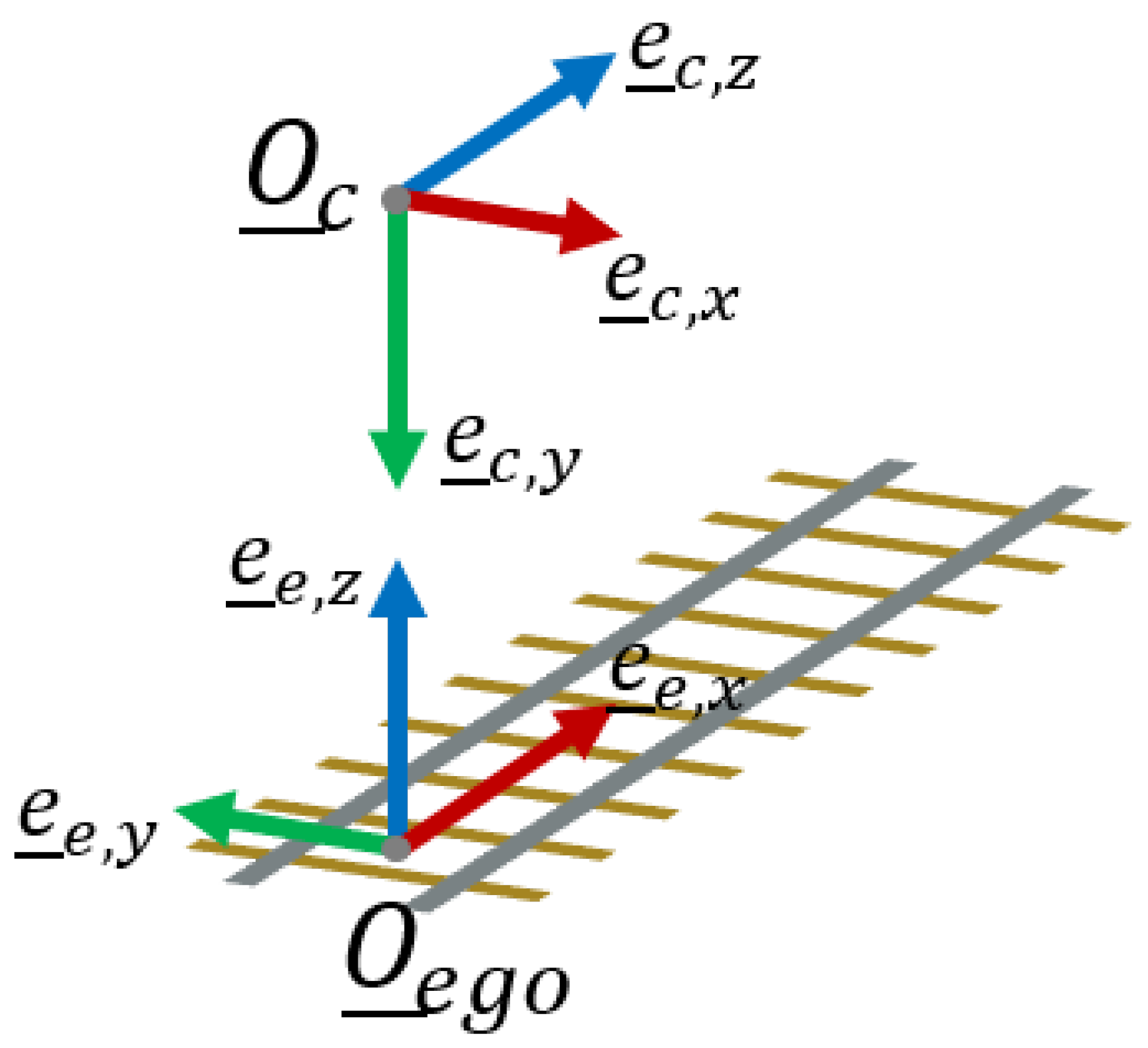
3. Methods

The pixelwise reprojection of an image into 3D space results in a point cloud ${\mathit{P}}_c$ represented in the camera’s coordinate system. In this coordinate system, the z-axis typically aligns with the optical axis, while the x- and y-axes correspond to the image dimensions. However, this setup poses challenges for tasks such as measuring the gauge of railway tracks, as the ground plane’s location remains undefined. Additionally, determining object heights or distances becomes problematic due to the pitch and roll of the camera.

In this section, we address these challenges by first detecting the rails in the image and projecting them into 3D space using a backbone depth prediction model. In the resulting 3D projection, we estimate the ground level and optimize the alignment of the detected rails to enable accurate gauge measurements. Furthermore, once the location and alignment of the rails are determined, we estimate the position of a more suitable coordinate frame, ${\underline{O}}_{ego}$, which aligns with the coordinate system defined in OSDaR23 and is illustrated in Figure 1.

3.1. Preliminaries

For proper functionality, we assume the camera to be positioned in the driver’s view, although it does not necessarily need to be mounted inside the driver’s cab. In fact, it can be installed anywhere at the front of the train. Additionally, we assume that the track on which the train is located (ego-track) is visible in the image. The intrinsic camera matrix is also required to be known. Finally, our approach assumes the train is either on a straight track or, at a minimum, a broad curve during the calibration process, as aligning the rails along a straight axis over a certain distance is essential for measuring the gauge.

3.2. Segmentation

The first step in our approach is to detect rails in the original image using a state-of-the-art image segmentation model. For this purpose, we select InternImage [32] as the most suitable model for our use case. According to [33], InternImage achieved the highest performance among models with a publicly available codebase and ranked second overall on the CityScapes dataset, with a mean Intersection over Union (IoU) of $84.1$, close behind VLTSeg with $84.4$. We consider the CityScapes dataset, which provides outdoor images from the automotive domain, as sufficiently similar to the railway domain.

InternImage is an encoder architecture that replaces standard convolutions with deformable convolutions, followed by a feed-forward network at each layer, enabling dynamic adaptation of receptive fields. This design yields a flexible, transformer-like architecture while preserving the locality and computational efficiency of convolutional operations. The authors implemented various decoding methods for both image classification and segmentation tasks. In this work, we adopt UPerNet [34] as the decoder, a segmentation-specific architecture that fuses multi-scale features via a Feature Pyramid Network and captures global context through a Pyramid Pooling Module, before upsampling and combining the features to generate dense, pixelwise predictions. Within the InternImage pipeline, UPerNet demonstrated strong performance on the CityScapes dataset.

However, as no pretrained InternImage model includes a class for rails, transfer learning is necessary. To accomplish this, we use the RailSem19 dataset [35], which contains 8500 unique images from the railway domain captured in driver’s view with additional semantic segmentations, including a class for rails (rail-raised). Since InternImage is built on top of the MMSegmentation [36] pipeline, we integrate RailSem19 into this framework and initially train the model using Cityscapes-pretrained weights, yielding a final mean IoU of $70.03$.

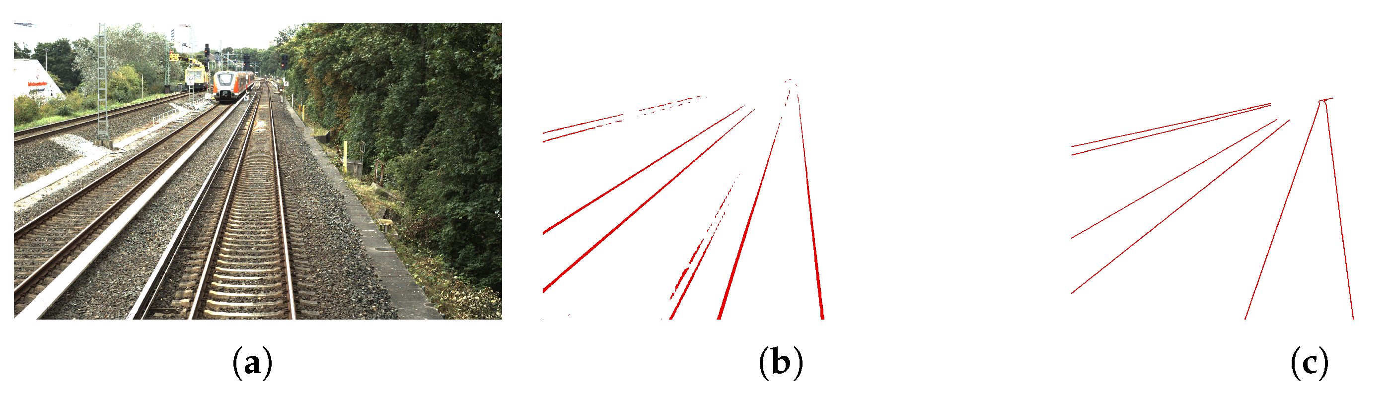
To evaluate the overall impact of the segmentation on the calibration accuracy, we additionally create ground truth segmentations for the OSDaR23 dataset. Although OSDaR23 does not directly provide ground truth segmentations, it includes polylines representing the rails. We leverage these polylines to generate ground truth segmentations by rasterizing them into images. Figure 2 provides an example of the segmentation results. To assess the robustness of our system on entirely unseen data, we explicitly train InternImage exclusively on the RailSem19 dataset and do not use our generated ground truths from OSDaR23 for training.

By applying segmentation, we assign a label to each pixel, and consequently to each corresponding 3D point. The set of all N 3D points labeled as rail-raised is defined as ${\mathit{P}}_d^r$, with dimensions $3\times N$. For images in the OSDaR23 dataset, this typically results in dimensions of approximately $3\times 7·{10}^6$.

3.3. Calibration

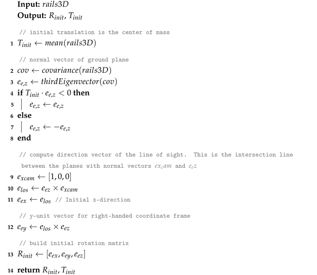
3.3.1. Estimating the Ground Level

Following the segmentation step, we determine the ground level, which we define as the plane perpendicular to the direction of least variance within ${\mathit{P}}_d^r$. To achieve this, we compute the normal vector of the ground plane as the third eigenvector of the covariance matrix of ${\mathit{P}}_d^r$. This normal vector is then assigned as the z-directional vector, ${\underline{e}}_{e,z}$, of the ego coordinate system:

$$\begin{array}{cc}\hfill {\underline{M}}_d^r& =mea{n}_{rw}\left({\mathit{P}}_d^r\right),\hfill \end{array}$$

(1)

$$\begin{array}{cc}\hfill {\mathit{P}}_d^{r^{\prime }}& ={\mathit{P}}_d^r-{\underline{M}}_d^r·{\mathbf{J}}_{1,N},\hfill \end{array}$$

(2)

$$\begin{array}{cc}\hfill {\underline{e}}_{e,z}& ={\nu }_3\{{\mathit{P}}_d^{r^{\prime }}·{\left({\mathit{P}}_d^{r^{\prime }}\right)}^T\}.\hfill \end{array}$$

(3)

Here ${\underline{M}}_d^r$ represents the row-wise mean and thus the center of mass of ${\mathit{P}}_d^r$. In Equation (2), ${\mathbf{J}}_{1,N}$ represents a matrix of ones with dimensions $1\times N$, ensuring that ${\mathit{P}}_d^{r^{\prime }}$ is mean-free. ${\nu }_3\left\{\mathit{x}\right\}$ denotes the third eigenvector of a matrix $\mathit{x}$.

This computation is ambiguous because it does not determine whether the eigenvector points upwards or downwards. To ensure that ${\underline{e}}_{e,z}$ points upwards, we verify its direction relative to the camera’s origin. Since we are working in camera coordinates, ${\underline{M}}_d^r$ can also be interpreted as a vector pointing from the camera’s origin to the center of mass of ${\mathit{P}}_d^r$. Given that the camera is naturally positioned above the rails, ${\underline{M}}_d^r$ must point downwards. Therefore, ${\underline{e}}_{e,z}$ should point in the opposite direction. This is ensured using the following computation:

$$\begin{array}{cc}\hfill {\underline{e}}_{e,z}& :={\underline{e}}_{e,z}\mathrm{if}{\underline{M}}_d^r·{\underline{e}}_{e,z}<0\mathrm{else}-{\underline{e}}_{e,z}.\hfill \end{array}$$

(4)

3.3.2. Estimating the Forward Direction

Once ${\underline{e}}_{e,z}$ is determined, the next step is to compute the corresponding x-directional vector ${\underline{e}}_{e,x}$. This vector is defined to align with the direction of the rails (see Figure 1). Its determination involves two stages: first, estimating the direction approximately using the Line of Sight (LoS), and second, refining it to ensure ${\underline{e}}_{e,x}$ runs precisely parallel to the rails.

First, we estimate the LoS, which we define as the primary direction the camera is oriented along at ground level. This direction corresponds to the line of intersection between the camera’s $y,z$-plane and the ground-level plane. Its directional vector ${\underline{e}}_{los}$ can be computed as follows:

$$\begin{array}{cc}\hfill {\underline{e}}_{los}& ={\underline{e}}_{e,z}\times {\underline{e}}_{c,x}.\hfill \end{array}$$

(5)

In camera coordinates, the camera’s unit vector in the x-direction is ${\underline{e}}_{c,x}={[1,0,0]}^T$. It is important to note that ${\underline{e}}_{los}$ does not necessarily align with the rails, as the camera is usually angled relative to the rail direction. However, assuming the camera is mounted in the driver’s view, ${\underline{e}}_{los}$ is expected to be approximately parallel to the rails. To accurately align the x-directional vector, we optimize the rotation of ${\underline{e}}_{los}$ around the ${\underline{e}}_{e,z}$-axis so that the resulting x-axis lies precisely parallel to the rails. For this, we define the initial x- and y-directional vectors of the ego coordinate system as:

$$\begin{array}{c}\hfill {\underline{e}}_{e,x}^{init}={\underline{e}}_{los},{\underline{e}}_{e,y}^{init}={\underline{e}}_{los}\times {\underline{e}}_{e,z}.\end{array}$$

(6)

The algorithmic process for this initial step of estimating the ego coordinate system is presented in Appendix A, Algorithm A2.

Next, we project ${\mathit{P}}_d^{r^{\prime }}$ onto the ground plane:

$$\begin{array}{cc}\hfill {\underline{k}}^T& ={\displaystyle \frac{{\underline{e}}_{e,z}^T}{{∥e_{e,z}∥}_2^2}}·\left({\underline{M}}_d^r·{\mathbf{J}}_{1,N}-{\mathit{P}}_d^{r^{\prime }}\right),\hfill \end{array}$$

(7)

$$\begin{array}{cc}\hfill {\mathit{P}}_g^{r^{\prime }}& ={\mathit{P}}_d^{r^{\prime }}+{\underline{e}}_{e,z}·{\underline{k}}^T,\hfill \end{array}$$

(8)

$$\begin{array}{cc}\hfill {\underline{P}}_{g,x}^r& ={\left[{\left({\underline{e}}_{e,x}^{init}\right)}^T·{\mathit{P}}_g^{r^{\prime }}\right]}^T,\hfill \end{array}$$

(9)

$$\begin{array}{cc}\hfill {\underline{P}}_{g,y}^r& ={\left[{\left({\underline{e}}_{e,y}^{init}\right)}^T·{\mathit{P}}_g^{r^{\prime }}\right]}^T,\hfill \end{array}$$

(10)

$$\begin{array}{cc}\hfill {\mathit{P}}_g^r& ={\left\{{\underline{P}}_{g,x}^r,{\underline{P}}_{g,y}^r\right\}}^T.\hfill \end{array}$$

(11)

All projected points, ${\mathit{P}}_g^r$, are now in 2D within the ground-level coordinate system. This coordinate system has its origin at ${\underline{M}}_d^r$, with the x-axis aligned along ${\underline{e}}_{los}$. To refine the alignment, we rotate all points ${\mathit{P}}_g^r$ around their center of mass until the rails are optimally parallel to the x-axis. The optimization objective is based on the histogram of the distribution of the y-coordinates. When the rails are perfectly aligned with the x-axis, the histogram exhibits the maximum deviation from a uniform distribution, as illustrated in Figure 3. Conversely, if the rails are perpendicular to the x-axis, the histogram approaches a uniform distribution.

To quantify the alignment, we use the chi-square test against a uniform distribution as the optimization objective:

$$\begin{array}{cc}\hfill {\chi }^2& =\sum _{j=1}^n{\displaystyle \frac{{(n_j-n_{0,j})}^2}{n_{0,j}}},\hfill \end{array}$$

(12)

where $n_j$ represents the observed frequency of the j-th bin, and $n_{0,j}$ is the expected frequency of the j-th bin. Since we are testing against a uniform distribution, the expected frequency is equal for all bins:

$$\begin{array}{cc}\hfill n_{0,j}& ={\displaystyle \frac{n}{n_{bins}}},\hfill \end{array}$$

(13)

where n denotes the total number of elements in ${\underline{P}}_{g,y}^r$. The bin width $b_w$ and number of bins $n_{bins}$ are estimated using the Freedman–Diaconis rule:

$$\begin{array}{cc}\hfill b_w& =2{\displaystyle \frac{IQR\left({\underline{P}}_{g,y}^r\right)}{\sqrt[3]{n}}},\hfill \end{array}$$

(14)

where $IQR\left({\underline{P}}_{g,y}^r\right)$ is the interquartile range of the samples in ${\underline{P}}_{g,y}^r$, representing the interval containing the middle 50 % of the points. The number of bins is then calculated as:

$$\begin{array}{cc}\hfill n_{bins}& ={\displaystyle \frac{max\left({\underline{P}}_{g,y}^r\right)-min\left({\underline{P}}_{g,y}^r\right)}{b_w}}.\hfill \end{array}$$

(15)

We optimize the rotational angle $\alpha$ using various algorithms, including brute force optimization, which is computationally feasible in this context. The resulting optimized angle, $\widehat{\alpha }$, is then applied to rotate all points in ${\mathit{P}}_g^r$, ensuring that the rails are optimally aligned parallel to the ego-track.

The algorithmic process for this optimization step is presented in Appendix A, Algorithm A4.

3.3.3. Estimating the Scale

We now analyze the optimized histogram illustrated in Figure 4. The narrow peaks in this histogram correspond to the rails. Our goal is to measure the distance between the two rails of the ego-track. To achieve this, we first group the clusters in the histogram using the DBSCAN algorithm [37] and identify those representing the rails of the ego-track. Given that the camera is mounted on the ego-train, it is positioned close to the ego-track in the ego y-coordinate. Leveraging this information, we identify the two cluster centers closest to the LoS y-coordinate at the camera’s position, projected onto the ground plane. These cluster centers are designated as the ego-rails, with y-coordinates $y_l^{er}$ for the left rail and $y_r^{er}$ for the right rail.

The final scaling factor is then computed based on the distance between $y_l^{er}$ and $y_r^{er}$, ensuring that this distance matches the known track gauge, ${\Delta }_g$:

$$\begin{array}{cc}\hfill s& ={\displaystyle \frac{{\Delta }_g}{y_l^{er}-y_r^{er}}}.\hfill \end{array}$$

(16)

Using this scaling factor, we can now convert an unscaled point cloud ${\mathit{P}}_c$ to a metric-scaled point cloud ${\mathit{P}}_{c,m}$:

$$\begin{array}{cc}\hfill {\mathit{P}}_{c,m}& =s·{\mathit{P}}_c.\hfill \end{array}$$

(17)

3.3.4. Estimating the Extrinsic Calibration

After scaling the point cloud, we can utilize the fact that an ego coordinate system is now computable, with directional vectors oriented upwards and along the rails (see Figure 1). First, we compute the optimized directional x- and y-vectors as:

$$\begin{array}{cc}\hfill {\underline{e}}_{e,x}& =\mathit{R}(0,0,\widehat{\alpha })·{\underline{e}}_{e,x}^{init},\hfill \end{array}$$

(18)

$$\begin{array}{cc}\hfill {\underline{e}}_{e,y}& ={\underline{e}}_{e,x}\times {\underline{e}}_{e,z},\hfill \end{array}$$

(19)

where $\mathit{R}(0,0,\widehat{\alpha })$ is the rotational matrix with zero roll and pitch, and $\widehat{\alpha }$ is the yaw angle. With these conditions, we have established a right-handed coordinate system. However, up to this point, we have only determined the directional vectors of this system. The origin lies at ${\underline{M}}_d^r$, which is not ideal, as ${\underline{M}}_d^r$ can vary between consecutive frames. Therefore, we shift the origin to a more practical location, as illustrated in Figure 5.

Given that we already know the y-coordinates of the ego-rails, we position the origin between these rails and below the camera. The new origin is thus defined as:

$$\begin{array}{cc}\hfill {\underline{O}}_{ego}& =\left[\begin{array}{c}{x}^{cam}\\ y_l^{er}+0.5·(y_r^{er}-y_l^{er})\\ 0\end{array}\right].\hfill \end{array}$$

(20)

Please note that this formula applies only before the point cloud is scaled. If the point cloud has been scaled, $y_l^{er}$ and $y_r^{er}$ must also be scaled before applying this formula. Here, $x^{cam}$ represents the x-coordinate of the camera’s origin in the ego coordinate system, where the origin is still located at ${\underline{M}}_d^r$. After shifting the origin to ${\underline{O}}_{ego}$, the resulting origin lies directly beneath the camera and at the center of the ego-track, as shown in Figure 5.

The algorithmic process for the scaling and extrinsic calibration step is presented in Appendix A, Algorithm A3, along with the complete pipeline described in Algorithm A1.

3.4. Hyperparameter Selection

Our algorithm includes the following hyperparameters: For models that predict pixelwise depth, a maximum depth threshold must be specified to determine which pixels are included. For models predicting pixelwise disparity, a minimum disparity threshold must be defined to select the relevant pixels. Additionally, parameters $ϵ$ and $n_{nb}$ need to be set for the DBSCAN algorithm, which is used to identify the rail positions in the histogram.

For the maximum depth, we choose 20 m, and for the minimum disparity, we select 15 pixels. Beyond these thresholds, the algorithm’s performance tends to degrade, as too few points are segmented as rail-raised.

In the DBSCAN algorithm, $ϵ$ represents the maximum distance between two points for them to be considered part of the same cluster, and $n_{nb}$ denotes the minimum number of points required for a cluster to be recognized. The choice of these hyperparameters is highly dependent on the characteristics of the point cloud, such as the number of points classified as rails and the overall scaling. To address this dependency, we decouple the parameters.

Since $n_{nb}$ specifies the number of points required for a cluster, we relate it to the total number of points in the point cloud. For $ϵ$, which defines the maximum distance between two points within a cluster, we aim to link it to the maximum distance between points in the cloud (i.e., the difference between the maximum and minimum values in ${\underline{P}}_{g,y}^r$). Although it would be ideal to relate $ϵ$ to the average distance between points, this would significantly increase computational effort. We address this by considering a maximum of 10 parallel rails visible as an edge case and hence set $ϵ$ to ${\displaystyle \frac{1}{10}}$ of the maximum distance in the point cloud and $n_{nb}$ to ${\displaystyle \frac{1}{10}}$ of the total number of points in the point cloud.

3.5. Evaluation

We evaluate our method on the OSDaR23 dataset [3], which provides LiDAR point clouds as ground truth. To the best of our knowledge, this is the only dataset suitable for this task, offering synchronized camera and LiDAR data from railway scenes, along with ground truth extrinsic calibrations. The dataset consists of 45 unique scenes with approximately 1600 images in total. From this, we identify 21 scenes containing approximately 870 recordings that meet the preliminary requirements (see Section 3.1) for every recording within the scene.

We assume LiDAR provides higher accuracy than camera due to its native 3D sensing, avoiding the inaccuracies caused by the camera’s reduction to 2D. To align with camera data, we remove LiDAR points outside the camera’s field of view and limit evaluations to a range of 50 m ahead of the train.

We use the Chamfer distance as the evaluation metric, which quantifies the discrepancy between two point clouds in a metric-based manner. Given the point cloud from our method ${\mathit{P}}_{c,m}$ with N points and the respective LiDAR point cloud ${\mathit{P}}_l$ with M points, the Chamfer distance is defined as:

$$\begin{array}{cc}\hfill CD\left({\mathit{P}}_{c,m},{\mathit{P}}_l\right)={\displaystyle \frac{1}{2}}·& \left({\displaystyle \frac{1}{N}}{\displaystyle \sum _{i=0}^N}{\left|x_i-NN\left(x_i,{\mathit{P}}_l\right)\right|}_2\right.\hfill \\ \hfill & +\left.{\displaystyle \frac{1}{M}}{\displaystyle \sum _{j=0}^M}{\left|x_j-NN\left(x_j,{\mathit{P}}_{c,m}\right)\right|}_2\right),\hfill \end{array}$$

(21)

where

$$\begin{array}{cc}\hfill NN\left(x,\mathit{P}\right)& =argmi{n}_{x^{\prime }\in \mathit{P}}{\left|x-x^{\prime }\right|}_2.\hfill \end{array}$$

(22)

To meet legal requirements for vegetation clearance, we aim for an average Chamfer distance below 1 m.

4. Experimental Results

We evaluate our method in three stages. First, we assess the scaling process without applying extrinsic calibration to enable comparison with an existing benchmark. In this stage, we transform between LiDAR and camera coordinates using the parameters provided in the dataset for both the benchmark and the scaled point clouds. Next, we evaluate the extrinsic calibration, setting a benchmark for estimating OSDaR23-specific extrinsics using only a single image. Finally, we analyze the accuracy of the scaled and extrinsically calibrated 3D point clouds to determine the overall performance of our approach. It is important to note that while the first stage can be compared against an established benchmark, no benchmark currently exists for extrinsic calibration to the OSDaR23-specific coordinate system.

4.1. Evaluation of the Scaling

We start by establishing a benchmark. We evaluate four recently published models that predict metric depth and are at least partially designed for outdoor scenes. These include the most recent models, UniDepth [2] (2025) and Depth Pro [21] (2024), as well as Depth Anything [20] (2024) and AdaBins [38] (2021). For UniDepth, we evaluate both the depth prediction model and the point cloud prediction model (UniDepth Points). For each recording in the dataset, we calculate the Chamfer distance, averaging first scene-wise and then across the entire dataset. The results are presented in Figure 6.

UniDepth and Depth Pro significantly outperform Depth Anything and AdaBins across all scenes, while demonstrating comparable performance to each other. Overall, UniDepth achieves the lowest average Chamfer distance and is therefore adopted as our benchmark model. It is worth noting that with an average Chamfer distance of $1.94$ m across the entire dataset, the reconstruction using UniDepth is still inadequate for the current use case.

We now evaluate the scaling using three backbone depth prediction models. The first model, UniDepth, aligns with our benchmark as it is the most recent depth prediction model. This allows us to assess the potential improvement in reconstruction accuracy achieved through our calibration. The second model, DepthPro [21], demonstrates performance comparable to UniDepth and is therefore included in our evaluations. Finally, the third model, MiDaS [19], predicts disparities and hence provides relative depth. By applying our calibration, we convert MiDaS outputs into metric space and evaluate their accuracy. It is important to note that for the rail gauge measurement, the backbone model must predict rails as parallel structures in the resulting 3D point cloud. This criterion is met by all selected models, but is not sufficiently satisfied by Depth Anything or AdaBins.

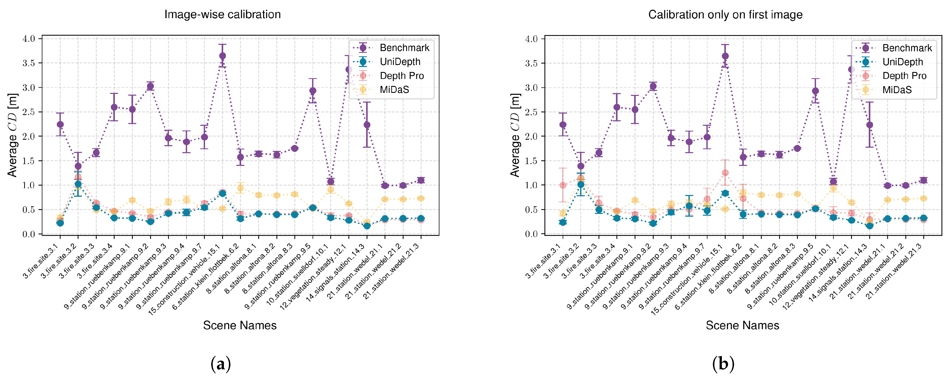
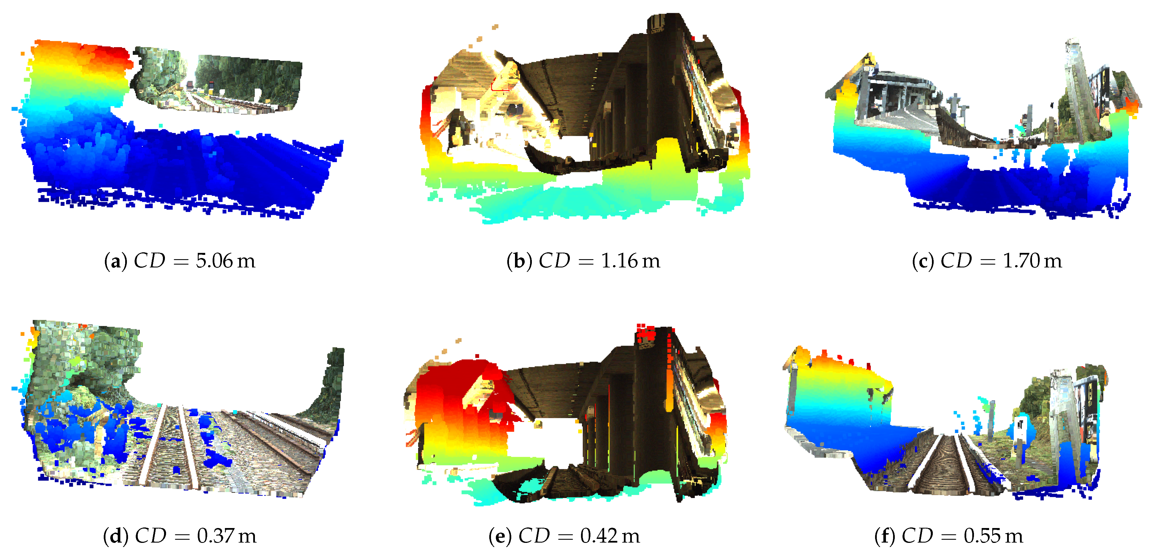
For each recording that matches the preliminaries, we perform calibration using InternImage segmentation. The results are then compared against the benchmark. Figure 7a illustrates the results. Our calibration method significantly reduces the average Chamfer distance using all backbones. Furthermore, Figure 7a demonstrates consistent improvements across all scenes. The averaged results are presented in

Table 1. Summary of the experimental results on scaling.

Experiment	Average Chamfer Distance
	Benchmark	Result
		UniDepth	Depth Pro	MiDaS
Image-wise calibration	$2.01$ m	0.41 m	$0.46$ m	$0.65$ m
First image calibration	$2.01$ m	0.42 m	$0.55$ m	$0.65$ m
Average calibration	$1.94$ m	0.71 m	$1.15$ m	$0.89$ m

. Additionally, the visual examples in Figure 8 demonstrate that scaling significantly enhances the reconstruction quality compared to LiDAR.

Generally, it would be advantageous if calibration did not need to be performed for every single recording. In practice, there are scenarios where our preliminary conditions are not met, so being able to calibrate only when these conditions are satisfied and then apply the calibration to other recordings would be highly beneficial.

Given consistent intrinsic and extrinsic camera parameters across the dataset, this approach is feasible. However, dynamic factors such as auto white balance or contrast adjustments under varying lighting conditions (e.g., brighter or darker scenes) could still affect depth prediction and result in scale variations, as illustrated in Figure 8. To assess the impact of omitting individual calibration in stable ambient conditions, we calibrate only the first recording of each scene and apply this calibration to all subsequent recordings within the same scene. Figure 7b presents the results, demonstrating again improved reconstructions across all scenes. The averaged results are presented in Table 1.

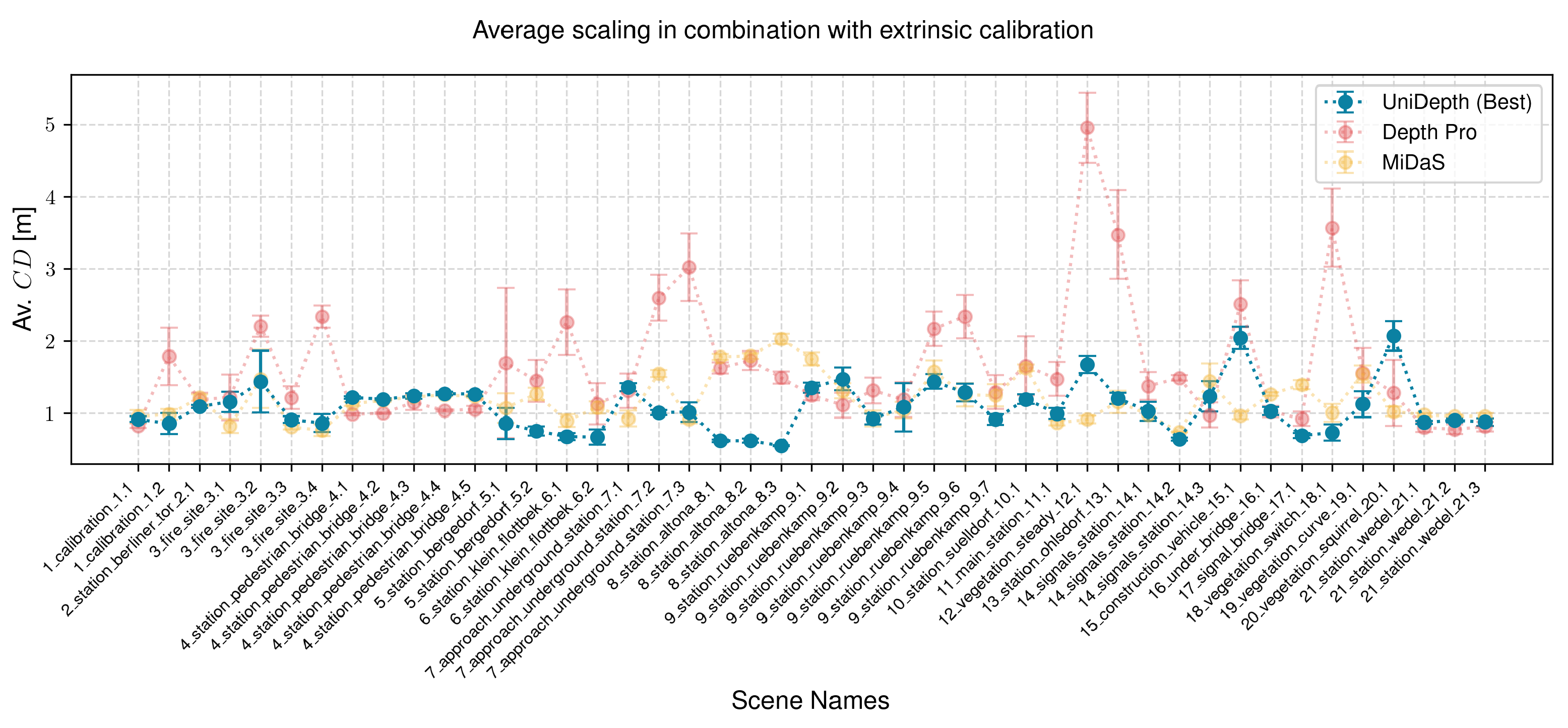
There are 24 scenes in the dataset that do not meet the preliminary requirements. These scenes often feature significantly different ambient conditions, such as transitions between overground and underground environments, which affect the scaling of the depth prediction backbone. To evaluate this effect, we average the calibration parameters from all scenes meeting the preliminary criteria and apply this averaged calibration to the entire dataset.

The results, presented in Figure 9, indicate that when using UniDepth (Best) as the backbone, the average Chamfer distance improved significantly across all scenes except one (2%). The scene 7_approach_underground_station_7.1 exhibited a slight deterioration of $0.13$ m. Despite this, the reconstruction in that scene remained meaningful, and both Depth Pro and MiDaS backbones achieved improvements in this scene. Using Depth Pro, six scenes (13%) showed no improvement, while MiDaS failed to improve five scenes (11%).

These results demonstrate that even in this challenging case, UniDepth exhibited only minimal degradation (2%, $0.13$ m), while achieving a substantial overall improvement in reconstruction accuracy, from an average Chamfer distance of $1.94$ m without calibration to $0.71$ m with calibration. Furthermore, as illustrated in Figure 7a,b, all scenes that failed to improve in this experiment using Depth Pro or MiDaS backbones had previously shown improvements under both image-wise and initial calibration methods. This suggests that regular updates to the calibration during operation will consistently yield improvements, even if calibration is not performed for every single recording. Averaged results are presented in Table 1.

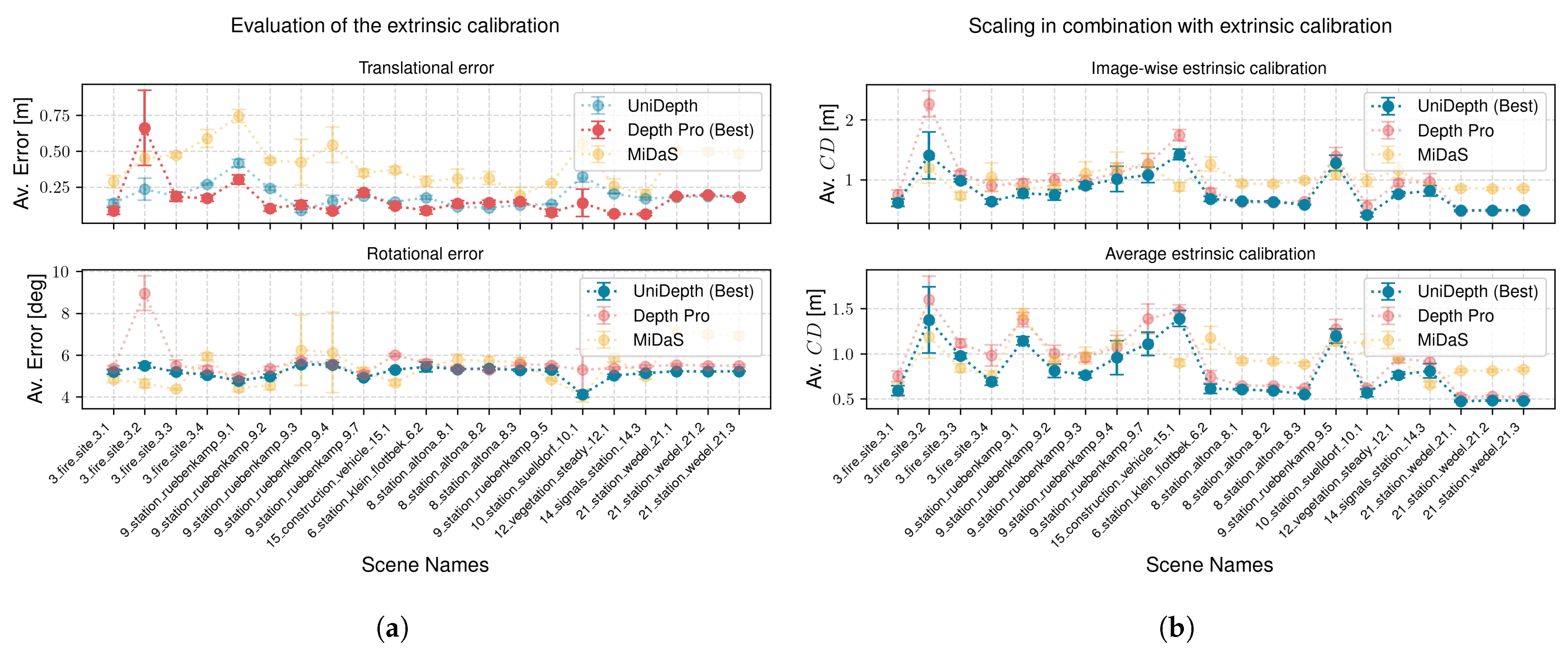
4.2. Evaluation of the Extrinsic Calibration

We proceed to evaluate the extrinsic calibration by considering all scenes that meet the preliminary conditions. The calibration is performed image-wise and evaluated separately for translation and rotation. For each case, we compute the average $L2$-norm relative to the ground truth provided in the dataset. To evaluate rotation, the given quaternion is converted into Euler angles for comparison. The results are presented in Figure 10a.

Table 2. Average deviations of extrinsic calibration parameters from ground truth.

Parameter	Average Error
	UniDepth	Depth Pro	MiDaS
Translation	$0.19$ m	0.16 m	$0.41$ m
Rotation	5.17 deg	$5.61$ deg	$5.45$ deg

presents the deviation of the final averaged extrinsic parameters.

4.3. Evaluation of Scale in Combination with Extrinsic Calibration

We evaluate the accuracy of combining scaling with extrinsic calibration to better understand the impact of errors in the extrinsic calibration. First, we scale the point cloud and transform it into the ego-coordinate frame using our estimated extrinsic calibration. The results are then compared with LiDAR point clouds, transformed using the ground truth extrinsics from the OSDaR23 dataset.

As in Section 4.1, we start by evaluating image-wise scaling and image-wise extrinsic calibration across all scenes that meet the preliminary requirements. The results are shown in the upper subplot of Figure 10b. Unlike the scale factor, extrinsic calibration is a fixed physical setup unaffected by dynamic camera parameters. Therefore, in the next experiment, we average the extrinsic calibration and apply it to the image-wise scaled point clouds. This represents an operational scenario where extrinsics are consistently averaged while scaling remains dynamic. The results of this approach are shown in the lower subplot of Figure 10b.

Finally, we evaluate using an averaged scale and averaged extrinsic calibration across the entire dataset. The results are presented in Figure 11. The average Chamfer distances for all three experiments are additionally summarized in

Table 3. Summary of the experimental results on scaling combined with extrinsic calibration.

Experiment	Average Chamfer Distance
	UniDepth	Depth Pro	MiDaS
Pure Image-wise	0.80 m	$0.95$ m	$0.98$ m
Av. extr. Image-wise scale	0.81 m	$0.94$ m	$0.96$ m
Average Extr. and Scale	1.08 m	$1.64$ m	$1.19$ m

.

4.4. Additional Experiments

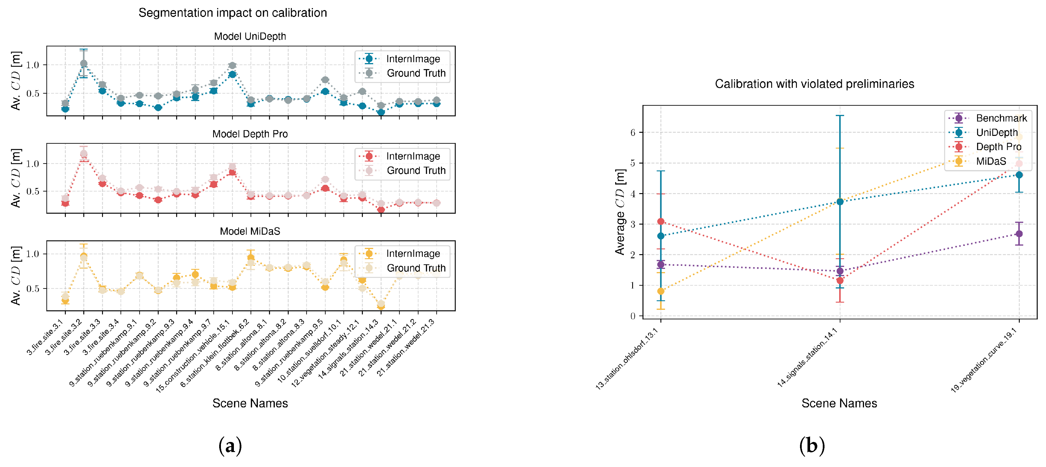
4.4.1. Impact of the Segmentation Accuracy

In addition to our evaluation experiments, we aim to assess the impact of segmentation accuracy on calibration quality. To achieve this, we calibrate and evaluate our system again using the ground truth segmentation data we created (see Section 3.2). Evaluations are performed image-wise across all scenes meeting the preliminary criteria, with results presented in Figure 12a.

The comparison reveals no significant advantage of using ground truth over the InternImage segmentation. Quantitative analysis shows an average Chamfer distance of $0.51$ m (ground truth) versus $0.41$ m (InternImage) with the UniDepth backbone, $0.53$ m (ground truth) versus $0.46$ m (InternImage) with the Depth Pro backbone, and $0.64$ m (ground truth) versus $0.65$ m (InternImage) with the MiDaS backbone. These results suggest that calibration using ground truth segmentation can sometimes yield poorer outcomes than using InternImage. A possible explanation is that segmentation by a model like InternImage may act as a natural low-pass filter, mitigating the effects of inaccuracies by excluding challenging parts of the image through missed classifications, thereby improving overall depth prediction.

4.4.2. Calibration with Violated Preliminaries

Additionally, we aim to assess the impact of calibrating recordings in scenarios where the preliminary requirements are significantly violated. We identify three cases characterized by different types of violations. The first case involves a train positioned directly in front of a switch, where the ego-track is not yet intersected by the merging track (13_station_ohlsdorf_13.1). In the second case, the train is located on a switch, where the ego-track is intersected by the merging track (14_signals_station_14.1). In the third case, the train is located on a narrow curve (19_vegetation_curve_19.1).

Figure 12b and

Table 4. Average Chamfer distances obtained from calibration under significantly violated preliminary conditions.

Scene	Average Chamfer Distance
	Benchmark	Result
		UniDepth	Depth Pro	MiDaS
13_station_ohlsdorf_13.1	$1.68$ m	$2.62$ m	$3.09$ m	0.81 m
14_signals_station_14.1	$1.46$ m	$3.73$ m	1.16 m	$3.75$ m
19_vegetation_curve_19.1	2.68 m	$4.61$ m	$4.98$ m	$5.85$ m
Average	1.94 m	$3.65$ m	$3.07$ m	$3.47$ m

present the results of these scenarios. The analysis reveals that whether the result is improved or deteriorated depends heavily on the type of violation and the backbone model used. This variability suggests that the behavior of calibration under violated preliminary conditions cannot be consistently defined.

5. Summary and Discussion

This study presents a novel approach for scaling non-metric 3D point clouds using monocular depth or disparity estimation, combined with achieving extrinsic camera calibration from a single image in the railway context. As demonstrated, direct metric estimation using neural networks fails in achieving the accuracy required to reliably assess vegetation encroachment into the structural gauge. To address this, we developed a method for scale estimation and extended it to compute reliable extrinsic calibration.

The proposed method is based on high-quality rail segmentation. By adapting the InternImage segmentation model, pretrained on the CityScapes dataset, to the Railsem19 dataset, we achieve rail segmentation that delivers scaling performance comparable to using ground truth segmentation. This segmentation enables scale estimation by measuring the rail gauge in the point cloud and aligning it with the standard European gauge of $1.435$ m. Additionally, the point cloud is rotated to align the rails with the x-axis and detect the ego-track, enabling precise extrinsic calibration from a single image.

Our evaluation shows that the method reduces the average Chamfer distance from the benchmark value of $2.01$ $\mathrm{m}$ to $0.41$ $\mathrm{m}$, when the preliminary conditions are met. Even when calibration is performed only at the beginning of a scene, the Chamfer distance remains low at $0.42$ $\mathrm{m}$. In both scenarios, our method outperforms the benchmark across all evaluated scenes. When environmental conditions vary significantly, such as transitioning between outdoor and underground environments, and the scaling factor is averaged, the method achieves a Chamfer distance of $0.71$ $\mathrm{m}$. Although one scene (2%) in this challenging case did not outperform the benchmark, the deterioration was low ($0.13$ m), and the overall reconstruction quality remained high. Additionally, in this context, we demonstrated that both Depth Pro and MiDaS backbones outperformed the benchmark in this particular scene, and that individual scaling outperformed the benchmark in all scenes where these backbones exhibited deterioration.

The system computes extrinsic calibration with an average error of $0.16$ $\mathrm{m}$ and $5.17$°, aligning the scaled point cloud with a coordinate system that facilitates structural gauge inspection by closely resembling real-world spatial dimensions. In this system, equivalent to OSDaR23, the ground lies in the x-y plane, the x-axis aligns with the direction of motion, and the z-axis represents height, similar to the center-rear-axis coordinate frame used in the automotive domain. To the best of our knowledge, no extrinsic calibration method has been published that aligns with this coordinate system and relies solely on single monocular images without additional sensors, making this approach a new benchmark in the field. Transforming the scaled point cloud into this coordinate system yields an average Chamfer distance of $0.80$ $\mathrm{m}$, when averaging the scale factor across all environmental conditions, of $1.08$ $\mathrm{m}$.

The method can be implemented using a mobile camera or smartphone to monitor structural gauge violations. Referring to the ego-track, preliminary conditions can be verified, i.e., using [39]. Continuous scaling estimation under fulfilled preliminary conditions ensures system robustness, while extrinsic calibration can be consistently averaged over time. In contrast, scaling factor averaging across varied conditions may be insufficient, emphasizing the importance of on-demand scale estimation for accuracy. This setup provides a foundation for early detection of vegetation encroachment into the structural gauge, meeting the German legal requirement of a 1 m clearance besides the structural gauge, and demonstrating its practical applicability.

Future research in this field should explore the application of the method in real-time scenarios. While real-time processing is not required for the current use case, as data can be post-processed or handled via a cloud application, it would still be valuable to investigate time requirements and performance under real-time constraints. To further refine the scaling factor, future studies could evaluate improvements by incorporating data from neighboring tracks, when available. Additionally, accuracy could potentially be enhanced by investigating the effects of camera orientation errors and changing weather conditions, as these factors can significantly influence system reliability in operational environments. To strengthen the method further, registering multiple consecutive images and leveraging additional sensors such as IMUs or GPS could enable more robust scene registration. This approach would be particularly beneficial for improving the accuracy of extrinsic calibration.