The Analysis of the Possibility to Conduct Orbital Manoeuvres of Nanosatellites in the Context of the Maximisation of a Specific Operational Task

Abstract

Satellite imaging has become very popular in recent years. Nanosatellites have been attracting growing interest as they proved to be a good alternative for the realisation of missions with the aim to monitor the environment from space and to acquire image data from every place on Earth. In spite of the short revisit time that is achieved by existing satellite constellations, a method was developed for the digital determination of the orbital manoeuvres for single nanosatellites. The aim of the analysis was to study the possibilities of the optimisation of orbital operations in the context of maximising the operational efficiency of the mission. The conducted experiments involved the assessment of various scenarios of orbital manoeuvres taking into consideration the key limitations, such as the available fuel weight, propulsion efficiency, and the requirements concerning time and energy. The obtained results revealed that the most efficient manoeuvres are those that balance the minimum consumption of fuel or energy with the maximum extension of the duration of the satellite’s stay above the area of interest. For example, slight adjustments to the altitude of the orbit with the use of Hohmann transfer proved to be optimal in terms of fuel costs. On the other hand, changes in inclination, although they are definitely energy-consuming, may significantly improve the coverage of the defined area. The conclusions from the conducted analyses confirmed that an appropriate strategy of orbital manoeuvres may greatly improve the operational efficiency of the nanosatellite, while, at the same time, continuing to save fuel and energy. It is suggested that future research should develop towards more advanced optimisation techniques, such as artificial intelligence algorithms that may additionally improve the precision and efficiency of planning orbital trajectories.

1. Introduction

Satellite imaging is one of the most dynamically developing areas of application of space technologies. Earth observation satellite systems may acquire images via remote sensing sensors [1]. Due to their multiple advantages, including the ability to capture image data from any place on Earth, regardless of the atmospheric conditions and time of the day, the ability to observe vast areas of land, as well as the short revisit time, remote sensing satellites are used in environmental monitoring, spatial planning, supporting crisis management activities, and supporting national defence and security. In the twenty-first century, the small satellite technology has played an important role in the development of space technologies. Significant technological progress was observed in the field of small satellites, weighing from 1 to 500 kg. One of the classes of the small satellite category is the NanoSat-class (1–10 kg). Nanosatellites were generally used to test, experiment with, and analyse new space equipment or software together with new concepts, at a minimum cost [1]. Although the number of imaging satellites continues to grow, there are still some limitations that prevent the fulfilment of all requirements of the users [2]. Such an example may be the early detection of fires. In this case, images must be acquired as often as possible so that the information about new fire outbreaks is provided as early as possible. Imaging satellites in their regular orbits are unable to observe the given area at the required time [2] and in the desired resolution. Due to that, in such a case, the satellite has to be transferred to a new orbit that will allow it to achieve high-resolution data, larger terrain coverage, and a short time of revisit. This issue is referred to as the orbit optimisation problem. It has been long known that the relation between the lifespan of a satellite and the altitude of its orbit depends on several factors. These include limitations resulting from atmospheric drag, factors related to radiation, such as high-energy particles, damage caused by micrometeoroids, atomic oxygen (AO), and ultraviolet (UV) radiation. In particular, the harsh conditions prevailing in low Earth orbit (LEO) can lead to complex, mutually reinforcing surface and satellite system degradation processes. Therefore, when considering orbit optimisation, a thorough assessment of these environmental conditions should be conducted, especially in the context of extending the operational lifespan of a nanosatellite [3]. However, the limitations for circular and elliptical orbits are slightly different. All spaceports are constructed in the vicinity of the equator (as close to the equator as possible for the given country), so that the rockets that are launched to the east gain some free velocity as a result of the Earth’s rotation. Equatorial space ports offer the possibility to achieve a high inclination (the angle of inclination of the orbital plane to the equatorial plane) [4]. Defining a specific orbit and conducting the orbit manoeuvres for satellites are extremely important problems in the science of orbital mechanics. As a result, the issue of transferring a spacecraft between orbits has been gaining increasing attention in recent years [5]. Many important problems in astrodynamics are related to the modification of the satellite’s orbit in order to achieve a specific trajectory for the planned space mission [6]. The aim of orbit manoeuvres is to transfer the spacecraft from one orbit to another. Such manoeuvres may be radical, for example transferring the satellite from a low parking orbit to inter-planetary trajectory. However, they may also be small, like at the last stages of the meeting of two spacecrafts. Changing the orbit requires launching the rocket engines [7], e.g., by applying a short impulse. The speed and inclination of the satellite may be modified by the rocket engine thrust that is specifically directed and lasts as long as it is necessary to achieve the desired result. The manoeuvre should be conducted at the right moment. In the atypical conditions of an orbital flight, the movement is different from the one that we are used to on Earth’s surface (and even in the air or on the orbit). A rocket engine is extremely powerful and works for very short periods, so that the change in the orbital velocity is, in fact, instantaneous. In general, the issue of optimisation of orbit manoeuvres may be discussed as a type of orbit design problem [8,9,10]. For many years, a great number of studies have been conducted with the aim to analyse the issues related to orbit design. For example, Graham et al. [11] analysed the problem of the determination of the minimum manoeuvring duration on an Earth orbit with the use of a low-thrust engine during an eclipse with great accuracy. The problem of changing the orbit was presented as a multi-phase optimum control issue, in which the spacecraft may only be propelled during those phases when the Sun remains within its reach. A method was developed to generate the initial assumptions in order to create the appropriate approximation. Then, the approximate locations where the spacecraft exits and enters Earth’s shadow were analysed. A similar issue was discussed by Zhang et al. [12]. In their article, the authors presented the problem of optimising the minimum fuel consumption for low-thrust propulsion in the context of orbit manoeuvres using three bodies of a limited weight. On the other hand, Wang et al. [13] presented a numerical convex optimisation method to solve the problem of an orbit manoeuvre conducted in the minimum time with the use of low thrust. Considering the uncertainty of the application of the previous methods, Mohammadi et al. [14] proposed a new method for the optimisation of impulse orbit manoeuvres. This study combines genetic algorithm, Monte Carlo sampling, and a substitute model so as to enable optimisation at the maximum speed. At the same time, it provides the most efficient solutions possible that are free from limitations and enables reaching the appropriate balance between optimisation accuracy and its duration. In one of the most recent studies, Morante et al. [15] proposed an optimum trajectory for changing the altitude of the orbit, which takes into account chemical, electric, and hybrid propulsion systems. Cheng et al. [16] proposed an optimum approach to controlling a spacecraft in real time. This method employs deep learning technologies in order to achieve the optimum trajectory of the spacecraft with a solar sail in the minimum amount of time for the purposes of an orbit manoeuvre. However, a major part of the problems that are related to orbit design is solved by striving to achieve the optimum orbit to improve its efficiency (e.g., the time when the satellite is positioned above the target as well as fuel consumption) [8,9,17]. These studies assume that the satellite is moving constantly on a single orbit, without doing any orbit manoeuvres, and that the elements of the orbit are changeable. There are a few studies that consider the orbit manoeuvres that focus only on changing the position of satellite constellations. Orbital manoeuvres, as opposed to orbit adjustment manoeuvres, are seldom performed, and, apart from that, they require significant amounts of fuel to perform every single operation. The aim of the manoeuvres is to achieve the desired configuration of the constellation that will meet the requirements related to reach [18,19,20]. He et al. [21] developed a method of physical programming with a genetic algorithm to solve the multi-task problem of the configuration of a constellation of satellites for disaster monitoring. Wang et al. [22] proposed to eliminate the disadvantages of traditional methods, such as long computation time, which usually limit engineering applications, by an innovative optimisation method: an algorithm for hybrid-resampling particle swarm optimisation (HRPSO) that improves the efficiency of constellation design. The method takes into account various types of sensors, the manoeuvre of their position, and various range efficiency indicators. On the other hand, Soleymani et al. [23] presented a new method of configuration of orbital satellite constellations based on Lambert’s theorem. They emphasised that, due to the cost and risk reduction, it is essential to consider the problem of the reconfiguration of satellite constellation, with two limitations: minimisation of the overall mission costs and the desired final configuration. In order to meet the requirements in the monitoring of crisis situations, in a recent study, Hu et al. [24] proposed a solution in the form of a multi-task framework for the problem of the optimisation of a satellite constellation that will be suitable for satellite constellation designers to identify the key compromises and make decisions. Although the issue of orbital manoeuvre optimisation has already been addressed in the literature, these issues are still relatively rarely explored, particularly in the context of nanosatellites, which operate under significant resource constraints, such as limited fuel mass, restricted energy availability, or simplified propulsion systems. The literature is dominated by studies focused on classical satellites or comprehensive optimisations using advanced algorithms, while there is a lack of simple and comparative analyses of manoeuvres typical for NanoSat-class missions. This study attempts to solve the issue of the possibility to conduct orbital manoeuvres of nanosatellites in the context of the maximisation of a specific operational task. The satellite may change its orbit, by performing an impulsive manoeuvre in a specific time, which, in turn, affects the efficiency of the orbit. The determination of a well-conceived power and direction of the impulse, as well as the moment of performing the manoeuvre, are of fundamental importance. As opposed to most of the previous works, which were aimed at the determination of a promising position (i.e., elements of the orbit) of the satellite, this study focuses on maximising a defined operational task by performing an orbital manoeuvre by the nanosatellite. The authors of this paper focus only on impulsive manoeuvres, where rockets are launched in relatively short series to create the required change in velocity (∆v).

The main contribution of this research consists of conducting a detailed analysis of orbital manoeuvres of nanosatellites in terms of their fuel and energy efficiency. The analysis allowed for the identification of the optimal manoeuvring strategies that may contribute to improving the efficiency of satellite missions. Numerical experiments were conducted, including various operational scenarios, such as changes in the altitude, inclination of the orbit, and the tilt of the satellite platform, with the aim to assess the efficiency and the energy costs of manoeuvres in the context of their practical applications. The performed analyses revealed the following:

• Different types of orbital manoeuvres of nanosatellites differ significantly in terms of fuel consumption, depending on the scale of change in the required parameter. For example, the altitude change manoeuvre is characterised by relatively low fuel consumption when the impulses are precisely planned, but the consumption of fuel for additional orbital manoeuvres is significantly limited by performing regular orbit adjustments.
• Parameters, such as altitude, inclination, and the tilt of the satellite have a major influence on the fuel and energy requirements of the manoeuvres. The optimum strategies vary depending on the specific requirements of the given mission, such as the need for the precise coverage of target areas or to maintain the orbit for a longer period.
• Impulsive manoeuvres proved to be an effective method to modify the parameters of the orbit, enabling precise control over the trajectory with a minimum time required to perform the manoeuvre. However, the manoeuvre of tilting the nanosatellite, with the telescope, with the use of reaction wheels, enables to prolong the time of observation of a specific area without the need to consume fuel. In this case, the satellite uses the energy generated by solar panels, which significantly lowers operating costs and improves the flexibility of the mission.
• The research results may be used to improve the planning of nanosatellite missions, in particular, by identifying the manoeuvres that are the most cost-effective in terms of fuel and energy, which will allow to maximise their operational efficiency.
• Combining orbital manoeuvres (such as changing the altitude or inclination) with the satellite tilting manoeuvre ensures the best balance between fuel and energy efficiency and operational precision. However, in order to effectively combine these two types of manoeuvres, it is necessary to ensure the appropriate amounts of fuel and energy. Therefore, when planning a satellite mission, one should take into consideration both the fuel resources that are necessary to conduct impulse orbital manoeuvres and the appropriate availability of electric power for propulsion systems, such as reaction wheels. For future nanosatellite missions, in particular, those devoted to long-term observations, it is recommended to increase the focus on the accurate planning of fuel and energy consumption. This will allow the use of tilting manoeuvres efficiently together with the change in the inclination of the orbit.

The novelty of this study lies in integrating the evaluation of various types of manoeuvres, encompassing both orbital manoeuvres and platform tilting operations, in terms of their overall energy efficiency and fuel consumption. Unlike previous works, which focused on the analysis of individual manoeuvres, this study offers a comparative system-level analysis supported by numerical simulations, which can aid in the decision-making process during the early stages of mission planning.

The article consists of the following parts: Section 1 contains a review of the literature on orbital manoeuvres and the optimisation methods that have been used so far, focusing on the current state of knowledge and research gaps. Section 2 covers the current state of knowledge concerning the directions in which engines are set during orbital manoeuvres, the manoeuvres that may be performed by a nanosatellite (which will be discussed in detail in further sections) as well as the methodology of the conducted numerical experiments. Section 3 presents the results of the conducted analyses, while Section 4 provides their detailed interpretation. In Section 5, the main conclusions from the research are summarised, and the potential directions of further experiments on the possibilities to optimise orbital manoeuvres for nanosatellites are indicated.

2. Materials and Methods

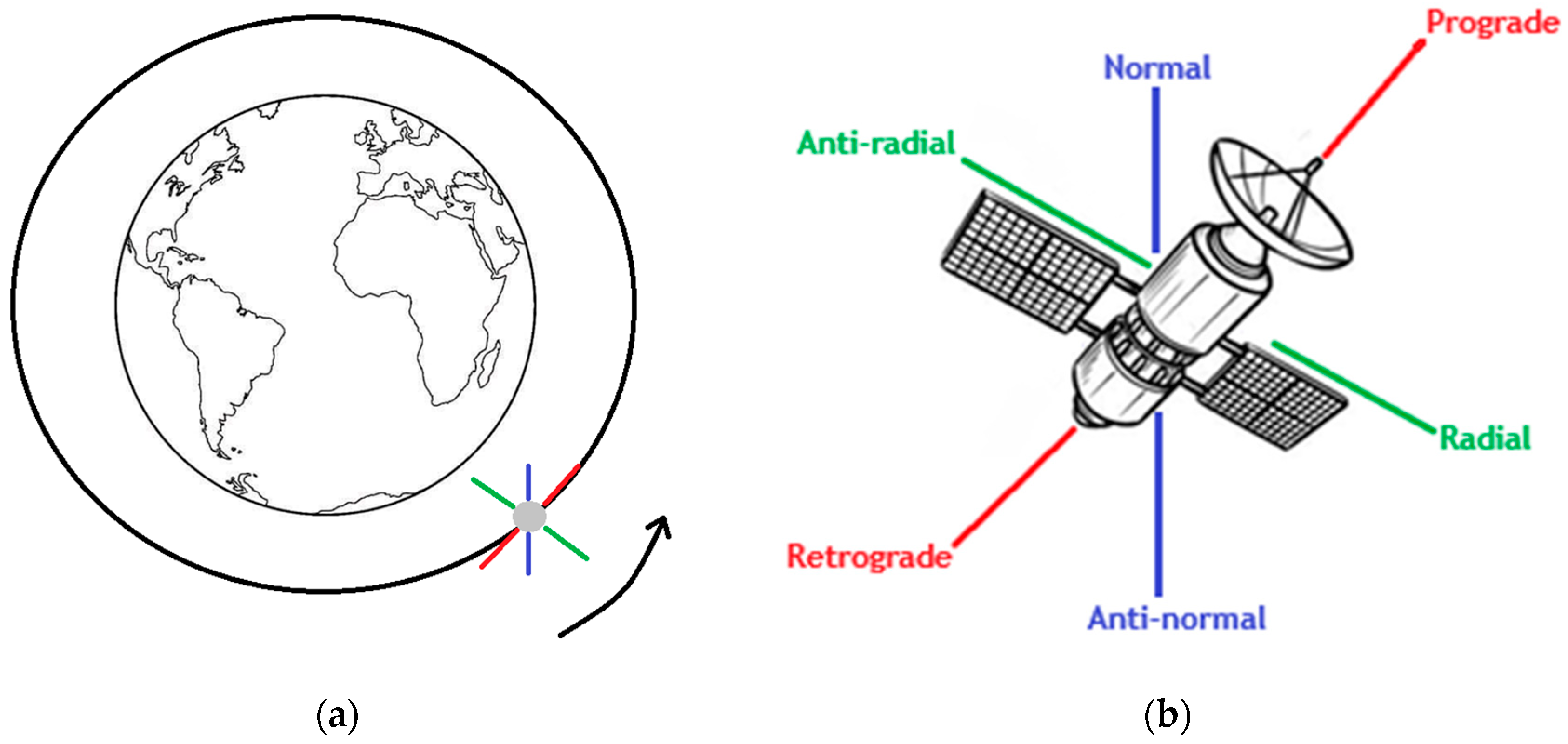
2.1. Directions of the Thrusters During Orbital Manoeuvres

Figure 1 presents a system of reference vectors for a satellite on the orbit, which is used in orbital mechanics for planning manoeuvres. The “prograde” vector (red, top-right) represents the direction of movement of the satellite and is responsible for increasing orbital speed, while the opposite “retrograde” vector (red, bottom-left) reduces the speed, lowering the orbit. The “radial” and “anti-radial” vectors (green) are perpendicular to the movement. The “radial” vector points outwards from the central body, while the “anti-radial” points towards the centre of the orbit, modifying its shape locally. Furthermore, the “normal” and “anti-normal” vectors (blue) are perpendicular to the orbit plane and are responsible for the changes in the inclination of the orbit. This system illustrates the main directions of satellite manoeuvres that influence the speed, shape, and orientation of the orbit.

2.2. Impulsive Manoeuvres

Impulsive manoeuvres are orbital transfers in which brief firings of on-board thrusters change the magnitude and direction of the satellite velocity vector instantaneously. It is assumed that during an impulsive manoeuvre, the position of the spacecraft is considered to be fixed; only the velocity changes. The key parameter in impulsive manoeuvres is the change in the velocity of the spacecraft, designated as ∆v. It is a vector, which means that both its magnitude and direction may be modified. The value of ∆v is closely linked to the weight of the consumed fuel (∆m), which is described by the following equation:

$${\displaystyle \frac{∆m}{m}}=1-e^{{\displaystyle \frac{∆v}{I_{sp}{g}_0}}},$$

(1)

$$∆v=\ln \left(1-{\displaystyle \frac{∆m}{m}}\right)I_{sp{g}_0},$$

(2)

where m is the weight of the spacecraft before burning, g₀ is standard acceleration of gravity on sea level, and I_sp is specific impulse of the propellant [7].

As suggested by Equation (1), the required weight of the propelling material during the use of an engine of a defined specific impulse I_sp shows an exponential relationship with the change in velocity. The ∆v coefficient refers to the total change in velocity that is necessary to perform the given manoeuvre. Certain manoeuvres require a series of impulses to achieve the intended goal. In such cases, the total value of ∆v is a sum of the values of the absolute changes in velocity required for each of the impulses. This means that, regardless of whether the manoeuvre involves accelerating, slowing down, or changing the direction, every one of these actions required a specific amount of fuel that must be consumed in order to perform the manoeuvre [7].

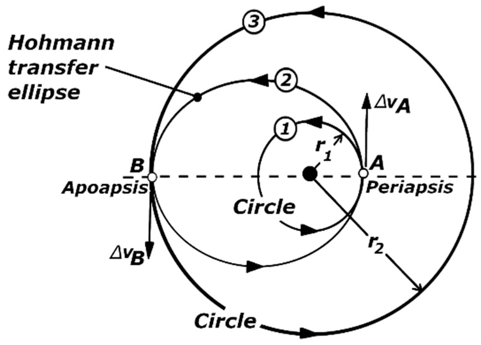
2.2.1. Hohmann Transfer

Walter Hohmann, a German engineer, is best known for his discovery of the orbital transfer manoeuvre, known as the Hohmann Transfer, which is illustrated in Figure 2. It consists of using an elliptic transfer orbit, which is tangential to two circles representing the internal and external orbit. The distance from the central body to the periapsis of the transfer ellipse matches the radius of the internal circular orbit, while the distance to the apoapsis matches the radius of the external circular orbit. During the manoeuvre, the spacecraft moves only along half of the transfer ellipse, and the movement may take place in two directions. Hohmann transfer is considered to be the most efficient in terms of fuel consumption, as it only requires two impulses—two short burns of the engine at theoretically defined points of the orbit. For example, this process may include the initial transfer of the spacecraft to the low altitude “parking orbit”, and then to a higher, circular orbit with the use of an elliptic transfer orbit, which is tangential both to the parking orbit and to the target circular orbit.

• Calculating ∆v

If the manoeuvre starts at point A, situated on the internal orbit, then a velocity increase ∆v_A in the direction of movement is required to transfer the spacecraft to the elliptical orbit with higher energy. After the satellite has moved from point A to point B, located on the external orbit, a further increase in velocity ∆v_B is required to enable the spacecraft to move to the circular orbit of even higher energy. It is worth noting that without the second increase in velocity, the spacecraft would remain on the elliptical Hohmann transfer orbit, and, as a result, it would return to the starting point A. The total fuel consumption necessary for this manoeuvre may be calculated from the equation below [7]:

$$∆v_{total}=∆v_A+∆v_B,$$

(3)

The same value of ∆v_total is required when the manoeuvre starts at point B, situated on the external circular orbit. In this case, the transfer to an internal orbit of lower energy requires a reduction in the energy of the spacecraft. To accomplish this, ∆v_A and ∆v_B must be achieved with the use of so-called retrofires. In practice, this means that the thrust of the rocket engines is directed against the direction of the spacecraft’s motion, which enables the use of the thrust force as a brake. As a result, the orbital speed of the spacecraft is reduced, which enables it to move to the lower-energy orbit [7].

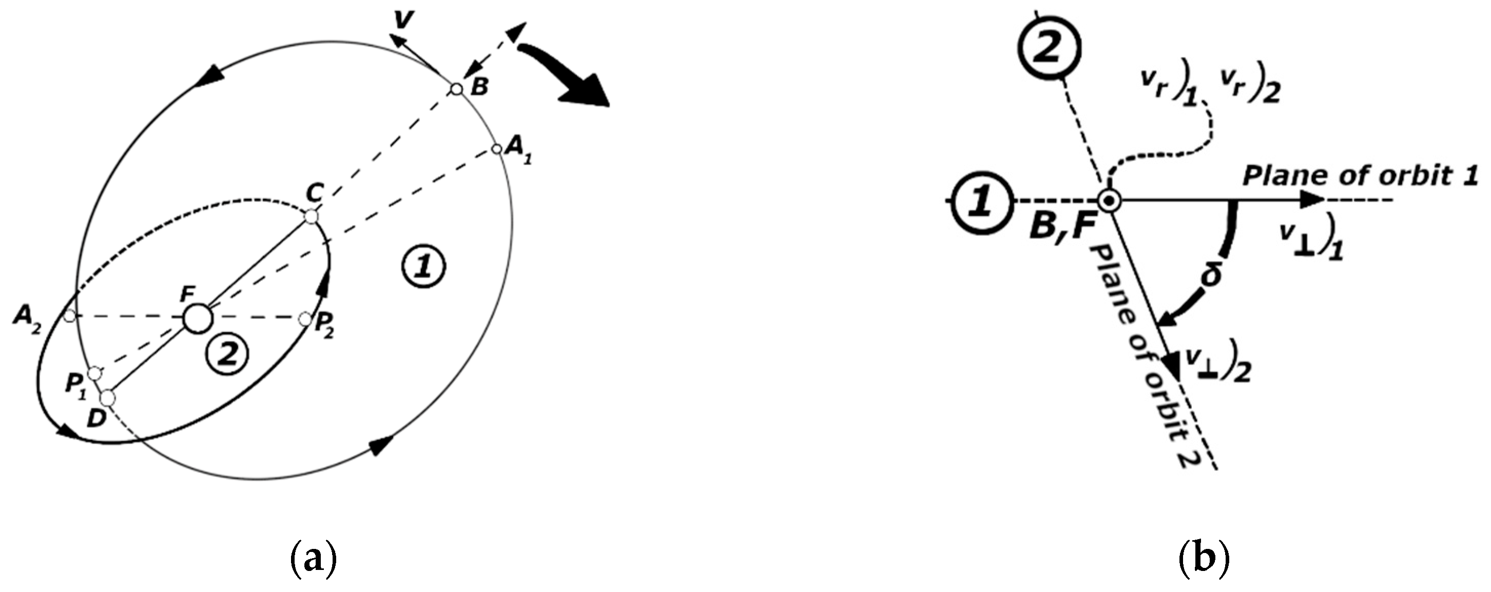
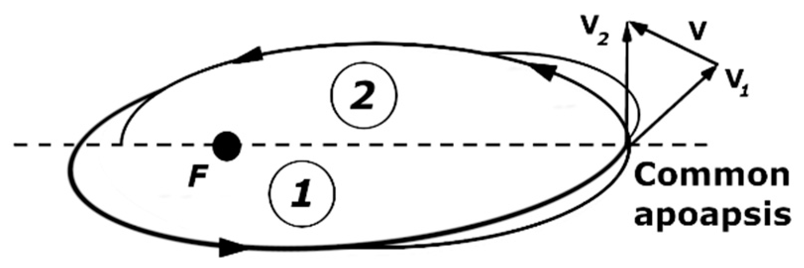
2.2.2. Manoeuvre of Changing the Orbital Plane

Changing the orbital plane is often necessary in situations when the launching point does not allow the spacecraft to reach the desired orbit directly. The latitude of the launching point has a significant influence on the inclination of the orbit: a satellite launched from the given location will automatically move on an orbit whose inclination is equal or higher than the latitude of the location. Due to that, in order to reach an orbit with an inclination other than that which results from the position of the starting point, it may become necessary to conduct a manoeuvre to change the plane of the orbit. These manoeuvres require a large ∆v, which translates into high fuel consumption [7].

Changing the orbital plane consists of modifying the direction of the perpendicular component of the velocity of the spacecraft. The angle between the initial and target perpendicular component of velocity, denoted as δ, is a dihedral angle and it is presented in Figure 3.

Similarly, as for radial velocity, the perpendicular component of velocity may also change its value during the inclination-changing manoeuvre. Orbits that have a common centre F do not have to be coplanar and are usually on different planes. Figure 3 shows two such orbits and their intersection line, marked as BD. Points A and P represent, respectively, the apoapsis and periapsis of the orbits. As the common centre F is on both orbital planes, it must also be located on their intersection line. In order for the spacecraft being on the initial orbit (orbit 1) to be able to change the plane to the target orbit (orbit 2) with a single ∆v manoeuvre, it is necessary to conduct the manoeuvre at a point where the initial orbit intersects the target orbit. Such opportunity exists only in points B and D, which are situated on the intersection line of two orbital planes [7].

• Required change in velocity

General formula to calculate ∆v for a change in the orbit plane [7]:

$$∆v=\sqrt{{\left(v_{r_2}-v_{r_1}\right)}^2+{v_{\perp 1}}^2+{v_{\perp 2}}^2-2v_{\perp 1}{v}_{\perp 2}\cos \delta }$$

(4)

To minimise ∆v for the given dihedral angle δ, two conditions have to be met:

• The radial velocity component should remain constant, i.e., $v_{r_2}-v_{r_1}=0$;
• The perpendicular velocity component should be as small as possible.

Optimum conditions occur when the initial and target orbits intersect at the apoapsis. As shown in Figure 4, if the manoeuvre is conducted in the apoapsis, the radial velocity component is $v_{r_2}=v_{r_1}=0$ for both orbits.

Additionally, in the apocentre, the azimuthal velocity components are the lowest, which allows to minimise the value of ∆v [7].

$$∆v=\sqrt{{v_1}^2+{v_2}^2-2v_1{v}_2\cos \delta },$$

(5)

If there is no change in velocity, i.e., $v_2=v_1$, the equation takes the following form:

$${∆v}_{\delta }=2v\sin {\displaystyle \frac{\delta }{2}},$$

(6)

where the lower index of δ reminds us that this is the ∆v for the exclusive rotation of the velocity vector by angle δ [7].

In conclusion, the manoeuvre of changing the orbit plane, also known as changing the inclination, is one of the most energy consuming orbital manoeuvres. Its aim is to change the inclination of the orbit, i.e., the angle of inclination of the orbital plane in relation to the reference plane, usually the plane of the planet’s equator (for satellites orbiting around the Earth) or the plane of the ecliptic (for planets and objects in the solar system). This manoeuvre is often applied when the orbit of a satellite requires modification to provide a better angle for the observation of the given area, target, or celestial body.

2.3. Methodology

This section provides a detailed description of the applied methods and approaches that have been developed based on the knowledge presented in the previous section on the current state of knowledge. The key parameters and mathematical formulas that are necessary to conduct the analyses were determined based on the literature on the problems of orbital mechanics, the properties of nanosatellites, and propulsion technologies. The presented methodology takes into consideration both the theoretical assumptions related to orbital manoeuvres and the properties of satellites, as well as the limitations that result from the characteristics of nanosatellites, such as their weight, fuel consumption, or energy capacity. Special attention was paid to the analysis of the duration of the flight of a nanosatellite over the given area with the known angle of inclination of its trajectory in reference to the equatorial plane, with a varying weight of the satellite and varying fuel weight. The authors also focused on the determination of the efficiency of various orbital manoeuvres (inclination change, Hohmann transfer) and optimising the orientation of the nanosatellite in the context of maximising the observations of a specific area. Finally, the authors attempted to choose the optimal nanosatellite in terms of fuel consumption during orbital manoeuvres.

The developed methods were based on existing formulas and models that were adapted and adjusted to the specificity of the analysed nanosatellites. The following sub-sections contain detailed descriptions of the equations used, the input parameters, and the analytical process that made it possible to conduct the simulation and to obtain the results that fulfil the predefined research objectives.

The authors used a hybrid approach, combining the analytical computational methods with computer analysis in the STK (Systems Tool Kit 12.7.1, AGI (Analytical Graphics, Inc.), Exton, PA, USA) environment. At the first stage, detailed analytical calculations were conducted, with the use of the formula and mathematical models described below. The results of the analytical calculations then served as input data for further analysis conducted in the STK 12.7.1 environment. This tool enabled the authors to perform computer simulations to verify the correctness of the preceding calculations and enable a more detailed analysis of the satellite’s trajectory, orbit parameters, and the efficiency of manoeuvres in a realistic environment that models the conditions in space. This approach ensured that the analysis was comprehensive and combined the accuracy and a theoretical basis for analytical calculations with a practical verification and visualisation in computer simulations.

• Equations used

Acceleration of gravity at the altitude of h_p:

$$g={\displaystyle \frac{G·M_Z}{{(R_Z+h_p)}^2}},$$

(7)

where G is the gravitational constant 6.6743 × 10⁻¹¹, M_Z is the weight of the Earth 5.972 × 10²⁴, R_Z is the radius of the Earth 6371, and h_p is the initial altitude. The equation is derived directly from the Newton’s law of universal gravitation. The value of g decreases with the increase in h_p, as the force of gravity decreases proportionally to the square distance from the centre of the mass of the Earth [25].

Effective exhaust velocity:

$$v_e=I_{sp}·g,$$

(8)

where I_sp is the specific impulse, and g is the acceleration of gravity. This formula describes the efficiency of a rocket engine [26].

Increase in velocity:

$$∆v=v_e·\ln {\displaystyle \frac{m_p}{m_k}},$$

(9)

where v_e is the effective exhaust velocity, m_p is the initial weight of the satellite with fuel, and m_k is the final weight of the satellite without fuel [26]. This formula results from the Tsiolkovsky equation that describes the relation between the increase in the velocity of a rocket, its effective exhaust velocity, and the ratio of the initial and final weight.

The weight of the fuel consumed to conduct the manoeuvre:

$$m_{f_{spent}}=m_p-m_k=m_p\left(1-e^{\left(-{\displaystyle \frac{∆v}{v_e}}\right)}\right),$$

(10)

m_p is the initial weight of the satellite with fuel, m_k is the final weight of the satellite without fuel, ∆v is the increase in velocity, and v_e is the effective exhaust velocity [26]. This formula was obtained by transforming the Tsiolkovsky equation and it describes the mass of fuel consumed during an orbital manoeuvre. The above formula results from the logarithmic relationship between the increase in velocity and the ratio of the weights before and after burning the fuel. The formula takes into account the fact that the amount of consumed fuel increases with the required increase in velocity and decreases for higher values of effective exhaust velocity, which reflects the improved efficiency of the propulsion system. Due to that, the formula enables a precise calculation of the demand for fuel depending on the parameters of the manoeuvre and of the propulsion system.

Duration of the impulse:

$$t={\displaystyle \frac{m_{f_{spent}}·v_e}{F}},$$

(11)

where m_fspent is the weight of consumed fuel, v_e is the effective exhaust velocity, and F is the thrust force [26]. This formula describes the duration of the impulse that is required to burn a specific amount of fuel during an orbital manoeuvre. The formula is derived from Newton’s second law of motion and the definition of the thrust force. Thrust force is related to the amount of fuel burnt in a unit of time and the effective exhaust velocity. Therefore, time may be determined as the ratio of the total weight of fuel to the rate at which it is burnt. In this way, the formula demonstrates that the duration of the impulse depends both on the efficiency of the propulsion system and on the thrust power available.

• Duration of the satellite’s flight over a given area

Inclination of the satellite’s trajectory in reference to the equator:

$$\theta =arcsin{\displaystyle \frac{\cos \mathsf{\phi }}{\sin i}},$$

(12)

where φ is the latitude, and i is the inclination of the orbit [27].

The arcsin function is used, because the θ angle is based on the trigonometric proportion $\sin \theta ={\displaystyle \frac{\cos \mathsf{\phi }}{\sin i}}$ between latitude and inclination. The application of this function enables us to determine the actual angle of inclination of the satellite’s trajectory in reference to the parallel.

Duration of the satellite’s flight over a given area:

$$T={\displaystyle \frac{L}{v_o·\cos \theta }},$$

(13)

where L is the swath width, v_o is orbital velocity, and θ is the angle of inclination of the satellite’s trajectory in reference to the equator [28]. The cosθ function adjusts the actual velocity of the satellite over Earth’s surface along the parallel.

• Determining the possible change in inclination

Possible change in inclination:

$$i_m=2·{\sin }^{-1}({\displaystyle \frac{∆v}{2v_0}}),$$

(14)

where ∆v is the increase in velocity, and v_o is the orbital velocity [7]. The formula results from the principles of orbital mechanics and geometry, which determine the change in the inclination of the orbit

During a change in inclination, an impulse is introduced that changes the direction of orbital velocity. The change in inclination is proportional to the given impulse. As inclination is defined in reference to the equatorial plane, the value of arcsin enables to calculate the angle of change in trajectory depending on the applied impulse.

Target inclination:

$$i_d=i_p-i_m,$$

(15)

where i_p is the initial inclination and i_m is the possible change in inclination. The formula results from the principle of adding or subtracting angles in the geometrical system of the orbit. The inclination change manoeuvre leads to shifting the orbital plane in reference to the equator by the i_m value, which is limited by the fuel and energy resources. The difference between the initial inclination and the possible change in inclination gives the target value, assuming that the change is subtracted from the initial inclination in the correct direction.

• Determination of the weight of fuel necessary to perform the Hohmann transfer

Initial radius of the orbit:

$$r_p=R_Z+h_p,$$

(16)

where R_Z is the radius of the Earth, and h_p is the initial altitude [7]. The formula results from the geometry of the orbit, where the initial radius of the orbit is the distance from the centre of the Earth to the satellite. Since the satellite is at the altitude h_p above the surface of the Earth, the total radius of the orbit is a sum of the radius of the Earth and this altitude.

Target radius of the orbit:

$$r_d=R_Z+h_d,$$

(17)

where R_Z is the radius of the Earth, and h_d is the target altitude [7]. The formula results from the geometry of the orbit. The radius of the target orbit is the distance from the centre of the Earth to the satellite. When the satellite reaches the target altitude, the radius of the orbit will be the sum of the radius of the Earth and this altitude.

Velocity on the initial orbit:

$$v_p=\sqrt{{\displaystyle \frac{G·M}{r_p}}},$$

(18)

where G is the gravitational constant 6.6743 × 10⁻¹¹, M_Z is the weight of the Earth 5.972 × 10²⁴, and r_p is the radius of the initial orbit [7]. The formula results from the balance of forces on the orbit. On the orbit, the satellite moves in balance between the gravity force of the Earth and the centrifugal force that results from orbital movement. The formula is derived from Newton’s second law of motion. After equalising these forces and simplifying, the formula for orbital velocity is obtained.

Velocity on the target orbit:

$$v_d=\sqrt{{\displaystyle \frac{G·M}{r_d}}},$$

(19)

where G is the gravitational constant 6.6743 × 10⁻¹¹, M_Z is the weight of the Earth 5.972 × 10²⁴, and r_d is the radius of the target orbit [7].

Velocity on the transfer orbit at the perigee:

$$v_{tp}=\sqrt{G·M({\displaystyle \frac{2}{r_p}}-{\displaystyle \frac{1}{a}})},$$

(20)

where G is the gravitational constant 6.6743 × 10⁻¹¹, M_Z is the weight of the Earth 5.972 × 10²⁴, r_p is the radius of the initial orbit, and a is the semi-major axis [7]. The formula results from the principle of energy conservation on Kepler’s orbit, where the sum of kinetic and potential energy is constant. The formula takes into account the gravitational relation between velocity and the radius of the initial orbit and the shape of the orbit (the semi-major axis).

Velocity on the transfer orbit at the apogee:

$$v_{ta}=\sqrt{G·M({\displaystyle \frac{2}{r_d}}-{\displaystyle \frac{1}{a}})},$$

(21)

where G is the gravitational constant 6.6743 × 10⁻¹¹, M_Z is the weight of the Earth 5.972 × 10²⁴, r_d is the radius of the target orbit, and a is the semi-major axis [7].

First increase in velocity:

$${∆v}_1=v_{tp}-v_p,$$

(22)

where v_tp is the velocity on the initial orbit at the perigee and v_p is the velocity on the initial orbit [7]. This formula describes the first velocity impulse required to transfer from the initial orbit to the transfer orbit. It results from the difference in the velocity that the satellite must achieve in the perigee to enter the transfer orbit.

Second increase in velocity:

$${∆v}_2=v_d-v_{ta},$$

(23)

where v_d is the velocity on the target orbit and v_ta is the velocity in the apogee on the transfer orbit [7].

Total increase in velocity:

$${∆v}_{total}={∆v}_1+{∆v}_2,$$

(24)

where ∆v₁ is the first increase in velocity and ∆v₂ is the second increase in velocity [7]. This formula defines the total increase in velocity required to perform the complete Hohmann transfer. The first impulse changes the velocity to move from the initial orbit to the transfer orbit, and the second impulse adjusts the velocity to transfer from the transfer orbit to the target orbit. The total increase in velocity is a sum of these two impulses that constitutes the total fuel cost of the manoeuvre.

Required weight of fuel:

$$m_{total}=m_p(1-e^{\left(-{\displaystyle \frac{v_e}{{∆v}_{total}}}\right)}),$$

(25)

where m_p is the initial weight of the satellite with fuel, v_e is the effective exhaust velocity, and ∆v_total is the total increase in velocity [7]. This formula is used to calculate the weight of fuel required to perform an orbital manoeuvre based on Tsiolkovsky’s rocket equation. It takes into account the effective exhaust velocity, the total increase in velocity, and the initial weight of the satellite. The formula describes the amount of fuel consumed to achieve the required change in velocity, taking into account the characteristics of the propulsion system and fuel efficiency.

• Calculating the energy required to tilt the satellite

Energy consumed by reaction wheels:

$$E=P·t,$$

(26)

where P is the power collected by reaction wheels and t is the duration of operation of these reaction wheels [28]. The formula allows for the estimation of the total energy consumption during operations related to changing the orientation of the satellite.

Loading time:

$$t_{ł}={\displaystyle \frac{E}{P_{ł}}},$$

(27)

where E is the energy consumed by reaction wheels and P_ł is the charging power of reaction wheels [28]. The formula enables to estimate how long the satellite must use its solar panels or other power sources to restore the full operational capacity.

• Presentation of the constant parameters for the analysed manoeuvres

The area that was analysed for the purposes of this research project has a surface of approx. 385 km², which corresponds to an average big city in Poland or the surface area of a typical national park. These types of areas often require various analyses, such as analysing the degree of urbanisation or the quality of trees and waters. For the purposes of this study, it was assumed that the analysed area would be the Kampinos National Park, situated near Warsaw, at the latitude of 52.2297° = 0.911 rad.

The swath width observed by the sensor mounted on the satellite depends directly on the optical parameters of the sensor and on the altitude of the orbit, and indirectly on the weight of the satellite. Increasing the weight of the satellite allows for the application of more advanced and heavier optic systems that offer a larger field of vision and higher quality of imaging. Therefore, in the first analysis (Section 3.1), the authors used a width of the swath width that increases with the weight of the satellite, to reflect the realistic structural and technological possibilities of nanosatellites. Specific values of swath width assigned to specific weights of satellites result from the assumptions concerning the configuration of the optic systems and the technical parameters of this class of devices. Specific values are presented at the further stages of the experiment to ensure consistency with the assumptions adopted for the purposes of the analysis. In the other analyses (Section 3.2, Section 3.3, Section 3.4 and Section 3.5), the authors decided to use the parameters of the MultiScape 100 CIS sensor (Simera Sense Europe BV, Technologielaan 9, 3001 Leuven, Belgium), which are listed in

Table 1. Parameters of the MultiScape 100 CIS sensor. Source: [29].

Parameter	Value	Unit
GSD at the altitude of 500 km	4.75	m
Swath width at the altitude of 500 km	19.4	km
Number of channels in the VNIR band	7	-
Spectral range	450–900	nm
Number of pixels	4096	pix
Pixel size	5.5	µm
Sensor type	“pushbroom”	-

.

The MultiScape100 CIS was designed with a specific goal in mind, i.e., to record images of the Earth with a higher level of detail and a broader range of spectral bands, while fitting inside the CubeSat format of the 3U and 6U size. The sensor is based on a CMOS matrix with a shutter and a multi-spectral filter in the visible and near-infrared spectrum (VNIR). Additionally, each channel has up to 32 digital TDI (“Time Delay Integration”) stages to improve the sensitivity and quality of the acquired images [29].

• Duration of the satellite’s flight over a given area

• Case with a variable weight of the satellite

Table 2. Presentation of the fixed parameters used in the analysis of the duration of the satellite’s flight over Kampinos National Park for a variable weight of the satellite.

Parameter	Symbol	Value	Unit
Fuel weight	mf	0.5	[kg]
Orbit altitude	h	482	[km]
Acceleration of gravity	g	8.49	$[{\displaystyle \frac{\mathrm{m}}{{\mathrm{s}}^2}}]$
Orbital velocity	vo	7.8	$[{\displaystyle \frac{\mathrm{k}\mathrm{m}}{\mathrm{s}}}]$
Thrust force	F	1	[N]
Weight of the fuel consumed to conduct the manoeuvre	mfspent	0.5	[kg]
Angle of inclination of the trajectory in reference to the equator at the orbit inclination of 97°	θ	0.655	[rad]

shows the key parameters related to the orbital motion of the satellite and its observation capacity. It includes the weight of fuel, thrust force, and the altitude of the orbit, as well as orbital velocity and acceleration of gravity that influence the satellite.

• Case with variable fuel weight

Table 3. Presentation of the fixed parameters used in the analysis of the duration of the satellite’s flight over Kampinos National Park for a variable fuel weight.

Parameter	Symbol	Value	Unit
Initial weight of the satellite	mp	15	[kg]
Orbit altitude	h	482	[km]
Acceleration of gravity	g	8.49	$[{\displaystyle \frac{\mathrm{m}}{{\mathrm{s}}^2}}]$
Orbital velocity	vo	7.8	$[{\displaystyle \frac{\mathrm{k}\mathrm{m}}{\mathrm{s}}}]$
Thrust force	F	1	[N]
Swath width	L	19.4	[km]
Angle of inclination of the trajectory in reference to the equator at the orbit inclination of 97°	θ	0.655	[rad]

presents the initial weight of the satellite, orbit altitude, orbital velocity, and the active acceleration of gravity that influence the dynamics of the flight.

• Determining the possible change in inclination

Table 4. Presentation of the fixed parameters used in the analysis of the possible change in inclination.

Parameter	Symbol	Value	Unit
Initial inclination of the orbit	ip	97	[°]
Orbit altitude	h	482	[km]
Acceleration of gravity	g	8.49	$[{\displaystyle \frac{\mathrm{m}}{{\mathrm{s}}^2}}]$
Orbital velocity	vo	7.8	$[{\displaystyle \frac{\mathrm{k}\mathrm{m}}{\mathrm{s}}}$]
Thrust force	F	1	[N]

presents the initial inclination of the orbit, orbit altitude, and the acceleration of gravity that affects the satellite, influencing its movement. The orbital velocity and thrust force determine the dynamic conditions that are necessary to conduct the inclination change manoeuvre.

• Determination of the weight of fuel necessary to perform the Hohmann transfer

Table 5. Presentation of the fixed parameters used in the analysis of the amount of fuel necessary to perform the Hohmann transfer.

Parameter	Symbol	Value	Unit
Initial orbit altitude	hp	482	[km]
Target orbit altitude	hd	550	[km]
Radius of the Earth	RZ	6371	[km]
Acceleration of gravity	g	8.49	[${\displaystyle \frac{\mathrm{m}}{{\mathrm{s}}^2}}$]
Gravitational constant	G	6.674 × 10−11	[${\displaystyle \frac{{\mathrm{m}}^3}{{\mathrm{k}\mathrm{g}·\mathrm{s}}^2}}$]
Weight of the Earth	MZ	5.972 × 1024	[kg]
Initial radius of the orbit	rp	6853	[km]
Target radius of the orbit	rd	6921	[km]
Velocity on the initial orbit	vp	7626.45	[${\displaystyle \frac{\mathrm{m}}{\mathrm{s}}}$]
Velocity on the target orbit	vd	7588.89	[${\displaystyle \frac{\mathrm{m}}{\mathrm{s}}}$]
Semi-major axis	a	6887	[km]
Velocity on the transfer orbit in perigee	vtp	7645.25	[${\displaystyle \frac{\mathrm{m}}{\mathrm{s}}}$]
Velocity on the transfer orbit in apogee	vta	7570.14	[${\displaystyle \frac{\mathrm{m}}{\mathrm{s}}}$]
First increase in velocity	∆v1	18.80	[${\displaystyle \frac{\mathrm{m}}{\mathrm{s}}}$]
Second increase in velocity	∆v2	18.76	[${\displaystyle \frac{\mathrm{m}}{\mathrm{s}}}$]
Total increase in velocity	Δvtotal	37.56	[${\displaystyle \frac{\mathrm{m}}{\mathrm{s}}}$]
Orbital velocity	vo	7.8	[${\displaystyle \frac{\mathrm{k}\mathrm{m}}{\mathrm{s}}}$]
Thrust force	F	1	[N]

presents the parameters of the initial and target orbits, including orbital altitudes, corresponding orbital radii, and orbital velocities for both positions. Additionally, the velocities at the perigee and apogee of the transfer orbit are provided. Two velocity increments (Δv₁ i Δv₂) were also calculated, which together constitute the total velocity increment (Δv_total) required to perform the manoeuvre. The target orbit parameters reflect a typical Sun-synchronous orbit used in Earth observation missions, chosen to optimize coverage of the area of interest at specific times during the nanosatellite’s passes. These parameters were determined based on mission requirements, particularly the frequency of passes over the area of interest (AOI), effective ground coverage, and ensuring adequate observation time. The first orbital manoeuvre (Δv₁) was executed approximately two hours after the nanosatellite was placed in the initial orbit, initiating the Hohmann transfer manoeuvre. The main acceleration (Δv₂) completing the transfer and shaping the target orbit was performed at the apogee of the transfer orbit, which occurred during the nanosatellite’s second revolution.

• Calculating the energy required to tilt the satellite

Table 6. Presentation of the fixed parameters used in the analysis of the of the energy required to tilt the satellite.

Parameter	Symbol	Value	Unit
Weight of the satellite without fuel	ms	4.5	[kg]
Fuel weight	mf	0.5	[kg]
Weight of the satellite with fuel	msf	5	[kg]
Satellite size along the x axis	-	0.1	[m]
Satellite size along the y axis	-	0.2	[m]
Satellite size along the x axis	-	0.3	[m]
Moment of inertia	Iz	0.021	[kg·m2]
Slew rate	-	5	[°]
Power consumption in the stable state (1000 RPM)	P	0.45	[W]
Charging power of the solar panels	Pł	70	[W]

presents the fixed parameters necessary for the analysis of the energy required to tilt the satellite. They include the satellite’s weight without fuel, fuel weight, and the total weight of the satellite with fuel that influence the moment of inertia and motion dynamics. The parameters also include the slew rate that defines the rate of changing the orientation of the satellite. Power consumption in the stable state and the available charging power of solar panels determine the energy balance of the system that is necessary to perform the manoeuvre.

3. Results

The analysis presented below was conducted as there were no existing studies on the optimisation of nanosatellites in terms of the maximisation of the duration of flight over specific areas of interest. The research results point to the fact that an appropriate selection of the orbit parameters and of the weight of the satellite and fuel significantly influence the efficiency of the operational mission.

3.1. Analysis for a Variable Weight of the Satellite

The analysis was conducted for several different assumptions. The first one states that the fuel weight is constant, and it is 0.5 kg. The weight of the satellite, however, takes different values. Depending on the quality of the telescope, in may range from 8 to 18 kg (satellite classes: nano and nano+).

Table 7. Presentation of the analysis results on the impact of sensor parameters (related to the satellite’s mass) on the overflight time above Kampinos National Park.

Initial Weight of the Satellite mp [kg]	End Weight of the Satellite mk [kg]	Specific Impulse Isp [s]	Effective Exhaust Velocity ${\mathbf{v}}_{\mathbf{e}}\left[\frac{\mathbf{m}}{\mathbf{s}}\right]$	Increase in Velocity $∆\mathbf{v}\left[\frac{\mathbf{m}}{\mathbf{s}}\right]$	Impulse Duration t [s]	Swath Width L [km]	Duration of the Satellite’s Flight over the Area of Interest T [s]
8	7.5	180	1528.20	98.63	764.10	15.0	2.44
9	8.5	190	1613.10	92.20	806.55	16.0	2.61
10	9.5	200	1698.00	87.10	849.00	17.0	2.77
11	10.5	210	1782.90	82.94	891.45	17.5	2.85
12	11.5	215	1825.35	77.69	912.67	18.0	2.93
13	12.5	220	1867.80	73.26	933.90	18.5	3.01
14	13.5	225	1910.25	69.47	955.13	19.0	3.10
15	14.5	230	1952.70	66.20	976.35	19.4	3.16
16	15.5	235	1995.15	63.34	997.58	19.8	3.23
17	16.5	240	2037.60	60.83	1018.80	20.2	3.29
18	17.5	250	2122.50	59.79	1061.25	21.0	3.42

presents the results of the analysis regarding the influence of sensor-related satellite parameters, particularly those associated with satellite mass, on the overflight time above Kampinos National Park. The parameters include the initial and final mass of the satellite, specific impulse, and effective exhaust velocity, which together determine the ∆v and the impulse duration required for the manoeuvre.

The objective of the conducted analysis was to examine the impact of satellite mass, indirectly reflected by the swath width of the onboard sensor, on the overpass time above Kampinos National Park. The results indicate that as the satellite mass increases, the overpass time over the analysed area also extends. This effect does not result directly from the satellite’s mass but from the assumption that heavier satellites are capable of carrying more advanced sensors with wider swath widths. Such sensors enable longer imaging times for a given area, which translates into an extended observation time.

The results of analyses performed using STK 12.7.1 (Systems Tool Kit) software for a low circular Earth orbit (altitude: 482 km, inclination: 97°) are close to the values calculated analytically, confirming the correctness of the adopted assumptions and equations describing the satellite’s overpass time over the area of interest. This is illustrated in Figure 5, which presents a visualisation of the satellite's observation swath during a single pass over Kampinos National Park. For instance, for a satellite with a mass of 13 kg and a sensor swath width of 18.5 km, the analytically calculated overpass time was 3.01 s, while the STK 12.7.1simulation indicated 2.65 s (total coverage: 13.26 s). Additional results obtained in STK 12.7.1 include a satellite with a mass of 8 kg and a swath width of 15 km, for which the overpass time was approximately 2.15 s (analytically: 2.44 s), and a satellite with a mass of 18 kg and a swath width of 21 km, for which this time was approximately 3.01 s (analytically: 3.42 s). For all analysed configurations, the differences between analytical calculations and simulation results fell within an acceptable error margin of 10–15%. Slight differences between the results may be caused by the advanced modelling in STK 12.7.1, which takes into account additional orbital perturbations, such as the influence of the flattening of the Earth (the J2 model), drag on Low Earth Orbits (LEOs) and the dynamic adjustment of the satellite’s trajectory in real time. For the purposes of analytical calculations, a simplified geometry of the orbit and an ideal field of gravity were assumed, which eliminates the effects discussed above. Moreover, the differences may result from the numerical precision of the simulation, temporal resolution of calculations, and potential rounding up of certain input values, such as swath width or orbital velocity. It is also worth noting that the STK 12.7.1 software operates on a dynamic trajectory of the satellite, while analytical calculations treat the time and satellite positions as points. In conclusion, the comparison of results shows that the values obtained in the numerical and analytical analyses are compatible, with slight differences that result from the fact that STK 12.7.1 takes into account more detailed physical parameters. Detailed analyses and the conclusions that result from the calculations performed are presented and discussed in Section 4—Discussion.

3.2. Analysis for a Variable Weight of Fuel

On the other hand, the second analysis is based on the assumption that the initial weight of the satellite is 15 kg, and the fuel weight ranges from 0.3 to 0.7 kg, at intervals of 0.05 kg.

Table 8. Presentation of the results of the analysis of the duration of the satellite’s flight over Kampinos National Park for a variable weight of fuel.

End Weight of the Satellite mk [kg]	Fuel Weight mf [kg]	Specific Impulse Isp [s]	Effective Exhaust Velocity ${\mathbf{v}}_{\mathbf{e}}\left[\frac{\mathbf{m}}{\mathbf{s}}\right]$	Increase in Velocity $∆\mathbf{v}\left[\frac{\mathbf{m}}{\mathbf{s}}\right]$	Weight of Fuel Spent to Perform the Manoeuvre mfspent [kg]	Duration of the Impulse t [s]	Duration of the Satellite’s Flight over the Area of Interest T [s]
14.70	0.30	200	1698.00	34.30	0.30	509.40	3.16
14.65	0.35	210	1782.90	42.09	0.35	624.01	3.16
14.60	0.40	215	1825.35	49.34	0.40	730.14	3.16
14.55	0.45	218	1850.82	56.37	0.45	832.87	3.16
14.50	0.50	220	1867.80	63.32	0.50	933.90	3.16
14.45	0.55	225	1910.25	71.36	0.55	1050.64	3.16
14.40	0.60	230	1952.70	79.71	0.60	1171.62	3.16
14.35	0.65	235	1995.15	88.39	0.65	1296.85	3.16
14.30	0.70	240	2037.60	97.38	0.70	1426.32	3.16

presents the results of the analysis of the influence of variable fuel weight on the parameters of the orbital manoeuvre of a satellite of the initial weight of 15 kg. As the weight of fuel increases from 0.3 kg to 0.7 kg, an increase in the specific impulse and effective exhaust velocity is noted, which leads to a growing increase in velocity and duration of the impulse. The duration of the satellite’s flight over Kampinos National Park remains constant and is 3.16 s, which suggests that the analysed parameters do not affect the geometry of the observation trajectory. More detailed analyses and the conclusions that result from the calculations performed are presented and discussed in Section 4—Discussion.

3.3. Analysis of the Possible Change in Inclination

Further analyses concerned performing orbital manoeuvres by nanosatellites in order to maximise the duration of the satellite’s flight over the area of interest. The aim of the third analysis was to find an orbit with the inclination that will be optimised in terms of fuel consumption while performing the manoeuvre of changing the inclination of the orbit and the duration of flight over the given area. The analysis took into consideration two cases: (1) The weight of fuel is constant and is 0.5 kg, but the weight of the satellite, however, takes different values. Depending on the quality of the telescope, it may range from 8 to 18 kg. (2) The initial weight of the satellite is 15 kg, and the fuel weight ranges from 0.3 to 0.7 kg, at intervals of 0.05 kg.

Table 9. Presentation of the results of the analysis of the possible change in inclination.

Initial Weight of the Satellite mp [kg]	End Weight of the Satellite mk [kg]	Weight of Fuel mf [kg]	Specific Impulse Isp [s]	Effective Exhaust Velocity ${\mathbf{v}}_{\mathbf{e}}\left[\frac{\mathbf{m}}{\mathbf{s}}\right]$	Increase in Velocity $∆\mathbf{v}\left[\frac{\mathbf{m}}{\mathbf{s}}\right]$	Possible Change in Inclination im [rad]	Possible Change in Inclination im2 [°]	Target Inclination id [rad]	Target Inclination id2 [°]	Inclination of the Trajectory in Reference to the Equator After the Manoeuvre θm [rad]	Swath Width L [km]	Duration of the Satellite’s Flight over the Area of Interest T [s]
8	7.50	0.50	180	1528.20	98.63	0.013	0.72	1.680	96.28	0.752	15.0	2.63
9	8.50	0.50	190	1613.10	92.20	0.012	0.68	1.681	96.32	0.775	16.0	2.87
10	9.50	0.50	200	1698.00	87.10	0.011	0.64	1.682	96.36	0.797	17.0	3.12
11	10.50	0.50	210	1782.90	82.94	0.011	0.61	1.682	96.39	0.817	17.5	3.28
12	11.50	0.50	215	1825.35	77.69	0.010	0.57	1.683	96.43	0.845	18.0	3.48
13	12.50	0.50	220	1867.80	73.26	0.009	0.54	1.684	96.46	0.873	18.5	3.69
14	13.50	0.50	225	1910.25	69.47	0.009	0.51	1.684	96.49	0.899	19.0	3.91
15	14.50	0.50	230	1952.70	66.20	0.008	0.49	1.684	96.51	0.924	19.4	4.13
16	15.50	0.50	235	1995.15	63.34	0.008	0.47	1.685	96.53	0.949	19.8	4.36
17	16.50	0.50	240	2037.60	60.83	0.008	0.45	1.685	96.55	0.972	20.2	4.59
18	17.50	0.50	250	2122.50	59.79	0.008	0.44	1.685	96.56	0.982	21.0	4.85
15	14.65	0.35	210	1782.90	42.09	0.005	0.31	1.688	96.69	1.263	19.4	8.22
15	14.60	0.40	215	1825.35	49.34	0.006	0.36	1.687	96.64	1.114	19.4	5.64
15	14.55	0.45	218	1850.82	56.37	0.007	0.41	1.686	96.59	1.019	19.4	4.74
15	14.50	0.50	220	1867.80	63.32	0.008	0.47	1.685	96.53	0.949	19.4	4.27
15	14.45	0.55	225	1910.25	71.36	0.009	0.52	1.684	96.48	0.886	19.4	3.93
15	14.40	0.60	230	1952.70	79.71	0.010	0.59	1.683	96.41	0.834	19.4	3.70
15	14.35	0.65	235	1995.15	88.39	0.011	0.65	1.682	96.35	0.791	19.4	3.54
15	14.30	0.70	240	2037.60	97.38	0.012	0.72	1.680	96.28	0.756	19.4	3.42

presents the results of the analysis of the influence of the initial weight of the satellite and variable fuel weight on the possible change in the inclination of the orbit. With the increase in the effective exhaust velocity and growing increase in velocity, a gradual increase in the possible change in inclination is observed. Detailed results reveal that higher fuel weight and specific impulse enable a larger change in inclination, while at the same time prolonging the duration of the manoeuvre.

As illustrated in Figure 6, the simulation of the inclination change manoeuvre demonstrates the orbital geometry before and after the adjustment. The comparison of the results of analytical calculations and computer simulation in the STK 12.7.1 software for the inclination change manoeuvre for a nanosatellite of the weight of 8 kg, a difference in the increase in velocity was noted, of 98.63 ${\displaystyle \frac{\mathrm{m}}{\mathrm{s}}}$ in the analytical calculations and 95.84 ${\displaystyle \frac{\mathrm{m}}{\mathrm{s}}}$ in STK 12.7.1, which means a difference of approx. 2.79 ${\displaystyle \frac{\mathrm{m}}{\mathrm{s}}}$.

This difference is caused mainly by the higher accuracy of the STK 12.7.1 numerical model, which takes into account additional factors, such as propulsion characteristics and potential environmental influences that are not taken into account by simplified analytical assumptions. In spite of that, both approaches are consistent, and the results of STK 12.7.1 simulations are more realistic in the context of the actual conditions. More detailed conclusions are provided in Section 4—Discussion.

3.4. Analysis of the Weight of Fuel Necessary to Perform the Hohmann Transfer

The aim of the fourth analysis was to check the weight of fuel that is necessary to perform the Hohmann transfer. The analysis took into consideration two cases: (1) the weight of fuel is constant and is 0.5 kg, but the weight of the satellite, however, takes different values. Depending on the quality of the telescope, in may range from 8 to 18 kg. (2) the initial weight of the satellite is 15 kg, and the fuel weight ranges from 0.3 to 0.7 kg, at intervals of 0.05 kg.

Table 10. Presentation of the results of the analysis of the weight of fuel necessary to perform the Hohmann transfer.

Initial Weight of the Satellite mp [kg]	Specific Impulse Isp [s]	Effective Exhaust Velocity ${\mathbf{v}}_{\mathbf{e}}\left[\frac{\mathbf{m}}{\mathbf{s}}\right]$	Fuel Weight Required mtotal [kg]
8	180	1527.69	0.194
9	190	1612.57	0.207
10	200	1697.44	0.219
11	210	1782.31	0.229
12	215	1824.75	0.244
13	220	1867.18	0.259
14	225	1909.62	0.273
15	230	1952.05	0.286
16	235	1994.49	0.298
17	240	2036.93	0.311
18	250	2121.80	0.316
15	200	1697.44	0.328
15	210	1782.31	0.313
15	215	1824.75	0.306
15	218	1850.21	0.301
15	220	1867.18	0.299
15	225	1909.62	0.292
15	230	1952.05	0.286
15	235	1994.49	0.280
15	240	2036.93	0.274

presents the results of the analysis of the fuel weight required to perform the Hohmann transfer depending on the initial weight of the satellite and the specific impulse. As the specific impulse and effective exhaust velocity increase, a gradual decrease in the required weight of fuel is observed, which means that the engine is more efficient at higher values.

Figure 7 presents the Hohmann transfer, performed to raise the orbital altitude from 482 km to 550 km, resulting in a total increase of 68 km. The comparison of the results of analytical calculations and STK 12.7.1 simulations revealed that the values were very similar, where in the simulation for a satellite weighing 8 kg, the fuel consumption was 0.180 kg, while the result of analytical calculations was 0.194 kg. The difference between these results is only 0.014 kg. This slight difference may result from several factors. First and foremost, the simulation in the STK 12.7.1 environment accounts for more advanced gravitational models and perturbation effects significant for low Earth orbit, such as the Earth’s ellipsoidal shape (J2), irregularities in the gravitational field, atmospheric drag, and potential third-body interactions from the Sun or Moon. On the other hand, analytical calculations are typically based on simplified assumptions, such as the spherical symmetry of the Earth and constant gravitational acceleration, and do not consider such perturbations. Additionally, differences may arise from numerical rounding in the STK 12.7.1 environment, which takes into account variable conditions during an actual manoeuvre, whereas analytical methods assume an impulsive manoeuvre executed instantaneously and precisely at a predetermined orbital point. The comparison of both approaches thus serves as an indirect assessment of the impact of orbital perturbations while maintaining the clarity and utility of the analytical model for preliminary mission planning. Detailed conclusions are presented in Section 4—Discussion.

3.5. Analysis of the Energy Required to Tilt the Satellite by a Specific Angle

The previously conducted analyses lead to the conclusion that the manoeuvres that may be performed in order to maximise the duration of flight of the satellite over a given area are those whose final effects do not bring satisfactory results due to the small amount of fuel available in the satellite. Due to that, the authors decided to conduct an analysis to consider tilting the nanosatellite together with the telescope to prolong the time spent by the satellite over the area of interest. The analysis presented below was conducted for the values of parameters of the M6P satellite by NanoAvionics (Kongsberg NanoAvionics UAB, Mokslininkų g. 2A, LT-08412 Vilnius, Lithuania) [30].

Table 11. Presentation of the results of the analysis of the energy required to tilt the satellite by a specific angle.

Tilt Angle Δθ [°]	Duration of the Manoeuvre t [s]	Energy Consumed by Reaction Wheels E [J]	Charging Time tł [s]
1	0.20	0.09	0.00129
2	0.40	0.18	0.00257
3	0.60	0.27	0.00386
4	0.80	0.36	0.00514
5	1.00	0.45	0.00643
6	1.20	0.54	0.00771
7	1.40	0.63	0.00900
8	1.60	0.72	0.01029
9	1.80	0.81	0.01157
10	2.00	0.90	0.01286
11	2.20	0.99	0.01414
12	2.40	1.08	0.01543
13	2.60	1.17	0.01671
14	2.80	1.26	0.01800
15	3.00	1.35	0.01929
16	3.20	1.44	0.02057
17	3.40	1.53	0.02186
18	3.60	1.62	0.02314
19	3.80	1.71	0.02443
20	4.00	1.80	0.02571
21	4.20	1.89	0.02700
22	4.40	1.98	0.02829
23	4.60	2.07	0.02957
24	4.80	2.16	0.03086
25	5.00	2.25	0.03214
26	5.20	2.34	0.03343
27	5.40	2.43	0.03471
28	5.60	2.52	0.03600
29	5.80	2.61	0.03729
30	6.00	2.70	0.03857

presents the results of the analysis of the energy consumption by reaction wheels while tilting the satellite by a specific angle. As the tilt angle increases, a linear increase in the duration of the manoeuvre and of the fuel consumed is observed, which, in turn, leads to the proportional extension of the charging time of the power supply system.

Figure 8 shows the tilt of the sensor with the satellite platform and the coverage of the Kampinos National Park. The sensor installed on a satellite has a specific tilt angle that allows for precise observations of the defined geographic region. This is presented in the illustration as the range of the vision field of the sensor. Detailed conclusions and the interpretation of results are provided in Section 4—Discussion.

3.6. Selection of the Optimum Nanosatellite Dedicated to Maximise the Specific Operational Task

Based on the previous analyses, the authors decided to select the optimum nanosatellite dedicated to capture images of a specific area of interest. The sample calculations provided below are based on the values of specific parameters of the M6P satellite from NanoAvionics [30].

The analysis of the manoeuvre of transfer onto a higher orbit was conducted with great precision and an accuracy of up to 1 m, which will enable a precise determination of the influence of changes in the orbital parameters on the efficiency of the mission.

The force of atmospheric drag acts on the satellite that is moving on a low Earth orbit (LEO) in the rarefied atmosphere. The formula to calculate drag is derived from basic fluid dynamics:

$$F_D={\displaystyle \frac{1}{2}}·\rho ·v^2·C_D·A=0.00000135\mathrm{N},$$

(28)

where ρ is the density of the atmosphere at the altitude h. This parameter describes the number of molecules that interact with the satellite in a unit of volume. Atmospheric density decreases exponentially with increasing altitude. At the altitude h = 500 km, in the thermosphere, air density is extremely low. The atmospheric density at 500 km is 10⁻¹² ${\displaystyle \frac{\mathrm{k}\mathrm{g}}{{\mathrm{m}}^3}}.$ This value is comparable to that of the density in the vacuum in outer space. v is the orbital speed. On a low Earth orbit, the orbital speed is approx. v = 7.8 ${\displaystyle \frac{\mathrm{k}\mathrm{m}}{\mathrm{s}}}.$ The force of drag increases with the square of velocity, as higher velocity means stronger collisions with atmospheric particles. C_D is aerodynamic drag coefficient. This is a dimensionless coefficient that determines how an object reacts to a flow of gas (e.g., atmosphere). For typical satellites on low Earth orbits, this coefficient is C_D = 2.2. The value C_D = 2.2 was obtained from research on the aerodynamic drag of CubeSats on low Earth orbits. A is the frontal surface of the satellite. This surface interacts with the flow of the atmosphere. It is assumed that the frontal surface of the satellite is A = 0.02 ${\mathrm{m}}^2$, as the analysed satellite has the dimensions of 0.1 × 0.2 × 0.3 m, and the smallest possible frontal surface is assumed by default, so as to minimise the drag.

Then, the loss of orbital energy was calculated, from the formula to calculate energy loss that results from the work of the drag force.

$$∆E=F_D·v·∆t=27307 \mathrm{J},$$

(29)

where F_D = 0.00000134 N, v is orbital velocity. On a low Earth orbit, the orbital speed is approx. v = 7.8 ${\displaystyle \frac{\mathrm{k}\mathrm{m}}{\mathrm{s}}}.$ The force of drag increases with the square of velocity, as higher velocity means stronger collisions with atmospheric particles. ∆t is time [s] for a month.

The next step consisted of calculating the decrease in altitude ∆h. The drop in the altitude of the orbit results from the loss of orbital energy caused by drag. It was calculated based on the relation between energy and orbit altitude:

$$∆h=-{\displaystyle \frac{∆E}{m·g\left(h\right)}}=-643\mathrm{m},$$

(30)

where ∆E = 27307 J, m is the weight of the satellite. This value is necessary to calculate the proportion of energy loss per unit of weight. In the analysed case, the satellite has a weight of m = 5 kg. g(h) is the acceleration of gravity. The altitude of the orbit influences the value of g(h), which decreases with altitude as the force of gravity diminishes on higher orbits. g(h) = 8.49 ${\displaystyle \frac{\mathrm{m}}{{\mathrm{s}}^2}}$.

Then, the total decrease in altitude during half a year ∆h_total was calculated:

$${∆h}_{total}=∆h·6=-3860\mathrm{m},$$

(31)

This means that the satellite’s orbit will drop by 3860 m over a period of six months.

Then, the required number of manoeuvres was determined. The authors considered the efficiency of orbital manoeuvres, where increasing the orbit by 643 m will be a reasonable compromise between the number of manoeuvres and the amount of fuel necessary. The lower the increase in altitude per a single manoeuvre, the more manoeuvres have to be performed, which increases the complexity of the mission. However, increasing the orbit by higher values (e.g., by 2 km at once) would require more fuel per a single manoeuvre, which might exceed the capacity of the satellite. In the analyses for low Earth orbits, changing the altitude by approx. 1 km causes a relatively small change in velocity (∆v), which facilitates fuel management and orbit control, as the manoeuvres are easier to plan and perform. The strategy that involves more frequent manoeuvres prevents the degradation of the orbit, as the drops are corrected more often. Therefore, ∆h_manewr ≈ 643 m.

$$numberofmanouevres={\displaystyle \frac{\left|{∆h}_{total}\right|}{{∆h}_{manouevre}}}={\displaystyle \frac{\left|-3860\right|}{643}}=6,$$

(32)

Then, the increase in velocity (∆v) was calculated for one manoeuvre:

$${∆v}_1=\sqrt{{\displaystyle \frac{G{M}_Z}{r_{start}}}}\left(\sqrt{{\displaystyle \frac{2r_{target}}{r_{start}+r_{target}}}}-1\right)=5.66{\displaystyle \frac{\mathrm{m}}{\mathrm{s}}},$$

(33)

$${∆v}_2=\sqrt{{\displaystyle \frac{G{M}_Z}{r_{target}}}}\left(\sqrt{{\displaystyle \frac{2r_{start}}{r_{start}+r_{target}}}}-1\right)=5.66{\displaystyle \frac{\mathrm{m}}{\mathrm{s}}},$$

(34)

$${∆v}_{total}=\left|{∆v}_1\right|+\left|{∆v}_2\right|=11{\displaystyle \frac{\mathrm{m}}{\mathrm{s}}},$$

(35)

where G is the gravitational constant 6.6743 × 10⁻¹¹, M_Z is the weight of the Earth 5.972 × 10²⁴, h_start is the initial altitude before each manoeuvre (482 − 0.643 = 481.357 km), r_start is the radius of the initial orbit 6852.357, and r_target is the radius of the target orbit 6853.

The next stage involved calculating the amount of fuel necessary to perform the manoeuvre:

$$∆m=m·\left(1-e^{{\displaystyle \frac{-∆v}{g·I_{sp}}}}\right)=0.026\mathrm{k}\mathrm{g},$$

(36)

where ∆v = 11 ${\displaystyle \frac{\mathrm{m}}{\mathrm{s}}}$, m = 5 kg, g = 8.49 ${\displaystyle \frac{\mathrm{m}}{{\mathrm{s}}^2}}$, I_sp = 220 s.

The final stage consisted of calculating the total weight of fuel required to perform six manoeuvres over a period of six months:

$${∆m}_{total}=∆m·6=0.157\mathrm{k}\mathrm{g},$$

(37)

where ∆m = 0.026 kg.

Table 12. Presentation of the results of the analysis concerning the selection of the optimum nanosatellite.

Initial Weight of the Satellite mp [kg]	Fuel Weight mf [kg]	Specific Impulse Isp [s]	Frontal Surface of the Satellite A [m2]	Drag Force FD [N]	Loss of Orbital Energy ΔE [J]	Drop in Altitude in One Month ∆h [m]	Total Drop in Altitude in Six Months ∆htotal [m]	Required Weight of Fuel Δm [kg]	Total Required Weight of Fuel Δmtotal [kg]
8	0.50	180	0.02	0.00000135	27,306.86	−402	−2412	0.050	0.301
9	0.50	190	0.02	0.00000135	27,306.86	−357	−2144	0.053	0.321
10	0.50	200	0.02	0.00000135	27,306.86	−322	−1930	0.056	0.338
11	0.50	210	0.03	0.00000203	40,960.29	−439	−2632	0.059	0.355
12	0.50	215	0.03	0.00000203	40,960.29	−402	−2412	0.063	0.378
13	0.50	220	0.03	0.00000203	40,960.29	−371	−2227	0.067	0.400
14	0.50	225	0.03	0.00000203	40,960.29	−345	−2068	0.070	0.421
15	0.50	230	0.03	0.00000203	40,960.29	−322	−1930	0.074	0.442
16	0.50	235	0.04	0.00000270	54,613.72	−402	−2412	0.077	0.461
17	0.50	240	0.04	0.00000270	54,613.72	−378	−2270	0.080	0.480
18	0.50	250	0.04	0.00000270	54,613.72	−357	−2144	0.081	0.488
15	0.30	200	0.03	0.00000203	40,960.29	−322	−1930	0.085	0.508
15	0.35	210	0.03	0.00000203	40,960.29	−322	−1930	0.081	0.483
15	0.40	215	0.03	0.00000203	40,960.29	−322	−1930	0.079	0.472
15	0.45	218	0.03	0.00000203	40,960.29	−322	−1930	0.078	0.466
15	0.50	220	0.03	0.00000203	40,960.29	−322	−1930	0.077	0.462
15	0.55	225	0.03	0.00000203	40,960.29	−322	−1930	0.075	0.451
15	0.60	230	0.03	0.00000203	40,960.29	−322	−1930	0.074	0.442
15	0.65	235	0.03	0.00000203	40,960.29	−322	−1930	0.072	0.432
15	0.70	240	0.03	0.00000203	40,960.29	−322	−1930	0.071	0.423
5	0.50	220	0.02	0.00000135	27,306.86	−643	−3860	0.026	0.154

presents the results of the analysis aimed at selecting the optimum nanosatellite configuration based on parameters such as initial and fuel weight, specific impulse, drag force, orbital energy loss, and altitude drop over time.

4. Discussion

4.1. Discussion of the Results of the Analysis for a Variable Weight of the Satellite

The analysis of Table 7 and the parameters presented there reveals the following: specific impulse is a measure of propulsion efficiency. Higher I_sp values mean that the propulsion is more efficient, i.e., that it consumes less fuel to achieve the same change in velocity. For heavier satellites, the specific impulses are usually larger in order to maintain the appropriate propulsion efficiency and not to waste fuel. Heavier satellites also often use more advanced propulsion technologies (e.g., engines with a higher I_sp) to compensate for their larger weight. The values of specific impulse were adopted so as to reflect the improvement of efficiency as the weight of the satellite increases. For a satellite weighing 8 kg, I_sp of 180 s was adopted, while for a satellite of the weight of 18 kg, the specific impulse is 230 s. The range of 180–230 s is a realistic range of specific impulse for various types of satellites with chemical or hybrid propulsion systems (depending on the technology used) and the given weight. The specific impulses of engines used in small satellites, such as CubeSats, range from approx. 150 s even to 300 s for more advanced propulsion systems. The specific impulses in actual satellites from the Nano and CubeSat classes depend on the type of propulsion. Chemical monopropellants (such as those based on hydrazine) offer values of specific impulse in the range of 220–250 s, which are compatible with the values for small satellites of the weight of approx. 15 kg. Green monopropellants offer values in the range of 220–230 s, similar to those of AF-M315E. Cold gas propulsion systems for smaller satellites generate specific impulse in the range of 110–170 s, depending on the system and type of gas used. For larger satellites (closer to 18 kg), electric propulsion (e.g., “hall thrusters”) may generate significantly higher specific impulse, even up to 800–3000 s, but the specific impulse adopted for these types of satellites was smaller than 300 s. The thrust force is the direct force generated by the propulsion system to change the velocity of the satellite. Swath width is the size of the area that may be captured by the telescope onboard the satellite platform during observations of the ground. The quality of sensors and of the optical systems on the satellite improve with the increasing weight. Heavier satellites may often carry more advanced sensors, which increases the swath width. Heavier satellites offer the possibility to install more advanced optical systems that increase the field of vision of the satellite, improving its capacity to observe large areas on the surface of the planet. For satellites weighing 8 kg, a swath width of 15 km was adopted, which corresponds to rather basic sensors with limited resolution. For satellites weighing 18 kg, the swath width increases to 21 km. This is justified by the application of a more advanced telescope with better optics, e.g., the Multiscape100 sensor (its parameters are provided in Table 6), which increases the field of vision. The increase in swath width by 0.5–1 km per each additional kilogram of weight reflects the possibility to install better optical instruments on heavier satellites. For example, large telescopes offer better observation capacity, so the value increases with the increase in weight of the satellite. Swath width depends on the quality and type of the installed telescope. The optical systems installed in satellites weighing 8–18 kg may offer a swath width ranging from 15 to 30 km. However, values of approx. 20 km are typical for satellites in this weight class equipped with high resolution sensors, such as Multiscape100 (its parameters are presented in Table 6).

The results of the conducted analysis revealed that the duration of flight over the area of interest ranges from 2.44 s to 3.42 s depending on the parameters. This is consistent with the short periods of observation that are characteristic for low orbits. One may compare these values to those of commercial Earth observation satellites that may monitor a given area for several to more than ten seconds during one flight on low orbits. This difference results from the altitude of the orbit, the satellite’s velocity (approx. 7.8 ${\displaystyle \frac{\mathrm{k}\mathrm{m}}{\mathrm{s}}}$ on LEO), the width of the vision of the sensor, the trajectory of the orbit in reference to the observed area, and the ability of the satellite to change the orientation of the platform to extend the observation time outside the direct path of flight. These satellites also use task queueing systems, where clients submit their demands for imaging, and the operator sets the priorities and schedules flights. Limitations, such as the number of passes, weather conditions, or increasing demand, are compensated for by advanced planning systems and satellite constellations.

Conclusions:

• The increase in the weight of the satellite limits the potential increase in orbital velocity, which means that heavier satellites require more efficient propulsion systems or larger amounts of fuel;
• Higher specific impulses result in higher effective exhaust velocity, which improves the efficiency of fuel consumption;
• Heavier satellites require more time to perform the manoeuvres, which may limit the number of operations during the mission and increase the demand for energy;
• The satellite’s mass is positively correlated with observational capability, not directly due to the mass itself, but because of the ability to implement more advanced observation systems (e.g., sensors with greater swath width);
• The sensor’s swath width increases on average by 0.5–1 km for every additional kilogram of the satellite’s mass, reflecting the possibility of installing better optical systems;
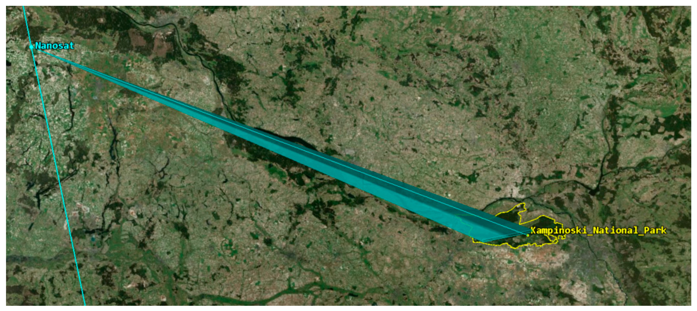
• Observation time (pass over the Area of Interest, AOI) increases with swath width and decreases with the rise in orbital velocity, which in turn, depends on orbital altitude;
• The duration of the satellite’s flight over the given area is directly related to the angle of inclination of the trajectory in reference to the equator θ and the swath width L.

The conducted analyses allow for the determination that the flight duration of 13.256 s (and hence, the possibility to make only five passes over the area of interest) is not a fully satisfactory result from the operational point of view. The altitude of the orbit of 482 km was selected as a compromise between orbital stability, minimising the influence of atmospheric drag, and ensuring the appropriate resolution of imaging for the EO sensor. Due to that, research was conducted on the possibility to perform orbital manoeuvres that may potentially increase the frequency of flights over the target area, thus improving the efficiency of the mission.

4.2. Discussion of the Results of the Analysis for a Variable Fuel Weight

The analysis of Table 8 and the parameters presented there reveals the following: data show that satellites of a similar weight with chemical propulsion systems, e.g., monopropellants (those that use hydrazine or AF-M315E), may achieve specific impulses in the range of 190–255 s. For small satellites (CubeSat and NanoSat), a realistic specific impulse for the fuel weight from 0.3 kg to 0.7 kg is in the range of 200–250 s, depending on the propulsion type. Specific impulse (I_sp) increases with the increasing weight of fuel, thus optimising its use. The typical values for these types of systems in CubeSat and NanoSat satellites may reach 200–255 s for the specific impulse.

In order to maximise the operational efficiency of nanosatellites, it may be necessary to consider the types of fuel. For example, hydrazine, and its environmentally friendly substitute LMP-103S, are perfect for precise orbital manoeuvres thanks to their high specific impulse (220–260 s) [31]. High-test peroxide (HTP) works well in green propulsion systems due to reduced toxicity [32]. Krypton and xenon, used in ion thrusters, enable long-lasting manoeuvres at minimum fuel consumption, which is crucial in satellites, such as Starlink or GOCE [33]. The choice of fuel should be adapted to the requirements of the mission, including the precision of manoeuvres, and the duration and safety of the mission.

Conclusions:

• Higher values of specific impulse and effective exhaust velocity improve the efficiency of propulsion, enabling a larger increase in velocity at lower fuel consumption. This makes it possible to perform more demanding manoeuvres.
• Larger weight of fuel allows to achieve a larger increase in velocity, which is beneficial when planning more demanding changes of the orbit.
• The duration of the manoeuvre increases significantly with the weight of fuel, which may affect planning satellite operations, e.g., the need to store energy and the availability of the propulsion system.
• Selecting the appropriate weight of fuel and specific impulse is crucial for nanosatellite systems, to ensure the maximum efficiency of the mission while complying with energy limitations.
• There is no universally optimal fuel mass. It should be carefully selected based on specific mission requirements, such as the number of planned manoeuvres, the precision of orbital changes, and time constraints.

4.3. Discussion of the Results of the Analysis of the Possible Change in Inclination

This sub-section discusses the conclusions from the data presented in Table 9, focusing, in particular, on the key parameters, such as the initial and end weight of the satellite, increase in velocity, change in inclination, and the influence on the duration of the flight over a given area. Reducing the weight of the satellite by consuming fuel has a direct influence on the satellite’s ability to perform the manoeuvre changing the inclination. For example, as the end weight increases from 7.5 kg (for a satellite of the initial weight of 8 kg) to 14.3 kg (for the initial weight of 15 kg), one may notice that the fuel consumption increases, which offers more possibilities to change the inclination. The possible change in inclination depends on the velocity increase achieved as a result of the manoeuvre. The higher this increase, the larger the possible change in inclination. For example, for a satellite of the initial weight of 15 kg and fuel weighing 0.5 kg, the change in inclination is approx. 0.009 rad (0.54°), while for a satellite with 0.7 kg of fuel, the change in inclination is approx. 0.014 rad (0.83°). An increase in velocity is the key factor that determines the satellite’s ability to change the orbit inclination. For larger amounts of fuel, the values increase, which enables a larger change in inclination. For example, for the fuel weight of 0.5 kg, the increase in velocity is 73.17 ${\displaystyle \frac{\mathrm{m}}{\mathrm{s}}}$, while for the fuel weight of 0.7 kg, it increases to 112.52 ${\displaystyle \frac{\mathrm{m}}{\mathrm{s}}}$. The duration of the satellite’s flight over the given area also depends directly on the angle of inclination of the trajectory in reference to the equator. As this angle increases, the duration of the flight over the given area decreases. For example, for a satellite with 0.5 kg of fuel, the duration is 3.87 s, while for larger amounts of fuel (e.g., 0.7 kg), the duration is 3.29 s. Even slight changes in inclination may significantly influence the satellite’s ability to observe specific areas of the Earth. For example, although a change in inclination by 0.83° may be sufficient to improve the coverage of the target area, a larger amount of fuel will allow to adjust the satellite’s trajectory to its mission more accurately.

Improving the manoeuvring capacity of the satellite by increasing fuel consumption makes it possible to better adjust the orbit to the objectives of the mission. Effective exhaust velocity that results from the specific impulse also influences the satellite’s ability to change its orbit. Higher specific impulse means an increased exhaust velocity, which enables more efficient fuel consumption. For a satellite with the specific impulse of 220 s, effective exhaust velocity is 1867.80 ${\displaystyle \frac{\mathrm{m}}{\mathrm{s}}}$, which allows to achieve a higher increase in velocity than for a satellite with a specific impulse of 180 s, where the exhaust velocity is 1528.20 ${\displaystyle \frac{\mathrm{m}}{\mathrm{s}}}$.

In conclusion, a larger amount of fuel and higher specific impulse enable the satellite to introduce larger changes to the inclination and velocity, which is essential for adjusting the orbit to mission objectives. The duration of the satellite’s flight over the area of interest decreases with the increase in the angle of trajectory inclination, which affects the efficiency of observations.

The analysis of Table 9 revealed one anomaly. In the table, for the fuel weight of 0.35 kg, the angle of the inclination of trajectory in reference to the equator is 1.263 rad. This is a relatively large angle, which influences the satellite’s velocity in reference to the surface of the Earth. The angle corresponds to orbit inclination, which means that the satellite moves more diagonally in reference to Earth’s surface, which reduces the velocity of the projection of its movement on the surface of our planet. The value of cosθ decreases with the increase in the angle of inclination. As a result, the satellite’s velocity in reference to the surface of the Earth diminishes. In this specific case, this means that only approx. 22.6% of the total velocity of the satellite (7800 ${\displaystyle \frac{\mathrm{m}}{\mathrm{s}}}$) is translated into motion in reference to the surface of the Earth. This significantly reduces the velocity relative to the Earth’s surface, which prolongs the duration of flight over a given area. In this case, the flight duration is 8.22 s, being significantly longer than the neighbouring options, where the angle of inclination is smaller and the velocity relative to the surface of the Earth is higher. It results in an extended duration of flight over the given area, which may be beneficial for certain missions, e.g., for observation purposes, where it is required for the satellite to spend more time over a specific area. However, the need to process data and maintain contact with the satellite for a longer time during such a flight may generate increased energy costs.

Through the comparison of the results of the conducted analysis of the change in orbit inclination with examples of orbital manoeuvres provided in the literature, one may notice significant differences in the required ∆v, duration of the manoeuvre, and fuel consumption. An example presented in the literature, where changing the inclination by 2.17° requires ∆v = 4.22 ${\displaystyle \frac{\mathrm{k}\mathrm{m}}{\mathrm{s}}}$, points to high energy requirements for short impulsive manoeuvres [7]. In a different case, at low thrust, changing the inclination by 5.6° required ∆v = 1.18, but at the expense of the long duration of the manoeuvre (54 days) and consuming 25.8 kg of fuel by a satellite of the initial weight of 367 kg [34].

Conclusions:

• The ability to change orbital inclination is strongly dependent on both fuel mass and specific impulse. Even a slight increase in available ∆v allows for more advanced manoeuvres.
• An increase in specific impulse by 10 s results in an increase in exhaust gas velocity by approximately 85 ${\displaystyle \frac{\mathrm{m}}{\mathrm{s}}}$, improving fuel utilisation efficiency.
• Even small changes in inclination (≈0.5–0.8°) may significantly influence the coverage of the target area.
• A longer duration of flight over the given area may be beneficial for observation missions, but it requires more precise manoeuvres.
• The optimum orbit should take into account the compromise between the amount of fuel, efficiency of the manoeuvre, and the required duration of the flight over the area.

4.4. Discussion of the Results of the Analysis of the Weight of Fuel Necessary to Perform the Hohmann Transfer

Now let us move on to the conclusions from the data provided in Table 10, taking into account specific key parameters, such as the initial and end weight of the satellite, increase in velocity, as well as the amount of fuel necessary to perform the Hohmann transfer. The influence of the initial weight and amount of fuel should be analysed. The amount of fuel required to perform the manoeuvre increases with the increasing initial weight of the satellite. The analysis reveals that for a satellite of the initial weight of 8 kg, the amount of fuel necessary to change the orbit from 482 km to 550 km is approx. 0.194 kg, whereas a satellite of the initial weight of 15 kg requires 0.300 kg of fuel to perform the same orbital transfer. Then, the increase in velocity was analysed. The values of ∆v₁ and ∆v₂ are essential to calculate the amount of energy that must be provided to change the orbit. In the calculations, the increases in velocity remain relatively stable for different weights of the satellite, which means that the increase in weight influences, first of all, the necessary amount of fuel. The total increase in velocity is approx. 37.56 ${\displaystyle \frac{\mathrm{m}}{\mathrm{s}}}$, which is a relatively low ∆v, considering the analysed change in the altitude of the orbit. Specific impulse (I_sp) is another key parameter that influences the efficiency of fuel consumption. For the specific impulse of 180 s, the effective exhaust velocity is 1527.69 ${\displaystyle \frac{\mathrm{m}}{\mathrm{s}}}$. A higher specific impulse means lower fuel consumption at the same ∆v, which enables to use the resources of the satellite more economically. The semi-major axis of the transfer orbit (which is approx. 6887 km in the analysis) influences the velocity in the perigee and apogee of the transfer orbit. These values indicate the difference in velocities that the satellite must achieve to perform a successful transfer. In conclusion, a larger amount of fuel allows to perform larger manoeuvres to change the orbit altitude. However, even for a relatively small increase in velocity (37.56 ${\displaystyle \frac{\mathrm{m}}{\mathrm{s}}}$), the difference in the required amount of fuel is significant for heavier satellites. A higher specific impulse means lower fuel consumption, which is crucial for satellite missions where saving weight is important. The value of 1527.69 ${\displaystyle \frac{\mathrm{m}}{\mathrm{s}}}$ of effective exhaust velocity means that every change in ∆v requires a significant amount of fuel. The analysis reveals that the increases in velocity must be calculated precisely in order to avoid situations when the planned manoeuvres will become impossible with the available resources. Even slight differences in ∆v may have a great influence on mission planning. Efficient fuel management is crucial, in particular for missions that require multiple manoeuvres. The possibility to change the orbit with limited resources is important for the achievement of the satellite’s long-term goals, such as the observation of the Earth or adjusting the orbit to changing needs. In conclusion, it is possible to perform the Hohmann transfer in order to change the altitude of the orbit, yet only with correct fuel management and a proper understanding of the influence of specific impulse on propulsion efficiency.

The results of the analysis reveal the total increase in velocity ∆v_total = 37.56 ${\displaystyle \frac{\mathrm{m}}{\mathrm{s}}}$. These are significantly lower values in comparison, for example, to the Hohmann transfer, such as the example provided in [35], where the first increase in velocity was ∆v₁ = 2.25 ${\displaystyle \frac{\mathrm{k}\mathrm{m}}{\mathrm{s}}}$, the second increase was ∆v₂ = 1.46 ${\displaystyle \frac{\mathrm{k}\mathrm{m}}{\mathrm{s}}}$, and the total increase was ∆v_total = 3.71 ${\displaystyle \frac{\mathrm{k}\mathrm{m}}{\mathrm{s}}}$. The duration of the Hohmann transfer was 3 h and 56 min, which also differs from the impulsive nature of the analysis, where the manoeuvres only take seconds. Similarly, for the data of SpaceX [36], the first impulse for the F9-25 Thiacom 8 mission was ∆v₁ = 2.25 ${\displaystyle \frac{\mathrm{k}\mathrm{m}}{\mathrm{s}}}$, while for F9-70 Nusantara ∆v₁ = 2.74 ${\displaystyle \frac{\mathrm{k}\mathrm{m}}{\mathrm{s}}}$, with the manoeuvre lasting for approximately 5 h.

The differences mainly result from the smaller scale of the orbit changes in the analysis and the differences in the weight and characteristics of the satellites, which influence both the required increases in velocity, and the duration of the manoeuvres.

In the context of the Hohmann transfer, it is possible to apply simple optimisation methods, such as minimising fuel consumption while maintaining the required parameters of orbital transfer. An example may be selecting the specific impulse and ∆v so as to achieve the fuel efficiency within the limits of the available resources. It is recommended for future analyses to apply such optimisation methods that might additionally improve the efficiency of the manoeuvre.

Conclusions:

• The weight of the necessary fuel increases with the increase in the initial weight of the satellite. Heavier satellites require more fuel to generate the same increase in velocity.
• Higher specific impulse leads to a reduction in the required amount of fuel. This results from a higher effective exhaust velocity, which improves the efficiency of the thruster.
• Higher effective exhaust velocity leads to a reduction in the required amount of fuel.
• The value of the total increase in velocity remains constant, regardless of the weight of the satellite or other parameters, since it is determined by the geometry and altitude of the orbits.
• Higher values of specific impulse lead to a significant reduction in the required amount of fuel; an increase in specific impulse by 10 s allows for a reduction in fuel demand by approximately 15 g, which is essential for missions with limited weight resources, such as nanosatellites.
• The optimum choice for satellites weighing up to 15 kg are propulsion systems with a high specific impulse to minimise the weight of fuel.

4.5. Discussion of the Comparative Analysis of Hohmann Transfers and Inclination Change Maneuvers in Terms of Energy Requirements and Mission Efficiency

Based on the previous analysis of both types of manoeuvres, a qualitative comparison was conducted to evaluate the trade-offs between the velocity increment requirement (Δv) and operational benefits.

Table 13. Qualitative comparison of Hohmann transfers and inclination change manoeuvres in the context of nanosatellite missions.

Type of Orbital Manoeuvre	Demand for Speed Change	Impact on Flight Time and AOI	Flexibility of Land Cover	Comments
Hohmann manoeuvre (in one plane)	Low ($~50–100{\displaystyle \frac{\mathrm{m}}{\mathrm{s}}}$)	Slightly extended (due to lower velocity in higher orbit)	Restricted (ground track unchanged)	Simple, energy-efficient, extends observation time
Change in inclinations	Very high ($>100{\displaystyle \frac{\mathrm{m}}{\mathrm{s}}}$ per °)	Varies (depending on direction and extent of change)	High (change in geometry of ground track)	Costly, justified only by the requirements of the specific mission

presents the main characteristics of each strategy in the context of constraints typical for nanosatellite missions.

The analysis included the Hohmann transfer as one of the realistic strategies for orbital altitude changes in nanosatellite missions. This manoeuvre is widely used due to its simplicity, low energy cost, and feasibility with limited fuel resources, making it particularly suitable for small satellite platforms. Changing orbital altitude directly affects the satellite’s orbital velocity; the higher the orbit, the lower the velocity, which translates into an extended overpass time over the area of interest (AOI). This enables a longer observation of a selected region during a single pass.

An alternative strategy is the inclination change manoeuvre, which allows for achieving more favourable geographical coverage by modifying the orbital path geometry. However, it should be noted that this type of manoeuvre requires a very high velocity change (Δv), often exceeding 100 ${\displaystyle \frac{\mathrm{m}}{\mathrm{s}}}$ for each degree of inclination change. In the context of nanosatellites, which have limited fuel and energy budgets, performing such a maneuver can be challenging.

For this reason, this study presents a qualitative comparison of both manoeuvring strategies, highlighting the trade-off between energy efficiency and mission effectiveness. In many cases, the Hohmann transfer proves to be a more cost-effective solution, offering significant operational benefits, such as extended observation time at a lower energy cost. On the other hand, the inclination change manoeuvre, despite its higher costs, may be justified for missions requiring a precise coverage of specific geographical areas, particularly those with irregular distributions.

4.6. Discussion of the Results of the Analysis of the Energy Required to Tilt the Satellite by a Specific Angle

This sub-section focuses on the interpretation of the results presented in Table 11. The energy consumed by reaction wheels is linearly proportional to the duration of the manoeuvre. This results from the assumed constant power consumption of 0.45 W. For small tilt angles, such as 1°, energy consumption is very low (0.09 J), whereas for the maximum angle of 30°, it increases to 2.70 J. The duration of the manoeuvre is proportional to the tilt angle and ranges from 0.2 s (1°) to 6.0 (30°) at a constant rotation rate of 5 ${\displaystyle \frac{°}{\mathrm{s}}}$.

These values are realistic and consistent with the adopted design assumptions. For the charging power of 70 W, the charging time remains very short, ranging from 0.0013 s for the 1°$\mathrm{a}\mathrm{n}\mathrm{g}\mathrm{l}\mathrm{e}\mathrm{t}\mathrm{o}$ 0.0386 s for the angle of 30°. These results suggest that the power system of the satellite is able to regenerate fast after performing the manoeuvre, which has a positive influence on its operational capacity. In conclusion, the conducted calculations and analysis demonstrate that the M6P satellite is optimised mechanically and in terms of energy to perform tilt manoeuvres within a wide range of angles. Thanks to the efficient power recovery system and low energy consumption for manoeuvres, the satellite is well adapted to perform missions that require a precise management of its spatial orientation.

Conclusions:

• The analysis revealed that the power system of the nanosatellite with the selected parameters is suitable for performing short tilt manoeuvres. Thanks to the high charging power of the solar panels equal to 70 W, energy recovery time is less than 0.04 s; the satellite is able to quickly recover the energy required for further manoeuvres.
• Assuming that regular tilt manoeuvres of a maximum angle of 30° are performed, the satellite may perform these operations with a minimum influence on the availability of power, which is crucial for missions that require a large number of spot observations. Reaction manoeuvres using the reaction wheels are highly energy-efficient; even a full assumed pivot (30°) requires only 2.7 J.
• The results of the analysis suggest that the M6P satellite may be used in intensive observational operations, such as the monitoring of selected areas of the Earth, without the risk of running out of energy. The short charging time after each manoeuvre allows to increase the frequency of operational activities.

The analysis based on the obtained results makes it possible to analyse in detail the operational capacity of the nanosatellite dedicated to acquiring images of the given region, with the characteristics provided in Section 2 (e.g., the Kampinos Forest, of the surface area of approx. 385 km^2, situated on 52° latitude). The analysis focused on several key aspects: Propulsion efficiency, the required amount of fuel, the optimisation of the satellite’s orientation, and the influence of orbital parameters on the data acquisition capacity.

Conclusions concerning the propulsion and fuel:

The analysis demonstrates that satellites of different weights and specific impulses are characterised by various fuel consumption efficiency. Higher specific impulse I_sp enables a more efficient use of the fuel, which is particularly important for nanosatellite missions as their resources are limited. For example, a satellite of the initial weight of 15 kg needs approx. 0.3 kg of fuel at the specific impulse I_sp = 230 s to change the orbit from 482 km to 550 km. An increase in the initial weight leads to a growing demand for fuel, which limits the manoeuvring capacity of the satellite. This results from the fact that a larger weight requires a larger increase in velocity ∆v, which involves higher energy losses.

Conclusions concerning the swath width and flight duration:

The swath width depends mainly on the quality of the sensor installed on the board of the satellite. Analyses reveal that for a satellite weighing 15 kg, the swath width is approx. 19.4 km. This is sufficient to provide an effective coverage of areas similar in size to Kampinos National Park during a single flight. However, it should be noted that a single flight will almost completely cover the area of the Kampinos National Park. Full coverage of the area requires two flights, since the scenes should partly overlap in order to ensure the consistency of observational data and an accurate representation of the terrain. However, for heavier satellites, the swath width may increase to 21 km, which involves higher costs of weight and of fuel consumption. A satellite equipped with a sensor that offers the swath width of 19.4 km seems to be sufficient for a mission that focuses on one region.

Conclusions concerning the change in inclination:

Although changing the orbit inclination may be essential in certain missions, the analysis revealed that in the case discussed here, it is rather not cost effective. Even a slight change in inclination (0.47° for a satellite with the initial weight of 15 kg and 0.5 kg of fuel) requires a large amount of fuel, which affects the overall efficiency of the mission. Considering that such change in inclination does not significantly improve the coverage of the target area, it seems more reasonable to focus on other operational areas. For example, one might use the change in the orientation of the satellite and sensor to prolong the duration of observations (by manoeuvres performed with the use of reaction wheels that consume power). Instead of changing the inclination, it is worth investing the fuel resources in regular manoeuvres to increase the altitude of the orbit, as they are more efficient and enable to extend the lifespan of the mission. Manoeuvres changing the inclination should be considered only in situations when they are absolutely necessary to achieve the goals of the mission.

Conclusions concerning the power system and orientation manoeuvres:

Using reaction wheels to precisely set the orientation of the satellite in reference to the selected area allows to extend the duration of observations. The analyses revealed that the M6P satellite by NanoAvionics, of the weight of 4.5 kg (without fuel) and the dimensions of 0.1 m × 0.2 m × 0.3 m, is optimised for short orientation manoeuvres. At the solar panel charging power of 70 W, the time needed for power regeneration after the manoeuvre is minimal, ranging from 0.0013 s (for the tilt angle of 1°) to 0.0386 s (for the angle of 30°). This enables the satellite’s power system to support intensive observation operations, even if a large number of tilt manoeuvres are performed.

4.7. Discussion of the Results of the Selection of the Optimum Nanosatellite Dedicated to Maximise the Specific Operational Task

The analysis of Table 12 refers to various types of satellites in terms of their initial weight, fuel weight, specific impulse, and frontal surface. Some operational parameters, including the drag force, orbital energy loss, and the resulting decrease in altitude were also taken into account. The aim of the analysis was to select the optimum nanosatellite that will balance fuel efficiency, orbital stability, and the operational complexity of the mission. Satellites of a low initial weight, ranging from 8 kg to 10 kg are characterised by relatively low drag thanks to their small frontal surface of 0.02 m². This translates into a low drag force of 0.00000135 N, which, in turn, results in reduced orbital energy losses and a moderate decrease in altitude of approx. 2 km per half a year. However, in spite of low fuel consumption (approx. 0.3 kg), nanosatellites of such low weight may have limited operational capacity, including fewer telescopes on board or limited fuel capacity, which reduces their ability to perform a larger number of adjustment manoeuvres. For satellites of medium weight, from 11 kg to 15 kg, the frontal surface increases to 0.03 m², which leads to a stronger drag force of 0.00000203 N. In spite of larger energy losses (approx. 40960 J) and drops of altitude of about 2 km, nanosatellites in this weight category offer a better balance between efficiency and functional capacity. Higher weight allows them to carry more fuel, which improves the flexibility of the mission. For example, a nanosatellite weighing 15 kg, with a specific impulse of 220 s, uses in total, approx. 0.442 of fuel in six months. This is acceptable in the context of long-term orbital missions. Thanks to their moderate fuel consumption and better orbital stability, nanosatellites in this weight category seem to be more universal. Finally, heavy satellites that weigh from 16 kg to 18 kg are characterised by a larger frontal surface of approx. 0.04 m², which causes a further increase in the drag forces to 0.00000270 N. Increased orbital energy losses (54613.72 J) and drops in altitude exceeding 2.4 km in six months require higher fuel consumption. A satellite that weight 18 kg uses as much as 0.488 kg of fuel. In spite of their great operational capacity, nanosatellites in this category are less fuel efficient, and their weight may limit the viability of an orbit launch.

Conclusions:

• Although heavier satellites offer more advanced functional capabilities, their fuel requirements are increasing. Based on the data analysis, one may assume that the optimum configuration is a satellite weighing 5 kg. This range of weight ensures a proper balance between the capacity and orbital stability, while, at the same time, enabling the installation of an advanced sensor.
• The specific impulse of 220 s guarantees high fuel efficiency with moderate technical requirements. Higher values of the specific impulse might reduce fuel consumption, yet they are less cost-efficient for satellites in this weight category.
• The weight of fuel of 0.5 kg is perfectly suitable for missions lasting up to six months, provided that the amount of fuel spent on manoeuvres to adjust the orbit is moderate. This amount allows six manoeuvres to be performed, increasing the altitude of the orbit by 643 m, which effectively prevents orbit degradation.
• The drag force increases in proportion to the face area, which in turn, scales with the mass of the satellite. The frontal surface of 0.02 m² that is determined by the satellite’s dimensions minimises the influence of drag, which translates into lower energy losses and a more stable trajectory.

This type of nanosatellite offers a compromise between fuel efficiency and operational capacity. The fuel consumption per six months, taking into account only the manoeuvre of increasing orbit altitude, is 0.154 kg, which enables efficient resource management while maintaining orbital stability. The selection of the nanosatellite with the parameters presented above minimises both the energy losses and the complexity of the mission, while ensuring sufficient flexibility for potential modifications of the orbit.

5. Conclusions

The conducted analyses provided a comprehensive knowledge of the operational capacity of the nanosatellite dedicated to capturing images of a selected area. The research focused on several key aspects, including propulsion efficiency, the optimum selection of the weight of satellite and of fuel, swath width, and the influence of orbital parameters on the nanosatellite’s ability to perform observation missions effectively. In particular, it was demonstrated that the selection of the appropriate propulsion system is of key importance for improving fuel efficiency, which enables to perform more complex orbital manoeuvres while, at the same time, reducing fuel consumption.

The analysis revealed that the precise planning of manoeuvres such as, for example, changing the altitude of the orbit by means of the Hohmann transfer, allows for the minimisation of fuel costs and maintaining orbital stability. The conducted research also enabled to assess the influence of the satellite’s weight on the swath width and the duration of flight over the target area. The results demonstrated that a higher weight of the satellite, with correctly selected sensor parameters, enables an increase in the swath width, which is important from the point of view of missions that are aimed at monitoring large areas. Furthermore, the analysis of the flight duration highlighted the fact that the key factor is the inclination of the satellite’s trajectory in reference to the equator, as it influences the actual velocity relative to the Earth’s surface, and thus, the efficiency of data acquisition. The analysis of inclination changing manoeuvres revealed their high energy and fuel costs for nanosatellites. This provides an inspiration to search for alternative solutions. In this context, the authors proposed to use manoeuvres to change the orientation. They are performed with the use of reaction wheels that consume power resources instead of fuel and at the same time enable prolonging the duration of the observation of the area of interest. The power system of the nanosatellite was considered to be well-optimised in terms of intensive orientation-changing operations. Thanks to that, the satellite may perform short tilting manoeuvres that have only a slight influence on the availability of energy resources.

The obtained results provide a solid basis for further research. It was demonstrated that satellites in the nano and nano+ classes may be effectively used in various missions. Although this study does not introduce new equations or algorithms, it provides an evaluation of existing orbital manoeuvres from the perspective of their application to nanosatellite missions, supporting designers in making decisions at an early stage of mission planning. Future research projects should be aimed at the optimisation of orbital manoeuvres, with particular focus on the strategies that minimise fuel and energy consumption in order to improve the efficiency of nanosatellites and to enable the realisation of more complex, long-term missions in the dynamically changing orbital conditions. In the future, it is also worth considering the application of optimisation algorithms that will enable the more precise planning of orbital manoeuvres by minimising fuel and energy consumption and maximising the operational efficiency of nanosatellites. The research results highlight the importance of precise planning and the optimisation of mission parameters, which is crucial for the maximisation of the efficiency of nanosatellites when resources are limited.

References

1. Roshan, S.; Raunak, S.; Kaushik, D. Constellation Design of Remote Sensing Small Satellite for Infrastructure Monitoring in India. arXiv 2021, arXiv:2107.09253. [Google Scholar]
2. Luo, Q.; Peng, W.; Wu, G.; Xiao, Y. Orbital Maneuver Optimization of Earth Observation Satellites Using an Adaptive Differential Evolution Algorithm. Remote Sens. 2022, 14, 1966. [Google Scholar] [CrossRef]
3. Banks, B.A.; Miller, S.K.; de Groh, K.K. Low Earth Orbital Atomic Oxygen Interactions with Materials. MRS Proc. 2004, 851, 426–437. [Google Scholar] [CrossRef]
4. It’s Some Kind of Space. Available online: https://www.youtube.com/watch?v=DvO3FLcLC88&t=1360s (accessed on 17 January 2024).
5. Nunes Vaz, B.; Bertachini De Almeida Prado, A.F. Sub-Optimal Orbital Maneuvers for Artificial Satellites. WSEAS Trans. Appl. Theor. Mech. 2008, 3, 769. Available online: https://www.wseas.us/e-library/transactions/mechanics/2008/28-469.pdf (accessed on 10 January 2025).
6. Butikov, E.I. Orbital maneuvers and space rendezvous. Adv. Space Res. 2015, 56, 2582–2594. [Google Scholar] [CrossRef]
7. Curtis, H.D. Orbital Mechanics for Engineering Students, 4th ed.; Elsevier Ltd.: Amsterdam, The Netherlands, 2020. [Google Scholar]
8. Chen, Y.; Mahalec, V.; Chen, Y.; He, R.; Liu, X. Optimal Satellite Orbit Design for Prioritized Multiple Targets with Threshold Observation Time Using Self-Adaptive Differential Evolution. J. Aerosp. Eng. 2015, 28, 04014066. [Google Scholar] [CrossRef]
9. Savitri, T.; Kim, Y.; Jo, S.; Bang, H. Satellite Constellation Orbit Design Optimization with Combined Genetic Algorithm and Semianalytical Approach. Int. J. Aerosp. Eng. 2017, 2017, 1–17. [Google Scholar] [CrossRef]
10. Sengupta, P.; Vadali, S.R.; Alfriend, K.T. Satellite Orbit Design and Maintenance for Terrestrial Coverage. J. Spacecr. Rocket. 2010, 47, 177–187. [Google Scholar] [CrossRef]
11. Graham, K.F.; Rao, A.V. Minimum-Time Trajectory Optimization of Low-Thrust Earth-Orbit Transfers with Eclipsing. J. Spacecr. Rocket. 2016, 53, 289–303. [Google Scholar] [CrossRef]
12. Zhang, C.; Topputo, F.; Bernelli-Zazzera, F.; Zhao, Y.S. Low-Thrust Minimum-Fuel Optimization in the Circular Restricted Three-Body Problem. J. Guid. Control. Dyn. 2015, 38, 1501–1510. [Google Scholar] [CrossRef]
13. Wang, Z.; Grant, M.J. Optimization of Minimum-Time Low-Thrust Transfers Using Convex Programming. J. Spacecr. Rocket. 2017, 55, 586–598. [Google Scholar] [CrossRef]
14. Sadegh Mohammadi, M.; Naghash, A. Robust optimization of impulsive orbit transfers under actuation uncertainties. Aerosp. Sci. Technol. 2019, 85, 246–258. [Google Scholar] [CrossRef]
15. Morante, D.; Sanjurjo-Rivo, M.; Soler, M.; Sánchez-Pérez, J.M. Hybrid multi-objective orbit-raising optimization with operational constraints. Acta Astronaut. 2020, 175, 447–461. [Google Scholar] [CrossRef]
16. Cheng, L.; Wang, Z.; Jiang, F.; Zhou, C. Real-Time Optimal Control for Spacecraft Orbit Transfer via Multiscale Deep Neural Networks. IEEE Trans. Aerosp. Electron. Syst. 2018, 55, 2436–2450. [Google Scholar] [CrossRef]
17. Song, Z.; Chen, X.; Luo, X.; Wang, M.; Dai, G. Multi-objective optimization of agile satellite orbit design. Adv. Space Res. 2018, 62, 3053–3064. [Google Scholar] [CrossRef]
18. Appel, L.; Guelman, M.; Mishne, D. Optimization of satellite constellation reconfiguration maneuvers. Acta Astronaut. 2014, 99, 166–174. [Google Scholar] [CrossRef]
19. Paek, S.W.; Kim, S.; de Weck, O. Optimization of Reconfigurable Satellite Constellations Using Simulated Annealing and Genetic Algorithm. Sensors 2019, 19, 765. [Google Scholar] [CrossRef]
20. Sarno, S.; Guo, J.; D’Errico, M.; Gill, E. A guidance approach to satellite formation reconfiguration based on convex optimization and genetic algorithms. Adv. Space Res. 2020, 65, 2003–2017. [Google Scholar] [CrossRef]
21. He, X.; Li, H.; Yang, L.; Zhao, J. Reconfigurable Satellite Constellation Design for Disaster Monitoring Using Physical Programming. Int. J. Aerosp. Eng. 2020, 2020, 8813685. [Google Scholar] [CrossRef]
22. Wang, X.; Zhang, H.; Bai, S.; Yue, Y. Design of agile satellite constellation based on hybrid-resampling particle swarm optimization method. Acta Astronaut. 2021, 178, 595–605. [Google Scholar] [CrossRef]
23. Soleymani, M.; Fakoor, M.; Bakhtiari, M. Optimal mission planning of the reconfiguration process of satellite constellations through orbital maneuvers: A novel technical framework. Adv. Space Res. 2019, 63, 3369–3384. [Google Scholar] [CrossRef]
24. Hu, J.; Huang, H.; Yang, L.; Zhu, Y. A multi-objective optimization framework of constellation design for emergency observation. Adv. Space Res. 2021, 67, 531–545. [Google Scholar] [CrossRef]
25. Bate, R.; Mueller, D.; White, E.; Saylor, W. Fundamentals of Astrodynamics, 2nd ed.; Dover Publications: Garden City, NY, USA, 2020. [Google Scholar]
26. Sutton, G.P.; Biblarz, O. Rocket Propulsion Elements, 9th ed.; Wiley: Hoboken, NJ, USA, 2017. [Google Scholar]
27. Wertz, J.R. Mission Geometry; Orbit and Constellation Design and Management: Spacecraft Orbit and Attitude Systems; Springer: Berlin/Heidelberg, Germany, 2001. [Google Scholar]
28. Wertz, J.R.; Larson, W.J. Space Mission Analysis and Design, 3rd ed.; Space Technology Library; Springer: Berlin/Heidelberg, Germany, 1999. [Google Scholar]
29. MultiScape100 CIS Product. Available online: https://simera-sense.com/products/multiscape100/ (accessed on 15 June 2024).
30. CubeSat 6U CubeSat/ Nanosatellite M6P. Available online: https://nanoavionics.com/small-satellite-buses/6u-cubesat-nanosatellite-m6p/ (accessed on 6 October 2024).
31. Sentinel-2 Operations. Available online: https://www.esa.int/Enabling_Support/Operations/Sentinel-2_operations (accessed on 10 January 2025).
32. Successful Demonstration of Polish Missile Technologies. Flight of the ILR-33 “Amber” Missile”. Available online: https://ilot.lukasiewicz.gov.pl/udana-demonstracja-polskich-technologii-rakietowych-lot-rakiety-ilr-33-bursztyn/ (accessed on 10 January 2025).
33. Why Do Starlink Satellites Use Krypton for Electric Propulsion Instead of Xenon? Available online: https://chimniii.com/news/Technology/Technology-Starlink-why-do-starlink-satellites-use-krypton-for-electric-propulsion-instead-of-xenon.html (accessed on 10 January 2025).
34. Ruggiero, A.; Pergola, S.; Marcuccio, S.; Andrenucci, M. Low-Thrust Maneuvers for the Efficient Correction of Orbital Elements, IEPC-2011-102. In Proceedings of the 32nd International Electric Propulsion Conference, Wiesbaden, Germany, 11–15 September 2011. [Google Scholar]
35. Derfel, G. From Orbit to Orbit, Institute of Physics, Lodz University of Technology. Available online: https://www.deltami.edu.pl/media/articles/2020/08/delta-2020-08-z-orbity-na-orbite.pdf (accessed on 13 January 2025).
36. Michael, J.R.; Perkins, J. SpaceX Rocket Data Satisfies Elementary Hohmann Transfer Formula. Phys. Educ. 2020, 55, 025011. [Google Scholar]
Figure 1. Orbital coordinate system used for satellite motion analysis. Created based on [4]. (a) Representation of a satellite moving in an Earth orbit with indications of radial, normal, and “along-track” directions at a selected point of the orbit. (b) Directions of engine alignment during orbital manoeuvres.
Applsci 15 05360 g001
Figure 2. Hohmann transfer, a diagram. Created based on [7]. (1) Central body; (2) Internal circular orbit of radius r1; (3) External circular orbit of radius r2; Points A and B represent the periapsis and apoapsis of the transfer ellipse.
Applsci 15 05360 g002
Figure 3. Manoeuvre changing the orbital plane—diagram. Created based on [7]. (a) Two non-coplanar orbits around F. (1) Initial orbit; (2) Final orbit. (b) View along the line of intersection of two orbital planes. (1) Plane of the initial orbit; (2) Plane of the final orbit.
Applsci 15 05360 g003
Figure 4. Impulsive manoeuvre of changing the orbit plane in the apocentre—diagram. Created based on [7]. (1) Initial elliptical orbit; (2) Final elliptical orbit.
Applsci 15 05360 g004
Figure 5. Visualisation of the range of the nanosatellite observations during a single flight over Kampinos National Park. (Source: STK 12.7.1).
Applsci 15 05360 g005
Figure 6. Simulation of the inclination change manoeuvre performed in the STK 12.7.1 environment. The green line shows the initial orbit with an inclination of 97°, while the magenta line corresponds to the modified orbit with an inclination of 96.28°. (a) 3D visualisation of the manoeuvre of changing the inclination of the orbit; (b) 2D visualisation of the manoeuvre of changing the inclination of the orbit.
Applsci 15 05360 g006
Figure 7. Visualisation of the Hohmann transfer. The green line represents the initial circular orbit at an altitude of 482 km, while the blue line corresponds to the final circular orbit at an altitude of 550 km. (Source: STK 12.7.1).
Applsci 15 05360 g007
Figure 8. Visualisation of the tilt of the sensor with the satellite platform and of the coverage of Kampinos National Park. (Source: STK 12.7.1).
Applsci 15 05360 g008