A Time-Segmented SAI-Krylov Subspace Approach for Large-Scale Transient Electromagnetic Forward Modeling

Abstract

After nearly two decades of development, transient electromagnetic (TEM) 3D forward modeling technology has significantly improved both numerical precision and computational efficiency, primarily through advancements in mesh generation and the optimization of linear equation solvers. However, the dominant approach still relies on direct solvers, which require substantial memory and complicate the modeling of electromagnetic responses in large-scale models. This paper proposes a new method for solving large-scale TEM responses, building on previous studies. The TEM response is expressed as a matrix exponential function with an analytic initial field for a step-off source, which can be efficiently solved using the Shift-and-Invert Krylov (SAI-Krylov) subspace method. The Arnoldi algorithm is used to construct the orthogonal basis for the Krylov subspace, and the preconditioned conjugate gradient (PCG) method is applied to solve large-scale linear equations. The paper further explores how dividing the off-time and optimizing parameters for each time interval can enhance computational efficiency. The numerical results show that this parameter optimization strategy reduces the iteration count of the PCG method, improving efficiency by a factor of 5 compared to conventional iterative methods. Additionally, the proposed method outperforms direct solvers for large-scale model calculations. Conventional approaches require numerous matrix factorizations and thousands of back-substitutions, whereas the proposed method only solves about 300 linear equations. The accuracy of the approach is validated using 1D and 3D models, and the propagation characteristics of the TEM field are studied in large-scale models.

1. Introduction

TEM has undergone rapid development and achieved significant progress, becoming widely used in various fields such as mineral exploration [1,2,3,4], hydrogeophysical exploration [5,6,7], tunnel prediction [8,9], and more [10,11]. TEM forward modeling serves as the foundation for data interpretation and 3D inversion. As the demand for detailed detection and data interpretation continues to grow, the need for 3D large-scale forward modeling has become increasingly urgent [12].

Currently, TEM 3D forward modeling methods can be broadly categorized into three types: the finite difference method [13,14,15,16], the implicit time-step method [17,18,19,20,21], and the Krylov subspace method [22,23,24,25,26,27]. Among these methods, the implicit time-step and Krylov subspace methods typically employ direct solvers to simulate the TEM response for small- to medium-scale models. However, simulating the electromagnetic response of large-scale models presents considerable challenges in terms of memory usage [28]. While the iterative method based on the implicit time-step can also address large-scale models, its computational efficiency requires further improvement, and selecting the optimal time step remains a challenging task [17,19,29]. The three-dimensional finite difference method in the time domain does not require solving linear equations, but careful selection of the time step and mesh size is still needed to prevent numerical overflow due to numerical dispersion [14,15,16].

In recent years, the Krylov subspace method has made significant advancements compared to the traditional implicit time-step method. Hochbruck and Lubich and Van and Hochbruck addressed the slow convergence issue of the SAI-Krylov subspace algorithm, proving that the Krylov subspace method always approximates an exponential function with a superlinear convergence rate, independent of mesh size [30,31]. Additionally, Börner et al. highlighted that the Krylov subspace method outperforms other methods in terms of convergence [25]. Furthermore, the Krylov subspace method eliminates the need to select a time step, enabling the calculation of the electromagnetic response at any point in the off-time period [25,26,27]. Zhou et al. demonstrated fast TEM forward modeling using the SAI-Krylov subspace method [26]. Compared with the rational Krylov subspace algorithm, the SAI-Krylov subspace method offers faster computational efficiency [32]. Based on these advancements, this paper proposes a new method for solving TEM responses using the SAI-Krylov subspace method. However, for large-scale models with millions to even billions of unknowns, the combined computational strategy of SAI-Krylov and direct solvers is relatively inefficient.

Compared to the direct solvers, the iterative method only requires storing the sparse matrix and a small number of vector elements [17]. The primary computational effort in the iterative process involves multiplying the coefficient matrix by the vector. The PCG method is a highly effective optimization technique that only requires first-order derivative information. This method not only addresses the slow convergence of the steepest descent method but also avoids the limitations of the Newton method, which requires storing and calculating the Hessian matrix [33]. The PCG method is well suited for solving large linear equations and is also applicable to large nonlinear problems. Compared to other iterative methods, the PCG method offers clear advantages in accuracy and efficiency when using the same initial value and error threshold [34].

As a classic iterative method, the PCG technique has been widely employed in electromagnetic numerical simulations. Wu and Xu applied the conjugate gradient method to three-dimensional resistivity inversion, achieving satisfactory results [35]. Later, Wu and Wang used the conjugate gradient method for three-dimensional finite element forward modeling of resistivity, which not only reduced memory usage but also improved the computational performance of forward modeling [36]. In the field of TEM forward modeling, Li et al. applied the PCG method to solve electromagnetic fields in the frequency domain and obtained time-domain responses using the Gaver–Stehfest algorithm [33]. Um et al. employed the PCG method to simulate large-scale electromagnetic responses based on unstructured meshes and further explored its application in finite element forward modeling [17]. In the study of CSEM 3D inversion, Peng et al. used the PCG method to solve the normal equation in each iteration, avoiding the explicit solution and storage of the sensitivity matrix, thus reducing computational cost and achieving satisfactory 3D inversion results [37]. Given the unique advantages of the PCG method, it has also been widely applied in 3D forward and inverse modeling in seismic exploration [38,39,40].

In summary, this study combines the PCG method with the SAI-Krylov subspace technique to solve the TEM response for large-scale models. By dividing the off-time and analyzing and selecting optimization parameters, the computing performance of the proposed method is further enhanced.

The main content of this paper is segmented into three parts. The first part introduces the application of the SAI-Krylov subspace method and the PCG method in TEM 3D finite element forward modeling. The second part focuses on the selection of optimization parameters and provides a detailed comparison with different forward modeling methods. The third part verifies the accuracy of the proposed method using 1D and 3D models and demonstrates its feasibility with large-scale models.

2. Forward Modeling Principle

2.1. Governing Equation

Ignoring the effects of displacement current and magnetic permeability on the time-domain electromagnetic field, the Maxwell equations can be written in the following form [20,27,28]:

$$\nabla \times \mathit{E}\left(\mathit{r},t\right)=-{\displaystyle \frac{\partial \mathit{B}\left(\mathit{r},t\right)}{\partial t}},$$

(1a)

$$\nabla \times {\mu }^{-1}\mathit{B}\left(\mathit{r},t\right)-\sigma \left(r\right)\mathit{E}\left(\mathit{r},t\right)=\mathit{s}\left(\mathit{r},t\right).$$

(1b)

In these equations, $\mathit{E}(\mathit{r},t)$ and $\mathit{B}(\mathit{r},t)$ represent the electric field strength $\left(\mathrm{V}·{\mathrm{m}}^{-1}\right)$ and magnetic flux density $\left(\mathrm{T}\right)$ at time t within the study area, respectively. μ is the magnetic permeability of free space $\left(\mathrm{H}·{\mathrm{m}}^{-1}\right)$, σ($\mathit{r}$) is the isotropic (or anisotropic) conductivity of the medium in the calculation domain $\left(\mathrm{S}·{\mathrm{m}}^{-1}\right)$, and $\mathit{s}(\mathit{r},t)$ is the externally applied current density$\left(\mathrm{A}·{\mathrm{m}}^{-2}\right)$. Taking the curl of both sides of Equation (1a) and combining it with Equation (1b), we obtain the equation for the curl of the electric field [41,42]:

$$\nabla \times \nabla \times \mathit{E}\left(\mathit{r},t\right)+\mu \sigma \left(\mathit{r}\right){\displaystyle \frac{\partial \mathit{E}\left(\mathit{r},t\right)}{\partial t}}+\mu \sigma \left(\mathit{r}\right){\displaystyle \frac{\partial \mathit{s}\left(\mathit{r},t\right)}{\partial t}}=0.$$

(2)

This paper uses a tetrahedral mesh to discretize the study area and employs the vector finite element method to discretize Equation (2), yielding the governing equation for the electric field strength:

$$\begin{gathered} {\int }_V \left(\nabla \times {\mathit{N}}_i\right)\cdot \left(\nabla \times {\mathit{N}}_j\right)\mathrm{d}V\mathit{E}+\mu {\int }_V \sigma \left(\mathit{r}\right){\mathit{N}}_i\cdot {\mathit{N}}_j\mathrm{d}V{\displaystyle \frac{\partial \mathit{E}\left(\mathit{r},t\right)}{\partial t}} \\ =\mu {\int }_V {\mathit{N}}_i\cdot {\mathit{N}}_j\mathrm{d}V{\displaystyle \frac{\partial \mathit{s}\left(\mathit{r},t\right)}{\partial t}}, \end{gathered}$$

(3)

where $N_i$ and $N_j$ represent the interpolation basis function. Assume ${\mathbf{M}}_{\mathrm{c}\mathrm{u}\mathrm{r}\mathrm{l}}$ and ${\mathbf{M}}_{\mathsf{\sigma }}$ as follows [43]:

$$\begin{array}{c}{\mathbf{M}}_{\mathrm{c}\mathrm{u}\mathrm{r}\mathrm{l}}={\int }_V \left(\nabla \times N_i\right)\cdot \left(\nabla \times N_j\right)dV\\ {\mathbf{M}}_{\mathsf{\sigma }}={\int }_V {\mu }_0\sigma N_i\cdot N_{j}dV\end{array}.$$

(4)

In this paper, the electric field is defined on the edges of the tetrahedral mesh, and the first-kind boundary condition is applied, assuming that the electromagnetic field decays to zero at sufficiently distant boundaries. A step-off source is used as the excitation waveform. When calculating the secondary field after the current is turned off, the current term $\mathit{s}\left(\mathit{r},t\right)$ is set to 0. Thus, Equation (3) can be written as follows [43]:

$${\displaystyle \frac{\partial \mathit{E}\left(\mathit{r},t\right)}{\partial t}}=-\mathbf{C}\mathit{E},\hspace{1em}\hspace{1em}\mathit{E}\left(t=0\right)={\mathit{E}}_0,$$

(5)

where $\mathbf{C}={\mathbf{M}}_{\mathsf{\sigma }}^{-1}{\mathbf{M}}_{\mathrm{c}\mathrm{u}\mathrm{r}\mathrm{l}}$, $\mathit{E}$ is the electric field to be solved at the edge center, and ${\mathit{E}}_0$ is the initial electric field.

The ODE, which depends solely on the time parameter t, is represented by Equation (5). The approximation formula for solving $\mathit{E}\left(t\right)$ can be applied [31,43,44].

$$\mathit{E}\left(t\right)\approx {\mathit{E}}_m\left(t\right)={\mathbf{V}}_m{e}^{-{\displaystyle \frac{t}{\gamma }}\left({\mathbf{H}}_{m,m}^{-1}-\mathit{I}\right)}{∥{\mathit{E}}_0∥}_2{\mathbf{e}}_1,$$

(6)

where $\gamma$ is the optimal shift and $m$ is the minimal subspace order. ${{\mathbf{e}}_1=[\mathrm{1,0},\dots ,0]}_m^T$, and ${\mathbf{V}}_m$, and ${\mathbf{H}}_{m,m}$ are the orthonormal basis with $m$ columns and the Hessenberg matrix, respectively. The Arnoldi technique is used in this paper to compute ${\mathbf{V}}_m$ and ${\mathbf{H}}_{m,m}$ in the above formula [45]. Additionally, $e^{-{\displaystyle \frac{t}{\gamma }}\left({\mathbf{H}}_{m,m}^{-1}-\mathit{I}\right)}$ has a small-dimensional order, which can be efficiently solved using the freely available code [46].

2.2. Large-Scale SAI-Krylov Algorithm

As seen in step 3 of Algorithm 1, linear equations must be solved when constructing the matrices ${\mathbf{V}}_m$ and ${\mathbf{H}}_{m,m}$. The direct method becomes challenging to apply when the simulated geological model is large-scale or consists of a high number of meshes. Therefore, an iterative strategy is employed in this paper to solve step 3 [17].

Algorithm 1 Constructing reduced-order basis and projection matrix

Input: $\mathbf{C}\in {\mathbb{R}}^{n\times n}$, ${\mathit{E}}_0\in {\mathbb{R}}^n$, $m$

$1. \mathrm{set}$ ${\mathit{v}}_1:={\mathit{E}}_0/‖{\mathit{E}}_0‖$2

$2. \mathbf{D}\mathbf{o}$ $j=1, 2, \dots , m$

$3.$    $\mathrm{compute} {\mathit{w}}_j:=\left(\mathit{I}+\gamma \mathbf{C}\right){\mathit{v}}_j$

$4.$    $\mathbf{Do} i=1, 2, \dots , j$

$5.$        $h_{i,j}:=\left({\mathit{w}}_j,{\mathit{v}}_i\right)$

$6.$        ${\mathit{w}}_j:={\mathit{w}}_j-h_{i,j}{\mathit{v}}_i$

$7.$    $\mathbf{End} \mathbf{do}$

$8.$    $h_{j+1,j}:=‖{\mathit{w}}_j‖$2.  $\mathbf{If} h_{j+1,j}=0 \mathbf{Stop}$

$9.$    ${\mathit{v}}_{j+1}:={\mathit{w}}_j/h_{j+1,j}$

$10.$ $\mathbf{End} \mathbf{do}$

$11.$ ${\mathbf{V}}_m:=\left[{\mathit{v}}_1,{\mathit{v}}_2,\dots ,{\mathit{v}}_m\right], {\mathbf{H}}_{m+1,m}:=\left[{\mathit{h}}_1,{\mathit{h}}_2,\dots ,{\mathit{h}}_m\right]$

Output: ${\mathbf{V}}_m$, ${\mathbf{H}}_{m,m}$

By rewriting step 3 of Algorithm 1, we obtain the following:

$$\left({\mathbf{M}}_{\mathsf{\sigma }}+\gamma {\mathbf{M}}_{\mathrm{c}\mathrm{u}\mathrm{r}\mathrm{l}}\right){\mathsf{\omega }}_j={\mathbf{M}}_{\mathsf{\sigma }}{\mathbf{v}}_j,$$

(7)

Here, the PCG technique (Algorithm 2) is employed to solve Equation (7) in this study. Rewriting Equation (7) as $\mathbf{A}\mathit{x}=\mathit{b}$, where $\mathbf{A}={\mathbf{M}}_{\mathsf{\sigma }}+\gamma {\mathbf{M}}_{\mathrm{c}\mathrm{u}\mathrm{r}\mathrm{l}}$ and $\mathit{b}={\mathbf{M}}_{\mathsf{\sigma }}{\mathbf{v}}_j$, the expression for the preprocessing matrix $\mathbf{M}$ is as follows:

$$\mathbf{M}={\left(2-\omega \right)}^{-1}\left(\mathbf{D}/\omega +\mathbf{L}\right){\left(\mathbf{D}/\omega \right)}^{-1}{\left(\mathbf{D}/\omega +\mathbf{L}\right)}^T,$$

(8)

Here, $\mathbf{D}$ represents the diagonal matrix, $\mathbf{L}$ denotes the lower triangular matrix, and $\omega$ is the relaxation factor, where $0<\omega <2$.

$$\begin{array}{c}W=\mathbf{D}/\omega +\mathbf{L},\hspace{1em}\hspace{1em}\hspace{1em}\mathbf{V}=\left(2-\omega \right)\mathbf{D}/\omega \\ y={\mathbf{W}}^{-1}g,z={\mathbf{W}}^{-T}d \end{array}.$$

(9)

Algorithm 2 Preconditioned conjugate gradient method

Input$: \mathbf{A}\in {\mathbb{R}}^{n\times n}$$, {\mathit{x}}_0\in {\mathbb{R}}^n$$, \mathit{Itmax}$$, \mathit{tol}$

$1. {\mathit{g}}_0:=\mathbf{A}{\mathit{x}}_0-\mathit{b},{\mathit{y}}_0:={\mathit{g}}_0,{\mathit{z}}_0:=-\mathbf{V}\mathit{y},{\mathit{d}}_0:={\mathit{z}}_0$

$2. \mathbf{D}\mathbf{o} \mathit{k}=1, 2, \dots , \mathit{Itmax}$

$3. \hspace{1em}\hspace{1em}\mathrm{Compute} \delta :=\left({\mathit{y}}_k,\mathbf{V}{\mathit{y}}_k\right) \mathbf{I}\mathbf{f} \left(\delta \le \mathit{tol}\right) \mathbf{e}\mathbf{x}\mathbf{i}\mathbf{t}$

$4. \hspace{1em}\hspace{1em}{\tau }_k:=\left({\mathit{y}}_k,\mathbf{V}{\mathit{y}}_k\right)/\left({\mathit{d}}_k,2{\mathit{z}}_k-\mathbf{V}{\mathit{d}}_k\right)$

$5. \hspace{1em}\hspace{1em}{\mathit{x}}_{k+1}:={\mathit{x}}_k+{\tau }_k{\mathit{d}}_k,{\mathit{v}}_1:={\mathit{z}}_k-\mathbf{V}{\mathit{d}}_k$

$5. \hspace{1em}\hspace{1em}{\mathit{y}}_{k+1}:={\mathit{y}}_k+{\tau }_k\left({\mathit{d}}_k+{\mathbf{W}}^{-1}{\mathit{v}}_1\right)$

$6. \hspace{1em}\hspace{1em}{\beta }_k:=\left({\mathit{y}}_{k+1},\mathbf{V}{\mathit{y}}_{k+1}\right)/\left({\mathit{y}}_k,\mathbf{V}{\mathit{y}}_k\right)$

$7. \hspace{1em}\hspace{1em}{\mathit{z}}_{k+1}:=-\mathbf{V}{\mathit{y}}_{k+1}+{\beta }_k{\mathit{z}}_k$

$8. \hspace{1em}\hspace{1em}{\mathit{d}}_{k+1}:={\mathbf{W}}^{-T}{\mathit{z}}_{k+1}$

$9. \mathbf{End}$

Output$: {\mathit{x}}_{k+1}$

The modeling simulations in this paper were all conducted on a workstation equipped with 128 GB of RAM and a 2.4 GHz processor.

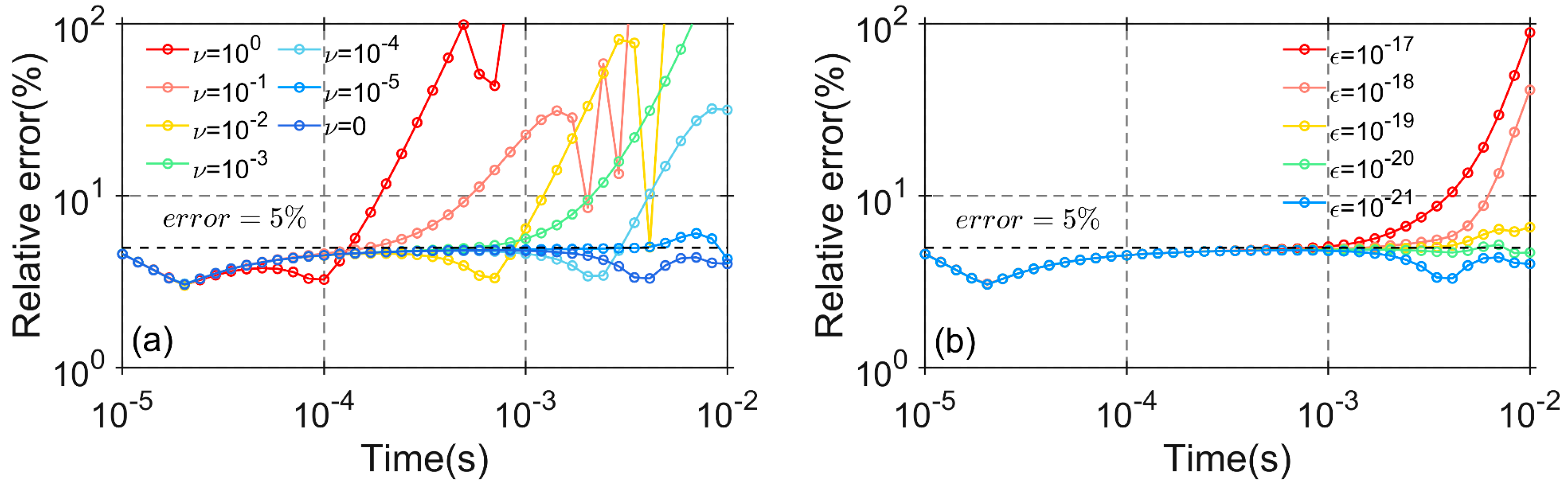
2.3. The Selection of the Initial Value and Tolerance for the PCG

This section describes the process for selecting the initial values for the iterative algorithm. The time range considered in this study is $\left[{10}^{-5},{10}^{-2}\right]$s. The conductivity of air and earth is ${\sigma }_{air}={10}^{-4} \mathrm{S}/\mathrm{m}$ and ${\sigma }_{earth}={10}^{-2} \mathrm{S}/\mathrm{m}$, respectively. The excitation device used in this study employs a grounded source, with a length of 100 m. According to Zhou et al., the optimal shift for this study is $\gamma =2.6\times {10}^{-7}$, and the Krylov subspace order is $m=320$ [26]. To ensure numerical accuracy, the tolerance $ϵ$ is chosen to be sufficiently small, with $ϵ={10}^{-21}$.

Figure 1a shows the relative error curves for different initial values, with the relative error varying significantly depending on the initial value. As seen in Figure 1a, the relative error decreases as the initial value decreases and eventually stabilizes. When the initial value is 100, the relative error changes dramatically, surpassing 100% around t = 1 ms. The relative error curves for initial values of ${10}^{-1}$ and ${10}^{-2}$ show similar characteristics to the curve with an initial value of ${10}^0$. However, the relative error trend becomes much gentler for initial values of ${10}^{-3}$ and ${10}^{-4}$, though it still does not meet the precision criteria for TEM forward simulations. When the initial value is further reduced, the relative error continues to decrease, and the curves become more stable.

Figure 1b shows the relative error curves for different tolerance values $ϵ$. In this study, a relative error of 5% is used to determine the tolerance $ϵ$ for the entire interval. As shown in Figure 1b, when the tolerance $ϵ$ is less than ${10}^{-20}$, the simulated TEM response does not meet the precision criteria. The relative error decreases and stabilizes as the tolerance decreases. When the tolerance is ${10}^{-20}$, the relative error curve nearly satisfies the criteria, although some relative errors still exceed 5% at certain times. To properly simulate the TEM response, the tolerance is set to ${10}^{-21}$, resulting in a minimum relative error of 3.1%, a maximum relative error of 4.8%, and an average relative error of 4.3%.

In summary, this paper sets the tolerance to $ϵ={10}^{-21}$ and the initial iteration value to 0. Furthermore, this study investigates the optimal tolerance and subspace order for different time periods in the following sections.

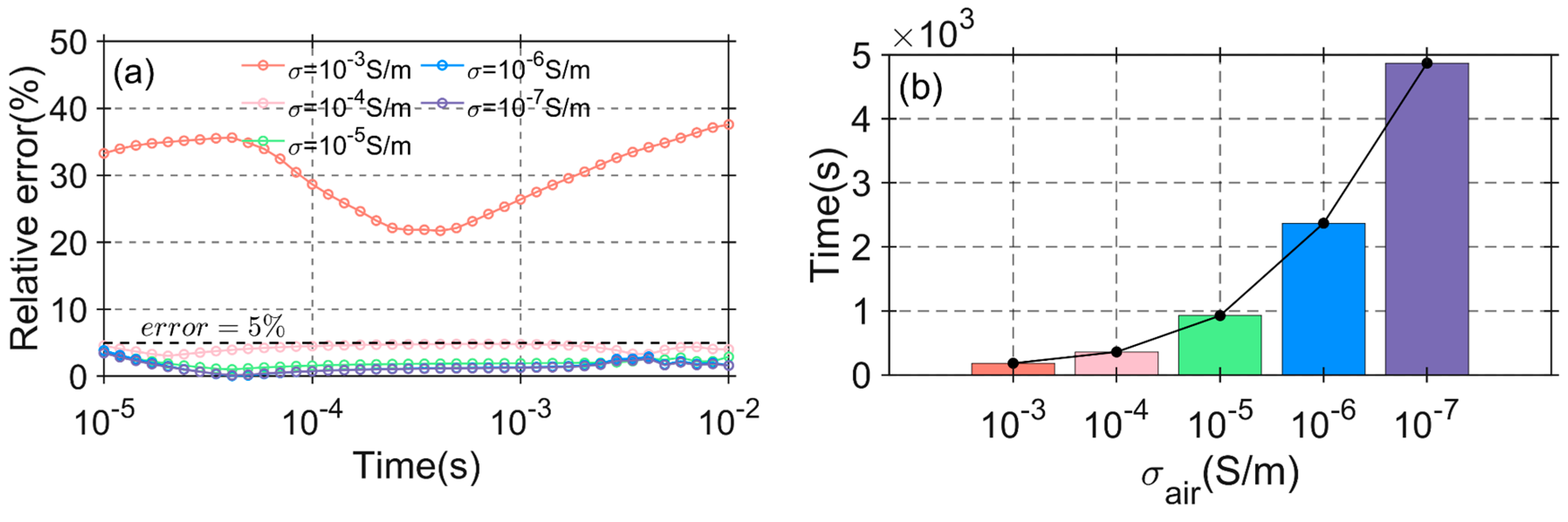
2.4. The Effect of Air Conductivity on the Algorithm

The conductivity of air cannot be considered infinitesimal when using numerical methods to simulate the TEM response, and a smaller value must be used to approximate the conductivity of air. Therefore, this section examines the effect of air conductivity on the computational process.

Figure 2a shows the relative error curves for different values of ${\sigma }_{air}$. As observed in Figure 2a, when ${\sigma }_{air}={10}^{-3} \mathrm{S}/\mathrm{m}$, the relative error is relatively high, with the minimum relative error exceeding 20%. When ${\sigma }_{air}={10}^{-4} \mathrm{S}/\mathrm{m}$, the relative error is significantly reduced, with the maximum relative error being less than 5%. Although the relative error decreases as air conductivity decreases, the precision of the TEM data does not improve substantially.

Figure 2b, on the other hand, shows the calculation times for different values of ${\sigma }_{air}$. As the air conductivity decreases, the computation time grows exponentially. The calculation times are 182 s, 359 s, 927 s, 2371 s, and 4873 s. Considering both numerical accuracy and computational efficiency, the air conductivity in this study is set to ${10}^{-4} \mathrm{S}/\mathrm{m}$.

Subsequently, this paper briefly analyzes why ${\sigma }_{air}$ has a significant effect on the calculation time. It is observed that the coefficient matrix is primarily influenced by ${\mu }_0$, $\sigma$, $\gamma$, and the grid size factor. As discussed earlier, ${\mu }_0$ and $\gamma$ are constants with values of $4\pi \times {10}^{-7}$ and $2.6\times {10}^{-7}$, respectively, indicating that the impact of ${\sigma }_{air}$ on the coefficient matrix is crucial.

Figure 3 shows the matrix condition number for different values of ${\sigma }_{air}$. It can be observed that when ${\sigma }_{air}$ is reduced by an order of magnitude, the condition number of the coefficient matrix decreases correspondingly. Comparing Figure 2b and Figure 3, it is evident that air conductivity affects the condition number of the coefficient matrix, which in turn adversely impacts the computation time. As shown in Figure 3, when ${\sigma }_{air}$ is reduced by an order of magnitude, the condition number of the coefficient matrix increases by an order of magnitude as well. Therefore, comparing Figure 2b and Figure 3 highlights that ${\sigma }_{air}$ significantly influences the condition number of the coefficient matrix, which greatly affects the computation time.

2.5. The Strategy of Time Division

Based on the above analysis, we set ${\sigma }_{air}={10}^{-4} \mathrm{S}/\mathrm{m}$, $ϵ={10}^{-21}$. In this study, the off-time is segmented into three periods: $\left[{10}^{-5},{10}^{-4}\right]\mathrm{s}$, $\left[{10}^{-4},{10}^{-3}\right]\mathrm{s}$, and $\left[{10}^{-3},{10}^{-2}\right]\mathrm{s}$. To more accurately simulate the later electromagnetic signals, the subspace order must be increased according to the principles of the Krylov subspace algorithm and the propagation behavior of the TEM diffusion field. In other words, the Krylov subspace method requires only a minimal subspace order to simulate the early electromagnetic signals.

Figure 4 shows the relative error for different Krylov subspace orders $m$. Figure 4a presents the relative error curve for the Krylov subspace order in the time interval $\left[{10}^{-5},{10}^{-4}\right]\mathrm{s}$. The accuracy of the calculation results does not meet the criteria when $m=50$, as shown in Figure 4a, with the maximum relative error exceeding 10%. However, as the Krylov subspace order is increased further, the relative error drops below 5%, and the relative error shows little change with further increases in $m$.

Figure 4b presents the relative error curve for the Krylov subspace order in the time interval $\left[{10}^{-4},{10}^{-3}\right]\mathrm{s}$. When $m=120$, as shown in Figure 4b, the precision of the computation results does not meet the criteria, with the maximum relative error exceeding 15%. Figure 4c shows the relative error curve for the Krylov subspace order in the time interval $\left[{10}^{-3},{10}^{-2}\right]\mathrm{s}$. The features of Figure 4c are similar to those of Figure 4a,b and therefore will not be discussed in detail.

The order of the subspace in different time intervals can be determined in this paper using the aforementioned analysis, as shown in

Table 1. The SAI-Krylov subspace order m in different time intervals.

Time Interval	$\left[{10}^{-5},{10}^{-4}\right]\mathbf{s}$	$\left[{10}^{-4},{10}^{-3}\right]\mathbf{s}$	$\left[{10}^{-3},{10}^{-2}\right]\mathbf{s}$
Subspace order m	$m_1=60$	$m_2=130$	$m_3=320$

.

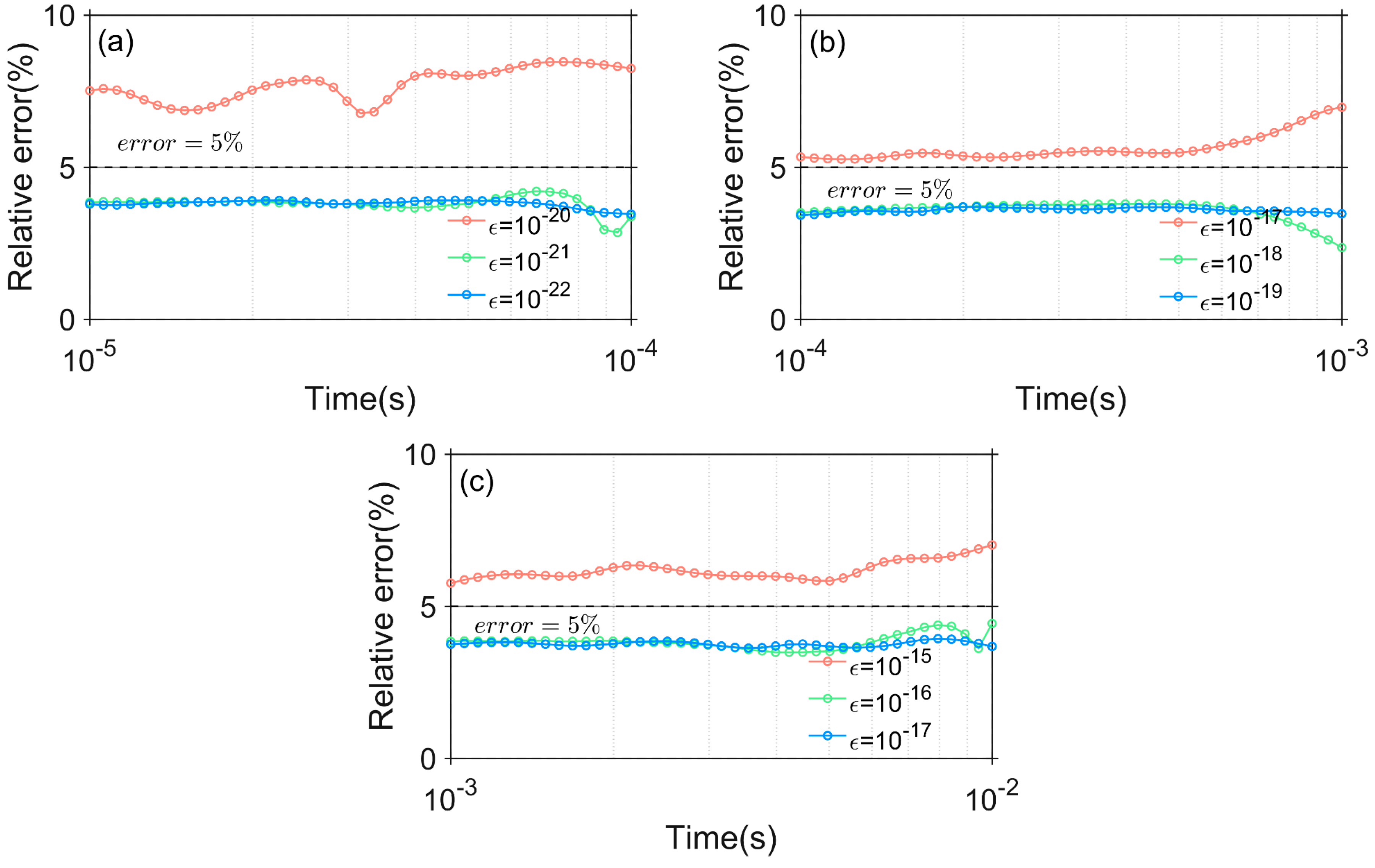
2.6. Optimal Tolerance ϵ and Relaxation Factor ω in Different Time Intervals

According to TEM propagation theory, the early diffusion field contains more high-frequency signals, while the later diffusion field is dominated by low-frequency components. As a result, the early time step is smaller, and the later time step is larger when the backward Euler method is used to solve the electromagnetic response. In constructing the orthogonal basis of the Krylov subspace, a time-step selection strategy is also employed in this study. The orthogonal basis of the Krylov subspace, as discussed earlier, is a dense matrix with $m$ columns, and ${\mathbf{V}}_{m1}$, ${\mathbf{V}}_{m2}$, and ${\mathbf{V}}_{m3}$ significantly influence the early, middle, and late forward responses, respectively. Consequently, different tolerances $ϵ$ can be applied when solving for ${\mathbf{V}}_{m1}$, ${\mathbf{V}}_{m2}$, and ${\mathbf{V}}_{m3}$ to optimize computational efficiency.

Figure 5 shows the relative error for different tolerance values $ϵ$. Figure 5a illustrates that when the time interval is $\left[{10}^{-5},{10}^{-4}\right]\mathrm{s}$ and $ϵ={10}^{-21}$, the relative error is relatively large, with the minimum relative error exceeding 5%. Figure 5b,c exhibit similar characteristics to Figure 5a. In the time interval $\left[{10}^{-4},{10}^{-3}\right]\mathrm{s}$, $ϵ={10}^{-18}$ satisfies the numerical accuracy requirements. Similarly, $ϵ={10}^{-16}$ meets the numerical accuracy criteria in the time interval $\left[{10}^{-3},{10}^{-2}\right]\mathrm{s}$.

To summarize, the tolerances $ϵ$ discussed in this paper are $ϵ={10}^{-21}$, $ϵ={10}^{-18}$, and $ϵ={10}^{-16}$ for the three separate time intervals. Following this, the paper will examine the effect of varying the relaxation factor across different time intervals on both the accuracy and computational time.

Table 2. The TEM results with different relaxation factors $\omega .$“√” means meet the calculation precision.

$\mathit{t}/\mathit{\omega }$	0.2	0.4	0.6	0.8	1.0	1.2	1.4	1.6	1.8
[10−5,10−4]s	√	√	√	√	√	√	√	√	√
[10−4,10−3]s	√	√	√	√	√	√	√	√	√
[10−3,10−2]s	√	√	√	√	√	√	√	√	√

shows the TEM results with different relaxation factors $\omega$. The relaxation factor $\omega$ has little impact on the accuracy of the TEM response, but has a noticeable effect on the convergence speed. When the relaxation factor $\omega =1$, the convergence speed is the fastest across all three time periods.

Figure 6 shows the relationship between the forward modeling computation time and the relaxation factor for different time intervals. It can be observed that when the relaxation factor is $\omega =1$, the computation efficiency is the highest. Therefore, based on the previous analysis, the optimal relaxation factor is $\omega =1$ for all three periods.

2.7. Comparison of Computational Performance

The TEM forward modeling parameters are as follows: air layer conductivity ${\sigma }_{air}={10}^{-4} \mathrm{S}/\mathrm{m}$, the tolerances are $ϵ={10}^{-21},{10}^{-18},{10}^{-16}$ for the three time intervals, and the SAI-Krylov subspace order is m = 320. This paper uses the time-segmented method, the SAI-Krylov subspace method [27], and the finite element method with an iterative method to simulate the TEM response, respectively.

For spatial discretization, all three methods use the same grid. The backward Euler strategy is employed for the iterative (FEM) method. To simulate the TEM response after turning off the current, 13 different iteration time steps, $∆t^k=2^{k-1}\times {10}^{-8}\mathrm{s}$, where $k=\mathrm{1,2},\dots ,13$, are used for the iterative method (FEM). During the computation process, 1300 linear equations need to be solved.

For the FEM direct method, when the number of unknowns is small, this method offers remarkably high computational efficiency. However, as the number of grids increases, memory usage grows exponentially. When the number of unknowns reaches 5,275,768, the method can no longer be used on the workstation due to memory limitations.

For the iterative method (FEM), the computation time has increased dramatically as the number of unknowns has grown. It is important to note that the time step used in this paper is not optimal. Using a suitable time step could further enhance the technique, but determining the optimal time step has always been a challenging task. The memory usage for the three iterative approaches is nearly the same, but the time-segmented SAI-Krylov subspace method offers the best computational efficiency.

The computation time and memory usage are shown in

Table 3. The comparison between the time-segmented SAI-Krylov solver and the other solvers, and “×” means beyond the calculation power of the computer.

Unknowns	Time-Segmented Method		Direct Method (FEM)		Iterative Method (FEM)
	Time	Memory	Times	Memory	Time	Memory
211,725	266 s	0.4 G	55 s	2.4 G	1808 s	0.4 G
689,789	997 s	0.8 G	241 s	8.1 G	2996 s	0.8 G
1,574,640	2730 s	1.5 G	851 s	21.6 G	17,384 s	1.5 G
3,160,300	6065 s	2.8 G	2255 s	51.5 G	37,166 s	2.8 G
5,275,768	10,815 s	4.9 G	×	×	62,987 s	4.9 G
8,550,025	16,286 s	7.5 G	×	×	104,414 s	7.5 G
12,642,086	27,783 s	11.2 G	×	×	151,442 s	11.2 G
17,690,940	39,679 s	16.2 G	×	×	217,680 s	16.2 G

. These three techniques can yield TEM responses with the same precision (less than 5%), but there are significant differences in calculation time and memory usage.

3. Numerical Experiments

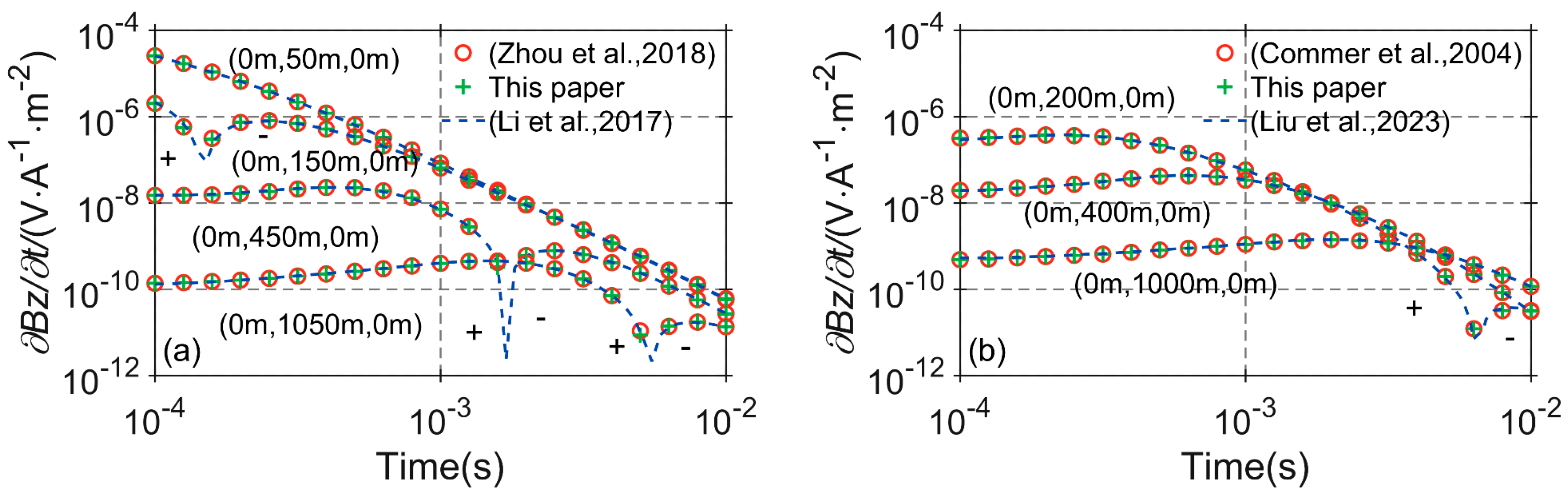
The above content introduces the large-scale forward modeling method and its parameter optimization strategy. Next, this paper first validates the accuracy of the proposed method using a layered model and a three-dimensional vertical contact band model. Then, two complex geological models are used to study the propagation characteristics of the electromagnetic field in the xoz and xoy planes, respectively.

3.1. Layer Model

The layered model is shown in Figure 7. It consists of a conductive layer with a burial depth of 100 m, a thickness of 20 m, and a conductivity of $10 \mathsf{\Omega }·\mathrm{m}$, situated in a half-space with a conductivity of $200 \mathsf{\Omega }·\mathrm{m}$. A grounded wire is used as the transmitter, with a length of 100 m. The coordinates of the two endpoints are (−50 m, −50 m, 0 m) and (−50 m, −50 m, 0 m), and the receiver is located at (0 m, 0 m, 0 m). The time range for the forward simulation is from 10⁻⁵ s to 10⁻² s, with a total of 31 time gates. The minimum grid size is 10 m, resulting in 238,964 unknowns and a computation time of 352 s.

Figure 8 presents the computational results for this model, where Figure 8a and Figure 8b represent the horizontal component of the electric field and the vertical component of the induced electromotive force, respectively. Figure 8c shows the relative error compared to the one-dimensional results. The relative errors for both the horizontal component of the electric field and the vertical component of the induced electromotive force are less than 5%, validating the effectiveness and accuracy of the numerical simulation method proposed in this paper.

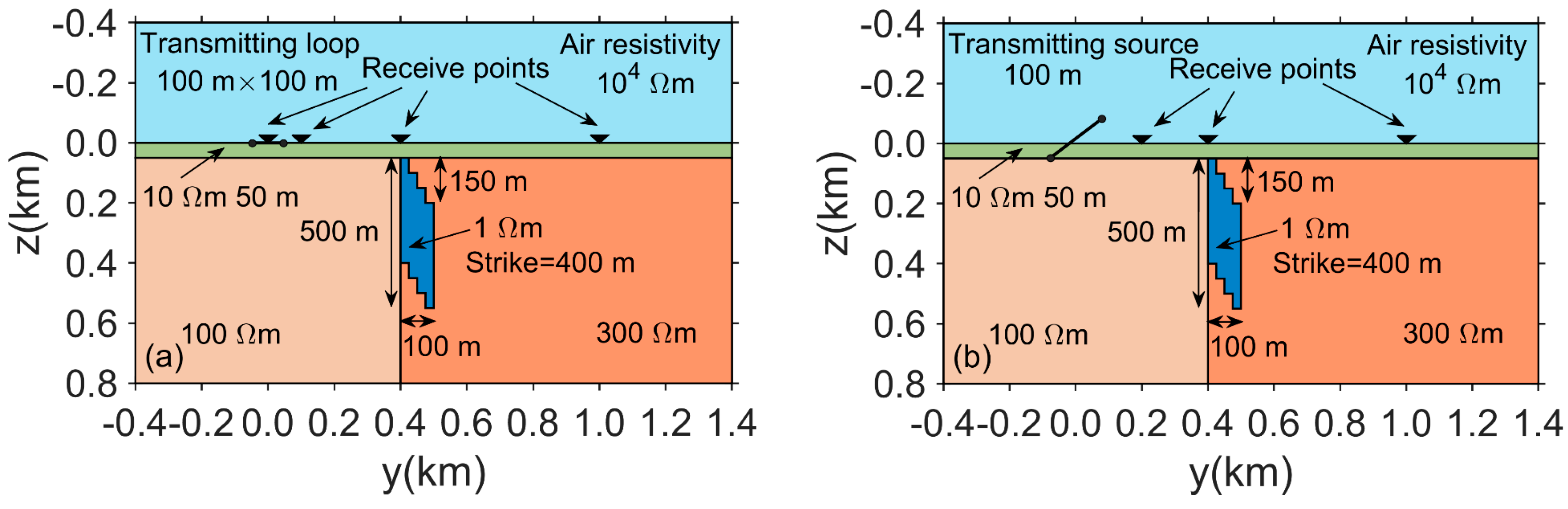
3.2. Three-Dimensional Vertical Contact Model

The three-dimensional vertical contact band model is used to further validate the forward modeling method proposed in this paper, as shown in the schematic diagram in Figure 9. The resistivity of air is set to ${\rho }_{air}={10}^4 \mathsf{\Omega }·\mathrm{m}$, and a low-resistivity cover layer of 50 m thickness is placed on the surface, with a resistivity of $10 \mathsf{\Omega }·\mathrm{m}$. Below the cover layer, the resistivity of the strata on the left side is $100 \mathsf{\Omega }·\mathrm{m}$, and the resistivity of the strata on the right side is $300 \mathsf{\Omega }·\mathrm{m}$. A step-shaped geological body with a resistivity of $1 \mathsf{\Omega }·\mathrm{m}$ is located in the middle of the strata. This geological body has a length of 400 m along the x-axis, a width of 100 m along the y-axis, and a thickness of 500 m along the z-axis. The accuracy of the method is tested using both a loop source and a grounded wire source. The loop source is placed on the surface, with a side length of 100 m, and its center is located at (0 m, 50 m, 0 m). The four receiver points are positioned along the y-axis at 50 m, 150 m, 450 m, and 1050 m. The grounded wire source is placed along the x-axis, with its endpoints at (−50 m, 0 m, 0 m) and (50 m, 0 m, 0 m), and three receiver points are positioned along the y-axis at 200 m, 400 m, and 1000 m. The minimum grid size is 5 m, resulting in 1,357,187 unknowns and a computation time of 2171 s.

Figure 10a and Figure 10b show the induced electromotive force (z-component) curves at different receiver points for the loop source and grounded wire source, respectively. In Figure 10a, the electromagnetic signal at the receiver point (0 m, 50 m, 0 m) decays normally. However, for the receiver points (0 m, 150 m, 0 m), (0 m, 450 m, 0 m), and (0 m, 1050 m, 0 m), which are located outside the loop source, the corresponding decay curves exhibit a turning point, with the sign of the electromagnetic field reversing before and after the turning point. In Figure 10b, as the offset distance increases and the geological anomaly’s influence grows, the early induced electromotive force (z-component) does not decay significantly in the double-logarithmic coordinate system. In fact, the electromagnetic signal slightly increases before it gradually decays. Additionally, due to the impact of the low-resistivity anomaly, the electromagnetic field at the receiver point (0 m, 1000 m, 0 m) undergoes a reversal in sign. The three-dimensional vertical contact band model further validates the effectiveness of the proposed method.

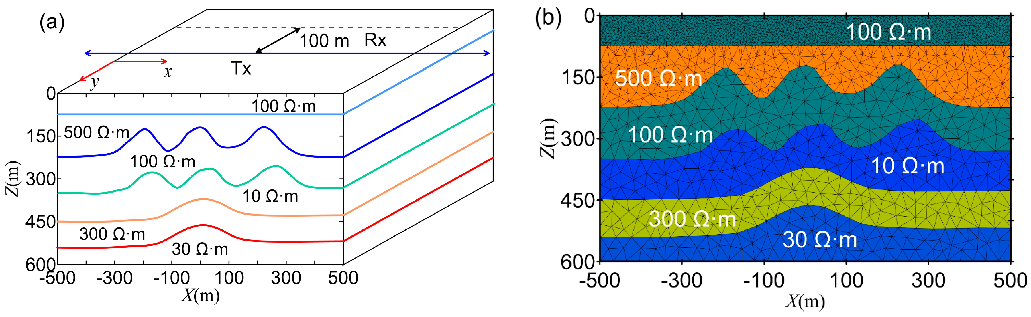
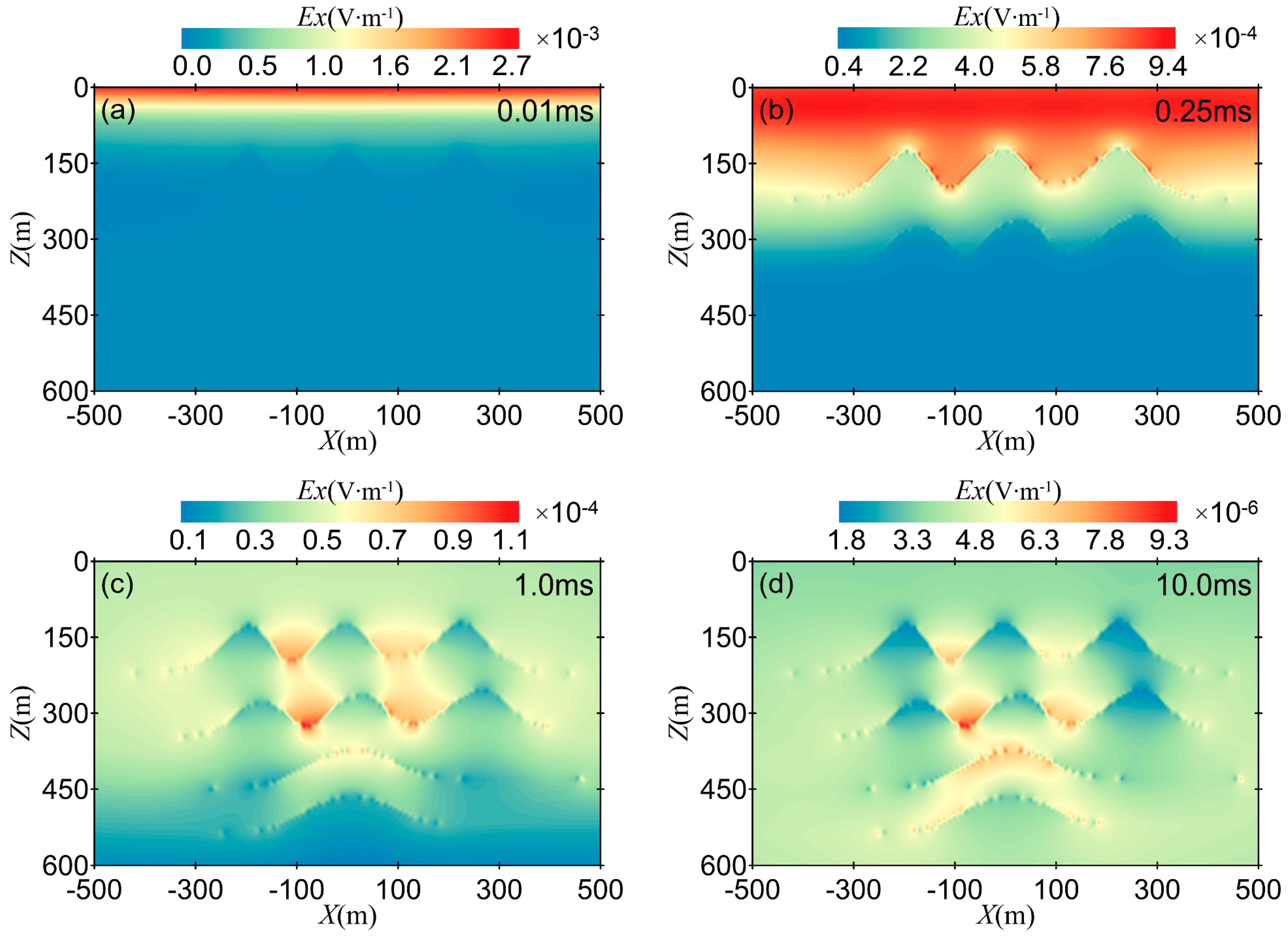
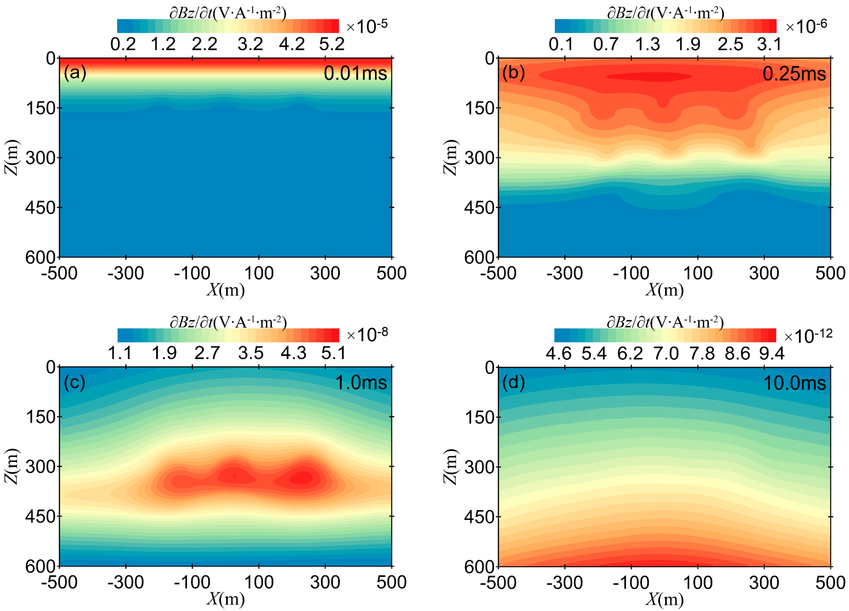
3.3. Large-Scale Undulating Stratigraphy Model

This paper constructs a two-dimensional large-scale model with five layers of complex interfaces. Figure 11 shows the resistivity distribution of the formations across the complex interface, which spans from −500 m to 500 m along the x-axis. A long wire source is used to transmit and receive the TEM response ${\mathit{E}}_x$ and $\partial {\mathit{B}}_z/\partial t$. The long wire source has a length of 2 km, with its coordinates at (−1000 m, 100 m, 0 m) and (1000 m, 100 m, 0 m), and an emission current of 1 A. The receiving survey line, with a length of 1 km, is positioned along the x-axis, with endpoint coordinates at (−500 m, 0 m, 0 m) and (500 m, 0 m, 0 m). To achieve high-precision forward responses and properly model topographic fluctuations, the minimum mesh length used in this study is 5 m, and the grid division diagram is shown in Figure 11. The minimum grid size is 10 m, with the total number of unknowns reaching 7.4 million and a computation time of 14,984 s. On the other hand, the memory usage of this method is only 6.3 GB.

Figure 12 shows cross-sectional views of the electric field ${\mathit{E}}_x$ at 0.01 ms, 0.25 ms, 1 ms, and 10 ms. At t = 0.01 ms, the electric field ${\mathit{E}}_x$ is mostly concentrated near the surface, and the interface topography of the first and second layers can be vaguely observed in Figure 12a. At t = 0.25 ms, the electric field ${\mathit{E}}_x$ gradually diffuses downwards, and the formation geometry of the second and third layers becomes clearer, although the deep-layer formation information is not fully reflected. As time progresses, at t = 1 ms, the geometry of the undulating formation aligns well with the contour distribution of the electric field ${\mathit{E}}_x$. The distribution of ${\mathit{E}}_x$ at t = 10 ms is similar to that at t = 1 ms, but the extreme value of the electric field ${\mathit{E}}_x$ decreases and diffuses deeper into the formation.

Figure 13 shows cross-sectional views of the induced electromotive force $\partial {\mathit{B}}_z/\partial t$ at 0.01 ms, 0.25 ms, 1 ms, and 10 ms, respectively. Figure 13a is similar to Figure 12a, as both effectively reflect the shallow horizontal stratigraphic interfaces and show a slight response to the first undulating interface. However, the electromagnetic anomaly in Figure 13a is weaker than that in Figure 12a. Figure 13b,c capture the undulating strata and the underlying stratigraphic uplift, but compared to Figure 12b,c, the electromagnetic field anomalies show lower consistency with the undulating stratigraphic morphology. When the diffusion time reaches t = 10 ms, the electromagnetic anomaly in the shallow strata of Figure 13d disappears, making it difficult to accurately capture the structural morphology of the deeper strata.

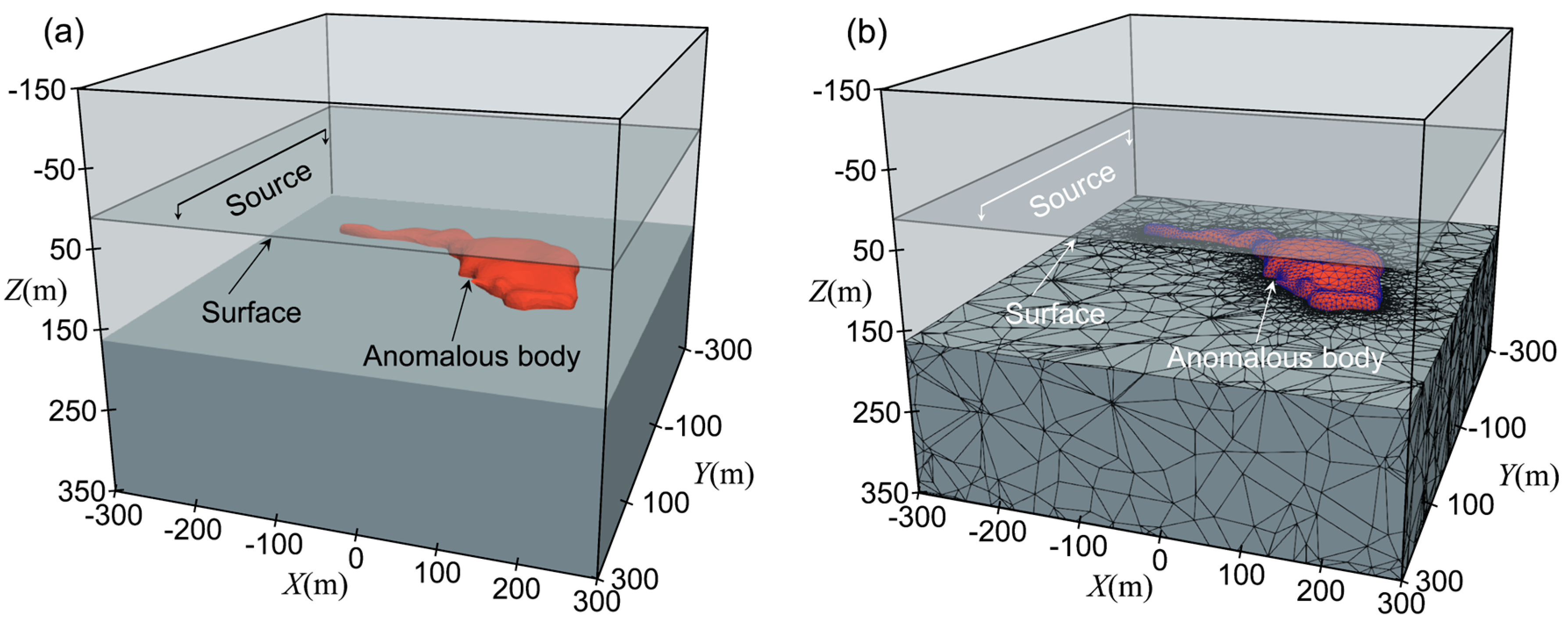
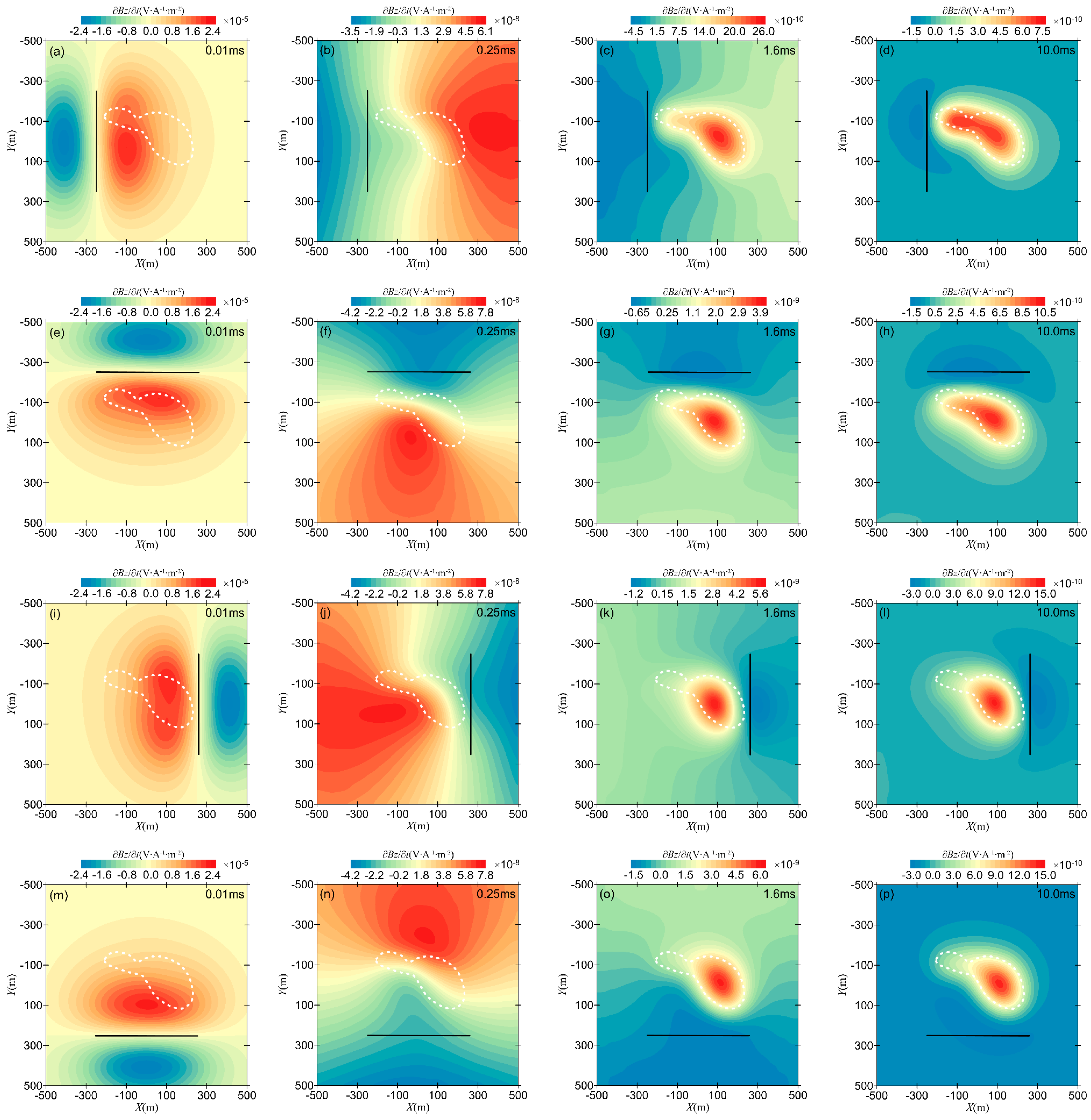
3.4. Large-Scale Sulfide Model

To further validate the effectiveness and feasibility of the proposed method for large-scale forward modeling, as shown in Figure 14. Figure 14a presents the model schematic diagram, and Figure 14b shows the tetrahedral mesh division. This model is derived from a sulfide deposit in Labrador, Canada, which has a shape resembling a sprout-like block of sulfide ore. Based on related drilling data, the length of the ore body in the x-direction is approximately 400 m, its width in the y-direction is about 300 m, and its thickness in the z-direction is about 115 m. In this study, a grounded wire is used as the transmitter with a length of 500 m and a current of 1 A. Both the transmitter and the receiver are located on the surface (terrain effects are not considered), and the receiving area extends from −500 m to 500 m in both the x- and y-directions. The uniform half-space resistivity is set to $100 \mathsf{\Omega }·\mathrm{m}$, and the resistivity of the sulfide ore body is set to $0.01 \mathsf{\Omega }·\mathrm{m}$. The minimum grid size is 10 m, with the total number of unknowns reaching 8.7 million and a computation time of 17,875 s. On the other hand, the memory usage of this method is only 7.6 GB.

Figure 15 shows the contour maps of the horizontal electric field component in the xoy plane for different transmitter positions. Figure 15a–d correspond to transmitter coordinates at (−250 m, −250 m, 0 m) and (−250 m, 250 m, 0 m); Figure 15e–h correspond to transmitter coordinates at (−250 m, −250 m, 0 m) and (250 m, −250 m, 0 m); Figure 15i–l correspond to transmitter coordinates at (250 m, −250 m, 0 m) and (250 m, 250 m, 0 m); and Figure 15m–p correspond to transmitter coordinates at (−250 m, 250 m, 0 m) and (250 m, 250 m, 0 m). Each transmitter’s anomaly contour includes four time steps: 0.01 ms, 0.25 ms, 1.6 ms, and 10.0 ms.

From Figure 15, it can be seen that at t = 0.01 ms, the electric field is mainly concentrated in the shallow strata and spreads in an elliptical shape from the transmitter to the surrounding area. At t = 0.25 ms, due to the influence of the low-resistivity body, the electric field amplitude is relatively higher on both sides of the anomaly. As time progresses, the contour lines of the horizontal electric field component gradually align with the shape of the anomaly, and the electric field strength decreases. The white dotted line in the Figure 15 is the contour of the anomalous body in the xoy plane.

Figure 16 shows the contour maps of the induced electromotive force (z-component) in the xoy plane for different transmitter positions, with the transmitter coordinates and observation times held constant. From Figure 16, it can be observed that for transmitters at different positions, when the current is turned off at t = 0.01 ms, the electromagnetic anomaly is approximately symmetrically distributed on both sides of the transmitter. At t = 0.25 ms, due to the influence of the low-resistivity body, the contour lines of the induced electromotive force show significant distortion at the center of the anomaly. At t = 1.6 ms, the contour lines for different transmitter positions align relatively well with the outer boundary of the anomaly, although the degree of alignment varies. As time progresses further, the contour lines of the induced electromotive force gradually concentrate within the anomaly body, and the amplitude decreases. The white dotted line in the Figure 16 is the contour of the anomalous body in the xoy plane.

4. Conclusions

In this study, we have developed an algorithm for simulating large-scale TEM responses based on the finite element and time-segmented SAI-Krylov subspace methods. This approach enables efficient simulation of large-scale TEM responses within an acceptable time frame while using less memory. The optimization parameters of the method, including the initial value, air conductivity ${\sigma }_{air}$, tolerance $ϵ$, relaxation factor $\omega$, and subspace order across different time intervals, were discussed in detail. The numerical simulation results show that the TEM response simulated by the proposed method is both accurate and reliable, laying the foundation for future research in large-scale inversion and TEM interpretation.

While the proposed method achieves efficient large-scale 3D TEM forward modeling, there are still some limitations. Firstly, the selection of parameters in the algorithm is based on layered medium models, which may not be directly applicable to arbitrary 3D geological models. To address this limitation, future research will focus on optimizing parameter selection for random media. Secondly, the current method can benefit from the development of an adaptive SAI-Krylov subspace iterative algorithm, which could further improve computational efficiency. These aspects will be investigated in future studies to enhance the applicability and performance of the proposed method in more complex geological scenarios.

References

1. Vallee, M.A.; Smith, R.S.; Keating, P. Metalliferous mining geophysics—State of the art after a decade in the new millennium. Geophysics 2011, 76, W31–W50. [Google Scholar] [CrossRef]
2. Fournier, D.; Kang, S.; McMillan, M.S.; Oldenburg, D.W. Inversion of airborne geophysics over the DO-27/DO-18 kimberlites-Part 2: Electromagnetics. Interpretation 2017, 5, T313–T325. [Google Scholar] [CrossRef]
3. Di, Q.Y.; Xue, G.Q.; Yin, C.C.; Li, X. New methods of controlled-source electromagnetic detection in China. Sci. China Earth Sci. 2020, 50, 1219–1227. [Google Scholar] [CrossRef]
4. Lu, K.L.; Fan, Y.N.; Li, X.; Zhou, J.M.; Fan, K.R. Transient electromagnetic pseudo wavefield imaging based on the sweep-time preconditioned precise integration algorithm. J. Appl. Geophys. 2023, 209, 104937. [Google Scholar] [CrossRef]
5. Jiang, Z.H.; Liu, L.B.; Liu, S.C.; Yue, J.H. Surface-to-Underground Transient Electromagnetic Detection of Water-Bearing Goaves. IEEE Trans. Geosci. Remote Sens. 2019, 57, 5303–5318. [Google Scholar] [CrossRef]
6. Xue, G.Q.; Zhang, L.B.; Zhou, N.N.; Chen, W.Y. Developments measurements of TEM sounding in China. Geol. J. 2020, 55, 1636–1643. [Google Scholar] [CrossRef]
7. Lu, K.L.; Li, X.; Fan, Y.N.; Zhou, J.M.; Qi, Z.P.; Li, W.H.; Li, H. The application of multi-grounded source transient electromagnetic method in the detections of coal seam goafs in Gansu Province, China. J. Geophys. Eng. 2021, 18, 515–528. [Google Scholar] [CrossRef]
8. Li, S.C.; Sun, H.F.; Lu, X.S.; Li, X. Three-dimensional modeling of transient electromagnetic responses of water-bearing structures in front of a tunnel face. J. Environ. Eng. Geophys. 2014, 19, 13–32. [Google Scholar] [CrossRef]
9. Liu, B.; Fan, K.R.; Nie, L.C.; Li, X.; Liu, F.S.; Li, L.M.; Wang, J.S.; Sun, H.F.; Chen, L. Mapping water-abundant zones using transient electromagnetic and seismic methods when tunneling through fractured granite in the Qinling Mountains, China. Geophysics 2020, 85, B147–B159. [Google Scholar] [CrossRef]
10. Auken, E.; Foged, N.; Larsen, J.J.; Lassen, K.V.T.; Maurya, P.K.; Dath, S.M.; Eiskjær, T.T. tTEM-towed transient electromagnetic system for Detailed 3D Imaging of the top 70 m of the subsurface. Geophysics 2019, 84, E13–E22. [Google Scholar] [CrossRef]
11. Gottschalk, I.; Knight, R.; Asch, T.; Abraham, J.; Cannia, J. Using an airborne electromagnetic method to map saltwater intrusion in the northern Salinas Valley, California. Geophysics 2020, 85, B119–B131. [Google Scholar] [CrossRef]
12. Yin, C.C.; Liu, Y.H.; Xiong, B. Status and prospect of 3D inversions in EM geophysics. Sci. China Earth Sci. 2020, 63, 452–455. [Google Scholar] [CrossRef]
13. Wang, T.; Hohmann, G.W. A finite-difference, time-domain solution for three-dimensional electromagnetic modeling. Geophysics 1993, 58, 797–809. [Google Scholar] [CrossRef]
14. Commer, M.; Newman, G. A parallel finite-difference approach for 3D transient electromagnetic modeling with galvanic sources. Geophysics 2004, 69, 1192–1202. [Google Scholar] [CrossRef]
15. Sun, H.F.; Li, X.; Li, S.C.; Qi, Z.P.; Wang, Y.P.; Su, M.X.; Xue, Y.G.; Liu, B. Three-dimensional FDTD modeling of TEM excited by a loop source considering ramp time. Chin. J. Geophys. 2013, 56, 1049–1064. [Google Scholar]
16. Ji, Y.J.; Wu, Y.; Guan, S.; Zhao, X. 3D numerical modeling of induced-polarization electromagnetic response based on the finite-difference time-domain method. Geophysics 2018, 83, E385–E398. [Google Scholar] [CrossRef]
17. Um, E.S.; Harris, J.M.; Alumbaugh, D.L. An iterative finite element time-domain method for simulating three-dimensional electromagnetic diffusion in earth. Geophys. J. Int. 2012, 190, 871–886. [Google Scholar] [CrossRef]
18. Oldenburg, D.W.; Haber, E.; Shekhtman, R. Three dimensional inversion of multisource time domain electromagnetic data. Geophysics 2013, 78, E47–E57. [Google Scholar] [CrossRef]
19. Fu, H.; Wang, Y.; Um, E.S.; Fang, J.; Wei, T.; Huang, X.; Yang, G. A parallel finite-element time-domain method for transient electromagnetic simulation. Geophysics 2015, 80, E213–E224. [Google Scholar] [CrossRef]
20. Yin, C.C.; Qi, Y.F.; Liu, Y.H. 3D time-domain airborne EM modeling for an arbitrarily anisotropic earth. J. Appl. Geophys. 2016, 131, 163–178. [Google Scholar] [CrossRef]
21. Qi, Y.F.; Yin, C.C.; Liu, Y.H.; Cai, J. 3D time-domain airborne EM full-wave forward modeling based on instantaneous current pulse. Chin. J. Geophys. 2017, 60, 369–382. [Google Scholar]
22. Druskin, V.; Knizhnerman, L. Spectral approach to solving three-dimensional Maxwell’s diffusion equations in the time and frequency domains. Radio Sci. 1994, 29, 937–953. [Google Scholar] [CrossRef]
23. Zaslavsky, M.; Druskin, V.; Knizhnerman, L. Solution of 3D time-domain electromagnetic problems using optimal subspace projection. Geophysics 2011, 76, F339–F351. [Google Scholar] [CrossRef]
24. Sommer, M.; Hölz, S.; Moorkamp, M.; Swidinsky, A.; Heincke, B.; Scholl, C.; Jegen, M. GPU parallelization of a three dimensional marine CSEM code. Comput. Geosci. 2013, 58, 91–99. [Google Scholar] [CrossRef]
25. Börner, R.U.; Ernst, O.G.; Güttel, S. Three-dimensional transient electromagnetic modelling using rational Krylov methods. Geophys. J. Int. 2015, 202, 2025–2043. [Google Scholar] [CrossRef]
26. Zhou, J.M.; Liu, W.T.; Li, X.; Qi, Z.P. 3D transient electromagnetic modeling using a shift-and-invert Krylov subspace method. J. Geophys. Eng. 2018, 15, 1341–1349. [Google Scholar] [CrossRef]
27. Lu, K.L.; Fan, Y.N.; Zhou, J.M.; Li, X.; Fan, K.R. 3D anisotropic TEM modeling with loop source using model reduction method. J. Geophys. Eng. 2022, 19, 403–417. [Google Scholar] [CrossRef]
28. Li, J.H.; Farquharson, C.G.; Hu, X.Y. 3D vector finite-element electromagnetic forward modeling for large loop sources using a total-field algorithm and unstructured tetrahedral grids. Geophysics 2017, 82, E1–E16. [Google Scholar] [CrossRef]
29. Haber, E.; Oldenburg, D.W.; Shekhtman, R. Inversion of time domain three-dimensional electromagnetic data. Geophys. J. Int. 2007, 171, 550–564. [Google Scholar] [CrossRef]
30. Hochbruck, M.; Lubich, C. On Krylov subspace approximations to the matrix exponential operator. SIAM J. Numer. Anal. 1997, 34, 1911–1925. [Google Scholar] [CrossRef]
31. Van, D.E.J.; Hochbruck, M. Preconditioning Lanczos approximations to the matrix exponential. SIAM J. Sci. Comput. 2006, 27, 1438–1457. [Google Scholar]
32. Liu, W.T.; Farquharson, C.G.; Zhou, J.M.; Li, X. A rational Krylov subspace method for 3D modeling of grounded electrical source airborne time-domain electromagnetic data. J. Geophys. Eng. 2019, 16, 451–462. [Google Scholar] [CrossRef]
33. Li, J.H.; Zhu, Z.Q.; Liu, S.C.; Zeng, S.H. 3D numerical simulation for the transient electromagnetic field excited by the central loop based on the vector finite-element method. J. Geophys. Eng. 2011, 8, 560–567. [Google Scholar] [CrossRef]
34. Altaf, S.; Sani, F.; Akram, S. Comparative study of some iterative methods for nonlinear equations from a dynamical point of view. J. Mt. Area Res. 2024, 9, 46–53. [Google Scholar]
35. Wu, X.P.; Xu, G.M. Study on 3-D resistivity inversion using conjugate gradient method. Chin. J. Geophys. 2000, 43, 450–458. [Google Scholar]
36. Wu, X.P.; Wang, T.T. A 3-D finite-element resistivity forward modeling using conjugate gradient algorithm. Chin. J. Geophys. 2003, 46, 428–432. [Google Scholar]
37. Peng, R.H.; Hu, X.Y.; Han, B. 3D inversion of frequency-domain CSEM data based on Gauss-Newton optimization. Chin. J. Geophys. 2016, 59, 3470–3481. [Google Scholar]
38. Kazemi, N. Shot-record extended model domain preconditioners for least-squares migration. Geophysics 2019, 84, S285–S299. [Google Scholar] [CrossRef]
39. Ma, G.Q.; Zhou, B.; Riahi, M.K.; Zemerly, J.; Xu, L. On cost-efficient parallel iterative solvers for 3D frequency-domain seismic multisource viscoelastic anisotropic wave modeling. Geophysics 2024, 89, T151–T162. [Google Scholar] [CrossRef]
40. Fang, Z.L.; Wang, H. GPU accelerated sparse curvelet-constrained wavefield reconstruction inversion with source estimation: Application to Chevron Benchmark 2014 blind test data set. Geophysics 2024, 89, R443–R455. [Google Scholar] [CrossRef]
41. Li, J.H.; Wang, Y. Effects of base frequency, duty cycle, and waveform repetition on transient electromagnetic responses: Insights from models of a deep-buried conductor. Geophysics 2024, 89, E165–E176. [Google Scholar] [CrossRef]
42. Gao, R.Y.; Yin, C.C.; Liang, H.; Liu, Y.H.; Wang, L.Y.; Su, Y.; Xiong, B. Three-dimensional simulation and characterization of airborne transient electromagnetic response in rough media. Geophysics 2024, 89, E61–E71. [Google Scholar] [CrossRef]
43. Lu, K.L.; Yue, J.H.; Fan, Y.N.; Li, X.; Zhou, J.M.; Qi, Y.F. Three-dimensional transient electromagnetic large-scale forward modeling based on unstructured tetrahedral mesh. Chin. J. Geophys. 2025, 68, 327–341. [Google Scholar]
44. Lu, K.L.; Yue, J.H.; Zhou, J.M.; Fan, Y.N.; Fan, K.R.; Li, H.; Li, X. Quadrature-based restarted Arnoldi method for fast 3-D TEM forward modeling of large-scale models. IEEE Geosci. Remote Sens. 2025, 68, 327–341. [Google Scholar] [CrossRef]
45. Saad, Y. Iterative Methods for Sparse Linear Systems; SIAM: Philadelphia, PA, USA, 2003. [Google Scholar]
46. Higham, N.J. The scaling and squaring method for the matrix exponential revisited. SIAM J. Matrix Anal. Appl. 2005, 26, 1179–1193. [Google Scholar] [CrossRef]
47. Liu, S.B.; Sun, H.F.; Li, W.H.; Wang, Z.; Yang, Y. 3D transient electromagnetics forward modeling using BEDS-FDTD and its stability verification. Chin. J. Geophys. 2023, 66, 841–853. [Google Scholar]
Figure 1. The influence of initial value and tolerance on the computational results: (a) relative error corresponding to different initial values; (b) relative error corresponding to different tolerances.
Applsci 15 05359 g001
Figure 2. The influence of air conductivity on the computational results: (a) relative error curves of different σ a i r ; (b) calculation time of different σ a i r .
Applsci 15 05359 g002
Figure 3. The matrix condition number of different σ a i r .
Applsci 15 05359 g003
Figure 4. The relative error with different SAI-Krylov subspace order m: (a) 10 5 , 10 4 s ; (b) 10 4 , 10 3 s ; (c) 10 3 , 10 2 s .
Applsci 15 05359 g004
Figure 5. The relative error with different tolerances ϵ : (a) 10 5 , 10 4 s ; (b) 10 4 , 10 3 s ; (c) 10 3 , 10 2 s .
Applsci 15 05359 g005
Figure 6. The calculation time with different relaxation factors ω : (a) 10 5 , 10 4 s ; (b) 10 4 , 10 3 s ; (c) 10 3 , 10 2 s .
Applsci 15 05359 g006
Figure 7. Layer model.
Applsci 15 05359 g007
Figure 8. The computational results of the layered model: (a) E x data; (b) B z / t data; (c) relative error.
Applsci 15 05359 g008
Figure 9. Three-dimensional complex model with a vertical contact zone: (a) loop source device; (b) grounded source device.
Applsci 15 05359 g009
Figure 10. The numerical results of 3D vertical contact zone: (a) loop source device [16,28]; (b) grounded source device [14,47].
Applsci 15 05359 g010
Figure 11. Two-dimensional undulating stratigraphy model: (a) model schematic diagram; (b) grid division diagram.
Applsci 15 05359 g011
Figure 12. Cross-sectional views of the electric field E x : (a) 0.01 ms; (b) 0.25 ms; (c) 1 ms; (d) 10 ms.
Applsci 15 05359 g012
Figure 13. Cross-sectional views of the electric field B z / t : (a) 0.01 ms; (b) 0.25 ms; (c) 1 ms; (d) 10 ms.
Applsci 15 05359 g013
Figure 14. Three-dimensional large-scale sulfide model: (a) model schematic diagram; (b) grid division diagram.
Applsci 15 05359 g014
Figure 15. Contour map of the horizontal electric field component in the xoy plane for different transmitter positions: (ad) source coordinates are (−250 m, −250 m, 0 m) and (−250 m, 250 m, 0 m); (eh) source coordinates are (−250 m, −250 m, 0 m) and (250 m, −250 m, 0 m); (il) source coordinates are (250 m, −250 m, 0 m) and (250 m, 250 m, 0 m); (mp) source coordinates are (−250 m, 250 m, 0 m) and (250 m, 250 m, 0 m).
Applsci 15 05359 g015
Figure 16. Contour map of the B z / t in the xoy plane for different transmitter positions: (ad) source coordinates are (−250 m, −250 m, 0 m) and (−250 m, 250 m, 0 m); (eh) source coordinates are (−250 m, −250 m, 0 m) and (250 m, −250 m, 0 m); (il) source coordinates are (250 m, −250 m, 0 m) and (250 m, 250 m, 0 m); (mp) source coordinates are (−250 m, 250 m, 0 m) and (250 m, 250 m, 0 m).
Applsci 15 05359 g016