An Integrated Capacity Allocation and Dynamic Pricing Model Designed for Air Cargo Transportation

Featured Application

An integrated capacity allocation and dynamic pricing model designed for air cargo transportation.

Abstract

Air cargo plays a pivotal role in the global economy by facilitating international trade. Air cargo companies must meticulously plan and price their limited capacity efficiently to gain a competitive advantage and enhance their profitability. To mitigate the risk of empty aircraft, companies can sell capacity through prior agreements or offer capacity for free sales to generate additional revenue. The intricate nature of the air cargo industry, coupled with the numerous variables that influence pricing within this sector, renders the dynamic determination of prices a complex and arduous undertaking. This study aims to dynamically determine the price for the free sales capacity. The proposed model addresses three critical issues in air cargo revenue management: capacity allocation, demand forecasting, and dynamic pricing. An integrated structure has been developed in which these three distinct issues are interconnected. In this study, CVaR and ANN models are used for capacity allocation, regression, and time series, and ANN models are used for demand forecasting, while the SARSA algorithm, one of the reinforcement learning algorithms, is used for dynamic pricing. The model is implemented using data from a prominent air cargo company, and the results are interpreted, and recommendations are made for future research.

1. Introduction and Background

Since the 20th century, air cargo transportation has played an important role in world trade. It is differentiated from other modes of transportation due to the speed, efficiency, and access to remote locations it provides. Thanks to these features, air cargo transportation becomes quite suitable for the transportation of products such as temperature-sensitive and time-sensitive goods, perishable goods, high-value goods, live animal transportation, and high-tech products [1].

In the present era, air cargo plays an indispensable role in economic growth and is a principal facilitator of international trade. The global reach of businesses is enhanced by air cargo. The demand for air cargo is driven by economic growth and the process of globalization. For air cargo companies to continue their activities, it is essential for them to manage their existing resources effectively. At this juncture, accurately managing the capacity of air cargo companies will positively impact their profitability.

Prior to the mid-1980s, studies in air cargo transportation primarily focused on descriptive analyses of the sector, operational processes, and developments. Subsequently, there was a notable shift towards the application of quantitative decision-making techniques in numerous studies on operational processes within the air cargo transportation domain. In recent years, there has been a notable increase in the number of studies on air cargo transportation [2].

The objective of air cargo companies is to maximize aircraft utilization and revenue by offering their available capacity at an optimal price and quantity. In the context of the air cargo sector, capacity can be pre-sold through the use of allocation agreements or retained for future sale in anticipation of demand (free sale). It is therefore crucial to ascertain the extent to which total capacity is committed to allocation agreements in order to guarantee optimal capacity utilization. Once the manner in which capacity will be allocated has been established, the pricing of capacity allocated for free sale represents a crucial issue with significant implications for revenue and profitability for air cargo companies.

A variety of pricing strategies are put into practice in business contexts. These include cost-based pricing, value-based pricing, break-even pricing, dynamic pricing, competitive pricing, daily low pricing, target return pricing, and margin pricing [3].

Dynamic pricing is a highly flexible approach that enables an online platform to adjust the price of a product offered for sale in real time based on market conditions. The selection of an optimal pricing model serves as a pivotal strategic decision for firms. As a result of the Airline Deregulation Act of 1978 in the US and the Third Deregulation Act of 1977 in Europe, competition in the airline and air cargo industry has accelerated, and firms have been able to regulate their prices. Dynamic pricing has been used for many years. In the air cargo sector, pricing is generally in the form of list prices that are updated periodically. It is also possible to make certain discounts on these prices. The practice of dynamic price adjustment is less established in the context of air cargo than it is in the passenger sector.

In the air cargo sector, it is extremely difficult to determine the price dynamically due to the uncertainty of capacity, multidimensionality of capacity, volatility in demand, high product diversity, multi-leg flights, market conditions, economic conditions, and many other variables affecting the price and the complex structure of the sector [4,5].

It is imperative for businesses to work on pricing while managing their revenues, so revenue management comes to mind when pricing is mentioned. The primary objective of the pricing process is to identify a solution that will maximize expected revenues while taking into account the constraints imposed by the enterprise. These constraints may be physical constraints, such as limited capacity and inventory, or they may be constraints imposed by the firm [6].

A review of the literature on revenue management reveals that the concept was initially applied to the airline industry but was subsequently adopted by other sectors. With the application of revenue management to air transportation, benefits such as increased profitability, better use of resources, meeting the needs of different types of customers, digitalization of systems, and increased customer satisfaction and loyalty are achieved. However, due to the significant differences between air cargo and passenger transportation, the application of revenue management practices in the former has been relatively limited in comparison to the latter. The analysis of revenue management in air cargo can be divided into four main categories: forecasting, capacity control, overbooking, and pricing. All of the aforementioned components are correlated and interact with one another. Figure 1 illustrates the interrelationship between the components of air cargo revenue management. When the figure is analyzed, it can be seen that the air cargo revenue management process starts with forecasting. In the context of forecasting, it is possible to estimate a number of variables, including demand, capacity, cancelation, and no-show rates. Forecasting data is a prerequisite for the capacity control phase. While forecasting demand, holidays, market data, existing bookings, and data from the past period can be used. In order to accurately forecast capacity, it is essential to evaluate cargo and passenger aircraft separately.

Since factors such as the number of passengers and baggage weight affect the cargo capacity of passenger aircraft, it is more difficult to make capacity forecasts for passenger aircraft. In the capacity control phase, it is essential to ascertain both the contracted sales capacity and the free sales capacity. The data obtained after the capacity control phase will be employed for both the evaluation of allocation requests and the determination of pricing.

The financial success of air cargo companies is dependent upon their capacity to utilize their limited resources in an optimal manner. The evaluation of capacity in the air cargo sector can be conducted according to three distinct criteria: tonnage, volume, and position. The multidimensional nature of capacity renders capacity management a challenging endeavor. Given the importance of capacity utilization in several fields, it is necessary to investigate the optimal means of maximizing this utilization.

Despite the extensive literature on the topic of resource allocation using nonlinear programming, there is a lack of research in the field of mathematical models for the allocation of air cargo capacity [7].

In a previous study, Delgado and colleagues [8] proposed a multi-stage stochastic programming model for the optimal allocation of cargo to the passenger network, intending to maximize profits. Firstly, the authors considered the uncertainty pertaining to the cargo capacity of passenger aircraft and the uncertainty of demand. Subsequently, they concentrated on the distribution of the reserved capacity across different legs, utilizing the fuselage of passenger aircraft as the sole mode of transportation. In their model, the researchers incorporated demand as a chance constraint, assuming that it follows a normal distribution and requiring that there should be no shortages with high probability. In our model, we have also incorporated demand forecasting in order to enhance the model’s accuracy. In their study, Han et al. [9] addressed the issue of single-leg capacity allocation in cargo revenue management, with a particular focus on the management of reservations based on free sales capacity. A Markov model was proposed as a means of managing this process. However, the authors did not address the question of determining the optimal allocation of capacity between contracted sales and free sales. In the initial phase of our investigation, we concentrate on the optimal distribution of capacity between free sales and contractual agreements. Moussawi-Haidar [10] provided a solution to the single-leg air cargo revenue management problem. To this end, the authors addressed two distinct problems. Firstly, a decision was made regarding the quantity of cargo capacity that should be contracted. Subsequently, a control policy was devised to regulate spot booking requests from the planning period until the flight takes place. An integer nonlinear model was employed for the initial problem, while a dynamic programming model was developed for the subsequent problem. Our study presents an integrated optimization model that incorporates dynamic pricing, capacity allocation, and demand forecasting as key inputs.

Companies want to determine the most appropriate pricing strategies for their products or services. Pricing strategies are inextricably linked with a multitude of factors, including distribution channels, revenue, competition, market demand, and product and service characteristics. Pricing strategies assist businesses in achieving maximum revenue and profit. These strategies should be developed in an analytical and systematic manner in order to align with customer expectations. Although real-time models have been employed in the context of dynamic pricing in air passenger transportation for a considerable period of time, the use of electronic booking and dynamic pricing in the field of air cargo transportation is a relatively recent phenomenon.

Feng and Xiao [11] assumed that the supplier sells the same product to different markets at different prices. They conducted an integrated study of capacity allocation and dynamic pricing for perishable products. Dynamic pricing in the air cargo industry benefits both the carrier and the customer. Standard freight rates are lower than last-minute sales rates, and if the customer is willing to wait a few extra days, he can obtain transportation at more favorable prices [12]. Lee [13] studied the inventory replenishment and pricing problem by analyzing stochastic demand over multiple periods. Liu and Yang [14] proposed a dynamic pricing model in a multimodal transportation system. Mutlu [15] proposed a dynamic pricing approach instead of fixed pricing to increase the revenue of multimodal transport operators and created a linear network flow model.

The advent of new companies in the sector, augmented capacity through the acquisition of new aircraft or fleet modernization by existing companies, advancements in other modes of transportation, and other factors contribute to heightened competition in the air cargo sector. In an increasingly competitive environment, companies must optimize the utilization of their resources to gain a competitive advantage and enhance profitability. One of the primary considerations in the context of resource utilization within the air cargo sector is the effective management of capacity. It is essential for companies to use their resources more efficiently by making data-driven analyses using historical data and managing the process systematically while allocating capacity.

In order to determine the optimal allocation of capacity to be used as an input to the dynamic pricing model, we employed the CVaR and ANN models from the capacity allocation study of Ilgün and Alptekin [7]. Another requisite input to the dynamic pricing model is the projected demand for the forthcoming period. In our study, we employed regression analysis, time series analysis, and artificial neural networks (ANNs) to predict this demand. Furthermore, given the numerous factors influencing pricing in the air cargo industry and its inherent dynamism, we opted for a reinforcement learning approach over a supervised learning method, which would have provided pricing recommendations based on historical data. We aimed to learn from the environment with the reward mechanism we determined with reinforcement learning, which does not require human supervision for problem solving, does not require labeling of data, and does not require correction of inappropriate actions.

Our model was constructed using data from one of the industry’s foremost air cargo carriers, and the ensuing results were subjected to evaluation. To address the complexities inherent in the process, we sought the insights of industry experts and conducted a comprehensive review of the extant literature.

Table 1. Characteristics of the experts.

Expert	Expertise Area	Title	Experience (Years)
E1	Sales	Regional Manager	10
E2	Sales	Regional Manager	12
E3	Sales	Regional Manager	9
E4	Strategy	Manager	20+
E5	Strategy	Supervisor	10
E6	Marketing	Specialist	8
E7	Product	Supervisor	9
E8	Operation	Supervisor	10
E9	Operation	Specialist	10
E10	Quality	Manager	9

presents a comprehensive list of the experts who contributed to the study.

In order to gain a deeper comprehension of the pricing dynamics in the air cargo industry, it is imperative to identify the key parameters that influence pricing and to consider the distinctive attributes of individual air cargo companies. In the absence of dynamic pricing, the manual review and determination of prices at specified intervals results in the loss of both labor and the potential for increased profitability. Giving the right prices to products through dynamic pricing will help increase the airline’s revenue. Furthermore, the proposed dynamic pricing model is integrated with the outputs of the capacity allocation and demand forecasting models, which are designed to ensure optimal capacity allocation. Ultimately, the output of the dynamic pricing model serves as the input for the capacity allocation model in subsequent periods. The proposed model is solved using real data from a global air cargo company that stands out in air cargo transportation and has a large fleet and a wide network, thus providing a practical example of its functionality. In this context, our model differs from existing literature in that it is an integrated structure, and thus contributes to both the development of academic knowledge and the field of aviation literature.

Table 2. Comparison of the studies reviewed and the model we propose.

Topic	Author(s)	Methodology	Comparison of the Reviewed Study with Our Study
Capacity Allocation	Han et al. [9]	Markov model	They have focused on managing incoming bookings for free sales capacity, but have not considered how to optimally allocate capacity for free and contracted sales. In our study, we address the capacity allocation problem and propose the optimal capacity ratio, and then extend the scope of our study by adding a dynamic pricing model.
	Moussawi-Haidar [10]	Capacity allocation: integer nonlinear programming, spot booking requests: dynamic programming	In addressing the capacity allocation problem, the researchers proposed a dynamic programming model. This model was developed to determine the capacity to be allocated for contract sales and to control spot reservation demands. In our study, an integrated model was constructed, integrating capacity allocation, demand forecasting, and dynamic pricing.
	Delgado et al. [8]	Stochastic programming, Nested decomposition algorithm	Demand was determined as a chance constraint. In the model under consideration, the objective was to enhance the accuracy of the model results by conducting demand forecasting in a separate manner. Our study established an integrated structure through the implementation of a dynamic pricing model in conjunction with capacity allocation.
Pricing and Capacity Allocation	Feng and Xiao [11]	Literature review	A detailed review of the extant literature on air cargo operations was conducted, and the study revealed significant gaps in the existing knowledge base. To address these gaps, interviews were conducted with prominent airlines and forwarders. The aforementioned parties identified two primary gaps in the literature: capacity allocation and pricing strategies. They further emphasized the importance of data-driven decisions in this regard. In this study, we contribute to the existing literature by developing models for both capacity allocation and pricing strategies.
Pricing	Lee [13]	Dynamic inventory pricing model	A comparison was made between a dynamic inventory pricing model and a static pricing model. The superior performance of the former was explained. The pricing strategy was determined by stock levels. In our study, we created a dynamic pricing model by applying appropriate capacity allocation and demand forecasting.
	Liu & Yang [14]	Nonlinear stochastic programming	The study focused on a specific line within the context of sea-rail combined transport. The research examined points from regions exhibiting diverse characteristics. In our study, a more advanced model was developed by incorporating demand forecasting.
	Mutlu [15]	Linear network flow model	The proposal included the implementation of a slot allocation and dynamic pricing model for sea-rail combined transport. In the air cargo sector, we have established our capacity allocation and pricing model and have updated our pricing strategy by incorporating the time to flight into our pricing model.

presents a comparative analysis of the studies under review and our proposed models.

The second section of the paper delineates the general structure of the proposed model, provides a discussion of the model’s assumptions, and offers a summary of the case studies. The final section of the paper, Section 3, comprises two separate subsections. The first subsection addresses the generalizability of the methodology, and the second subsection presents prospective research ideas for future consideration.

We can summarize the main contribution of our study as;

Integrated Model Structure: An integrated decision support model is presented where capacity allocation, demand forecasting, and dynamic pricing processes are designed in mutual interaction. This structure provides system integrity by taking into account the dynamic relationships between decision variables.

Input Set Supported by Expert Opinions: In determining the model inputs, not only the literature but also the opinions of sectoral experts were taken into account, and a structure with high practical validity was created.

Methodological Diversity and Compatible Modeling: The most appropriate methods for different problem components are determined and integrated with each other in a compatible manner. The use of ANN for capacity allocation, regression analysis for demand forecasting, and the SARSA algorithm for pricing provides methodological diversity and modeling depth.

Sectoral Application and Real Data Usage: The model was designed specifically for the air cargo sector, and its application validity was demonstrated by testing it with real data from a leading company in the sector.

2. Materials, Methods, and Models

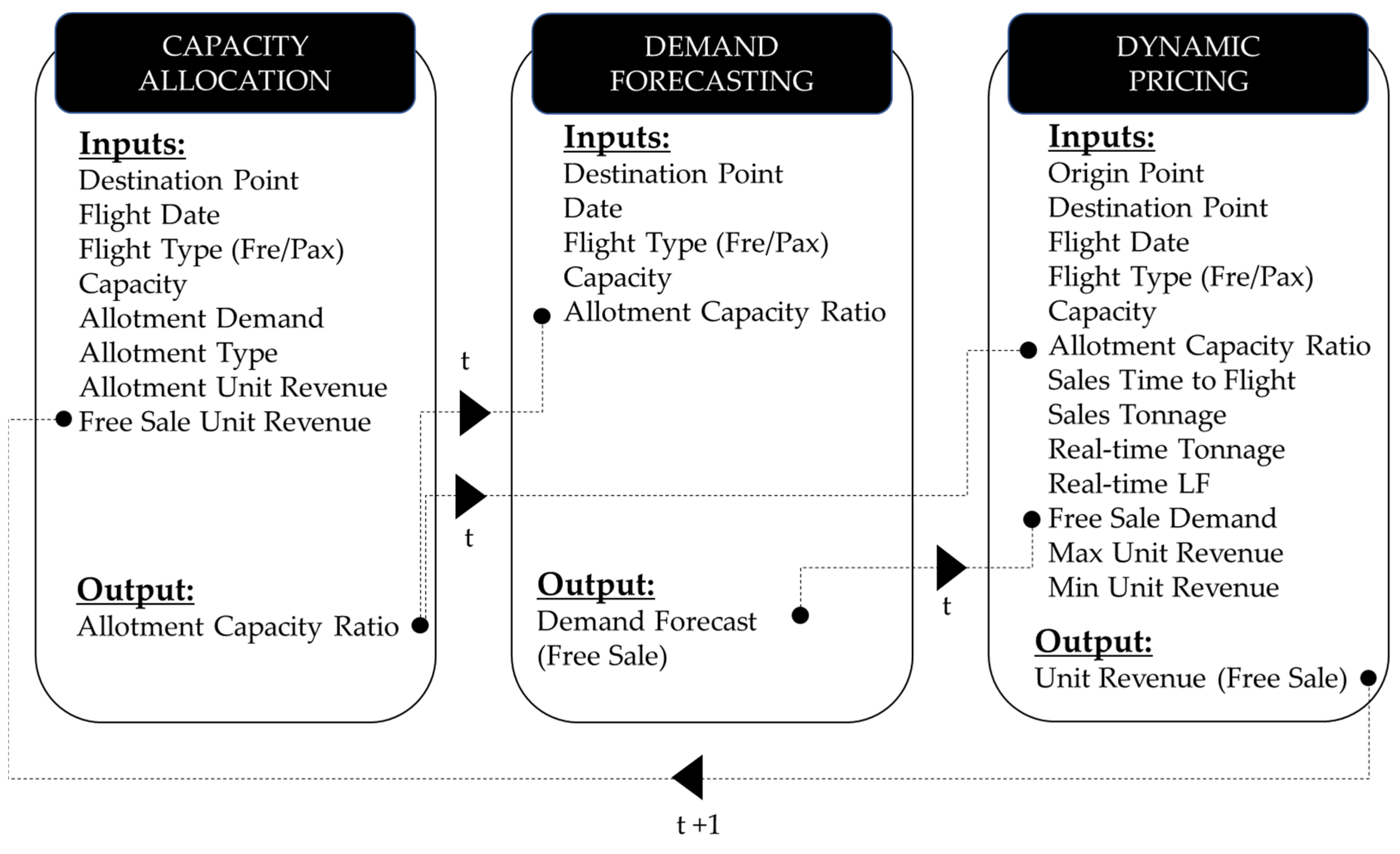
The solution to this optimization problem comprises three primary components: capacity allocation, demand forecasting, and dynamic pricing. In order to determine the model inputs, the existing literature was extensively reviewed, and expert opinions were sought through interviews with the employees of one of the leading air cargo companies in the sector. The interrelation of these three components is illustrated in Figure 2. The model commences with the capacity allocation component, which aims to allocate resources in an efficient manner. The model employed in this stage is derived from the capacity allocation model for the air cargo industry, as published in 2022 [7]. The capacity obtained in this stage serves as the input for both demand forecasting and dynamic pricing. In the subsequent stage, the output of the demand forecasting model serves as the input for pricing. The third stage of the problem resolution is the dynamic pricing of the capacity. The price obtained from the pricing model serves as the input for the capacity allocation section in subsequent periods. Consequently, the objective was to furnish dynamic price recommendations with an integrated structure and an iterative process.

2.1. Capacity Allocation

Air cargo companies can market their capacity through various channels, including free sales and contract sales. Companies can sell their capacities directly to shippers, but they generally sell to forwarders. These forwarders can be allocated capacity on specific routes based on their performance in the previous year. Once a flight is completed, the allocated capacity cannot be used. Therefore, it is imperative to allocate capacity effectively to maximize a company’s profits.

Following the formulation of a plan, there is a possibility that the capacity will be inadequate to fulfill the order on certain routes, while remaining surplus on others [2]. A multitude of factors, including the presence of multiple capacity constraints, variations in capacity, and uncertainty in demand, influence the management of capacity. The company has the option to cancel demand or enter into capacity agreements to mitigate the impact of forwarders canceling their demands. Nevertheless, it remains impractical to entirely eliminate the risk.

Capacity allocation assumes particular importance in circumstances where demand exceeds capacity or when a carrier sells its capacity to multiple carriers [2]. The objective of this study was to propose a solution to the capacity allocation problem. To this end, the study first sought to ascertain the distribution of contracted sales and free sales capacity within the total capacity. For the capacity allocation problem, the study utilized two years of data for four different destinations of one of the successful air cargo companies in the sector. The data were disaggregated monthly for each destination. The creation of the data set and the application of the methods are detailed in the study [7], which includes a capacity allocation model for air cargo in 2022. Two methods were used for capacity allocation: artificial neural network (ANN) and conditional value-at-risk (CVaR). Before proceeding to the model results, the details of the NARX and CVaR methods are given below.

NARX neural network: In 1996, Lin et al. proposed the use of NARX (nonlinear autoregressive exogenous model) for problems where the desired output depends on past data. NARX consists of multiple feedback and forward computation layers and is a dynamic artificial neural network. Compared to traditional feedback network structures, NARX networks show improved learning efficiency [16]. Unlike other feedback networks, NARX networks are characterized by the fact that the feedback is received from the output layer of the neurons and not from all hidden layers. The NARX model can be expressed by the following Equation (1) [17].

y(t) = f(y(t − 1), y(t − 2), …, y(t − ny), x(t − 1), x(t − 2), …, x(t − nx))

(1)

In the equation, y(t − 1), y(t − 2), …, y(t − ny) represents the network outputs, while x(t − 1), x(t − 2), …, x(t − nx) denotes the network inputs. The parameters ny and nx specify the number of previous outputs and inputs, respectively, to be utilized for feedback purposes. The value Y(t), which depends on the output signal, is calculated by combining the signal of the previous output value with the return of the previous independent input signal.

CVaR (conditional value at risk): VaR (value at risk) can be defined as the maximum loss that will occur in a financial asset at a specified time [18]. Accurate VaR measurements can enable businesses to protect themselves against financial risks in advance. In 1999, Philippe Artzner et al. developed the CVaR model in response to criticisms of the VaR method. The CVaR model is fundamentally defined as the expected loss if the potential loss exceeds the value at risk in Equation (2).

CVaR [x] = E {x l x > VaR[x]},

(2)

The calculation of VaR is frequently the subject of critique due to its tendency to produce inconsistent risk measurement results in fat-tailed distributions. A prevailing observation in studies on VaR is the method’s failure to fulfill the sub-layering condition, leading to its classification as an inconsistent risk measure. The subdivision property, an essential component in the definition of a risk measure, is not satisfied by VaR. However, conditional value-at-risk (CVaR) is a consistent risk measure as it satisfies the subdivision property. The CVaR of a portfolio can be defined as the average amount that the portfolio would lose in the worst-case scenario, i.e., X%. On the other hand, VaR can be defined as the best of the worst cases. Rockafeller and Uryasev defined CVaR in Equation (3) [19].

〖CVaR〗_α [X] = 〖min〗_θ ϵ R {θ + 1/(1 − α) E[〖(x − θ)〗₊]},

(3)

The selection of the model to be used as an artificial neural network (ANN) was determined by a series of experiments involving models with different hidden layers, neuron counts, transfer functions, and training functions. The model that yielded the highest R² value was identified as the optimal selection for our study. The results of the tested models can be found in

Table 3. Results produced by different ANN models for capacity allocation.

Network Type	Number of Layers	Number of Neurons	R2
NARX	5	9	54%
NARX	5	10	11%
NARX	6	7	71%
NARX	6	9	41%
NARX	6	10	65%
NARX	7	2	1%
NARX	7	3	35%
NARX	7	5	17%
NARX	7	6	84%
NARX	7	7	33%
NARX	7	8	66%
NARX	7	9	57%
NARX	7	10	93%
NARX	7	11	50%
NARX	8	10	38%

.

To ensure the appropriate allocation of capacity, a statistical evaluation of the results produced by the ANN and CVaR methods was conducted, with a comparison to real data. The statistical results obtained are presented in

Table 4. Statistical comparison of capacity allocation models.

Measure	CVaR Model	ANN Model
ME	−0.229	−0.024
MAD	0.231	0.028
MSE	0.058	0.001
RMSE	0.242	0.032
MNB	−13.856	−1.872
MdAE	0.247	0.028
MAxAE	0.348	0.063
MARE	13.981	1.888
GMAE	0.202	0.021

. An evaluation of the statistical results of the models revealed that the ANN model created using the NARX model yielded superior results. Consequently, the ANN model was employed in the capacity allocation segment of the study.

2.2. Demand Forecasting

Prior to initiating the dynamic pricing model, a demand forecasting model was developed to serve as an input to the model. The inputs utilized by the demand forecasting model were determined through interviews with experts (see Table 1) in the sector who have been employed in this field for an extended period. The resultant inputs for the model were determined as destination point, flight date, aircraft type (passenger or cargo aircraft), total capacity in the relevant period, and capacity allocation rate, which was generated from the capacity allocation model. In order to include economic expectations in the study, an attempt was made to add GDP rates to the model as input. However, since the GDP input did not produce a statistically significant result in the demand forecasting models of the selected destinations, the GDP parameter was removed from the data set. The demand forecast produced in this section will be entered into both the capacity allocation model and the dynamic pricing model.

In order to ensure the proximity of future predictions to reality, it is necessary to select the prediction technique that is suitable for the structure of the problem to be predicted [20]. A taxonomy of forecasting methods can be classified into three broad categories: quantitative forecasting methods, qualitative forecasting methods, and intelligent forecasting methods [21]. Quantitative forecasting methods are based on a thorough analysis of the data, with the input of the method being real data collected at different times. Qualitative forecasting methods, on the other hand, employ the expertise and experience of experts [22]. In certain instances, both qualitative and quantitative methods can be utilized in conjunction. In addition to these conventional methods, intelligent methods such as artificial neural networks (ANNs), genetic algorithms, and fuzzy logic have also been employed in academic literature to predict future outcomes [23]. In our study, we developed a demand forecasting model using historical data. We implemented time series analysis and regression analysis, which are quantitative methods, in our data-based forecasting models. The ANN model, an intelligent method, was employed, and the results of all three models were statistically analyzed. As a result, the model that gave the best results among the tested models was determined.

Regression analysis is a statistical analysis method that has been applied in a wide array of fields, including medicine, chemistry, economics, physics, social sciences, and biology. The objective of regression analysis is to ascertain the relationship between variables (two or more) that may be interrelated. In the model, the variable is divided into two categories: dependent and independent. The variable to be estimated is the dependent variable, while the other variables used to predict the value of the dependent variable are considered independent variables [23]. The selection of independent variables is paramount for optimizing the regression equation, and the relationship between the dependent and independent variables must be meticulously evaluated during analysis. A robust correlation between the dependent and independent variables is essential, and it is equally crucial that the data set is sufficiently large and free of outliers [24].

The structuring of numerical observations in a time-dependent manner is referred to as a time series [25]. The objective of a time series is to construct a model utilizing existing data, with time generally exhibiting equal intervals, such as daily or hourly. Examining the factors influencing realized events facilitates predictions for the future and offers insights into subsequent periods.

Time series analysis is a distinctive analytical method that differs from regression analysis. In time series analysis, the temporal dimension is paramount, as successive observations are typically dependent. This interdependence enables enhanced prediction of future values [26]. When consistent historical data are available, it is feasible to utilize time series analysis methods to model the data and make future predictions. Time series analysis is employed for non-stationary data that exhibits fluctuations over time. Time series analysis is frequently employed in various sectors, including finance, economics, and retail. However, it should be noted that using time series can pose significant challenges because it is difficult to manage market volatility and capture changes in non-stationary data in financial forecasting.

Prior to the selection of an appropriate time series method for our study, a comprehensive investigation was conducted to ascertain the most suitable approach. This investigation entailed a meticulous analysis of the data over a four-year period to discern the characteristics of the series. The findings revealed the presence of comparable patterns in the data on a monthly basis, indicating the existence of a seasonal effect. In addition to the seasonal effect, an upward trend was observed in the demand series. Given the presence of both seasonality and trend in the series, we opted to utilize an exponential smoothing method.

Winters’ method is one of the exponential smoothing methods that can be used when there is a trend, tendency, and seasonality in the series. This method dynamically estimates the trend, the effect of seasonal changes, and cyclical movements. It uses three different correction factors: the correction factor for seasonal variation, the correction factor for cyclical movements, and the correction factor for the trend. Since our data set has seasonality and trend tendency, we chose Winters’ method to use in our model.

In the process of engineering the artificial neural network (ANN) model, a comprehensive evaluation of numerous ANN algorithms was conducted to ascertain their respective degrees of suitability. This evaluation process culminated in the selection of the NARX model for incorporation into our study, a decision that was guided by the observation that the outputs of the NARX model exhibited a greater degree of alignment with the actual data. The tested models’ results can be found in

Table 5. Results produced by different ANN models for demand forecasting.

Network Type	Number of Layers	Number of Neurons	R2
NARX	1	11	86%
NARX	2	8	67%
NARX	2	10	91%
NARX	2	11	91%
NARX	2	12	85%
NARX	3	11	87%
NARX	4	11	89%
NARX	5	11	88%
Feed-Forward Back Propagation Network	2	8	86%
Feed-Forward Back Propagation Network	2	10	87%

.

This study aims to forecast the future demand for the four selected destinations. To this end, the past twenty-four months of data were used to predict four months of data. A total of 627 observations were considered in the data set, and it was found that the results of the time series model yielded the worst R² result when compared to the actual data. Upon examining the data set and its outputs, it was observed that the predictions generated by the time series model were not significantly deficient; however, for a few extreme values, the results exhibited a substantial deviation from the actual data. Consequently, the time series model was modified by excluding these data points, resulting in the acquisition of the corrected time series model results. The statistical outcomes of the multiple regression, time series, and artificial neural network (ANN) models applied to the data set are presented in

Table 6. Statistical comparison of demand forecasting models.

Measure	Multiple Linear Regression	Time Series Winter’s Model	Adjusted Time Series Model	ANN Model
R2	88%	15%	62%	91%
ME	116.880	103.999	175.236	262.918
MAD	183.832	411.765	298.053	289.005
RMSE	229.814	482.661	341.486	338.400

. Following a thorough evaluation of the results, we determined that the multiple linear regression method would be the most suitable approach for our study.

2.3. Dynamic Pricing

Price is one of the most flexible marketing elements, with a direct and short-term impact on a company’s profitability and cost effectiveness. To improve economic and financial performance, companies should define their pricing policies according to a basic systematic understanding of internal capacities and customer needs and wants, as well as market conditions, such as economic conditions and the degree of competition [27]. These multifaceted factors must be meticulously considered during the formulation of dynamic pricing models. In the context of air cargo transportation, a notable example of a dynamic pricing problem arises when attempting to optimize revenue by allocating predefined capacity during a designated planning period, a strategy that necessitates the implementation of dynamic pricing methodologies.

In the field of transport, dynamic pricing practices have been shown to offer advantages to both shippers and carriers. These pricing strategies benefit carriers by reducing transport costs during off-peak periods and by influencing customers to make purchases during these times. This, in turn, contributes to the supply chain by increasing demand. Conversely, carriers are able to maximize their revenue by adapting to market changes and fluctuations in demand through dynamic pricing [28].

The presence of both fixed and variable costs within the sector is a key factor in the determination of pricing strategies. A variety of variable costs, including fuel charges, labor costs, storage costs, and the cost of alternative modes of transport (e.g., land transport, sea transport, etc.) utilized in addition to the flight route for cargo delivery to its final destination, contribute to the overall cost structure. Variable costs exhibit fluctuations in accordance with the volume of cargo, with an increase in cargo volume resulting in a corresponding rise in variable costs.

Du and colleagues [5] incorporated weight and volume capacities, booking type, weight and volume distribution, and cargo type into their dynamic pricing study for air cargo revenue management. Patel et al. [29] incorporated product weight and type, seasonality, distance, origin and destination countries, crude oil price, capacity, and demand inputs into their dynamic pricing model for air cargo transport. Shyr and Lee [30] incorporated a comprehensive set of factors into their study, including demand, priority, cargo type, service quality (e.g., flight frequency, aircraft service reliability), fixed and variable cost of aircraft type, flight distance, flight frequency, capacity, and cargo volume. This study aimed to develop a model for pricing and scheduling strategies for air cargo carriers.

The development of the model incorporated insights from sector experts and a thorough literature review. The route of the flight constitutes the most significant input variable in determining the price, with demand and market conditions along the route exerting an influence on the final price. The model incorporates a range of inputs to ensure comprehensive analysis, including the type of aircraft selected based on its impact on capacity, the date of the flight to account for seasonal variations, the product’s tonnage, and the time remaining until the flight. The model inputs are listed below:

Origin: The city where the sale is made.

Destination: The destination city of the cargo shipped.

Flight type: It is the type of aircraft in which the flight will take place, including passenger and cargo aircraft.

Flight month: The flight was scheduled for the month of the year.

Remaining time to flight: The remaining days indicator ranges from 0 to 30. A value of 0 signifies that the sale was executed on the day of the flight, while higher values indicate subsequent days.

Tonnage: The weight in kilograms of the cargo sold (i.e., the priceable weight)

Capacity: The capacity of the aircraft to perform the flight in terms of weight.

Total tonnage of flight: Total weight of the flight. Actual data for the past period and results from the demand forecast for the future period.

Total load factor: It shows the total load factor of the aircraft. It takes a value between 0 and 1. For the past period, actual data are used, and for the next period, the load factor generated by the results from the demand forecast is used.

Real-time tonnage: Indicates the instantaneous total tonnage on board the aircraft at the time of the sales request.

Real-time load factor: It shows the load factor of the aircraft’s cargo capacity at the time of the sales request. It takes a value between 0 and 1.

Minimum price: It shows the lowest price (USD) that can be offered for the selected departure and destination points during the period in which the flight will take place.

Maximum Price: It shows the highest price (USD) that can be offered for the selected departure and destination points during the period in which the flight will take place.

Revenue: It shows the revenue per AWB (Air Waybill) in USD. Past period data were used to train the model.

The assumptions on which our study is based are as follows:

• Overbooking and cancellations are excluded.
• Discounts are not included in the model.
• The scheduled flight is assumed to operate on the date and route specified.
• Pricing is based on general cargo.
• Pricing of ancillary services is not included in the model.
• It is assumed that market conditions remain stable, excluding trade wars, pandemics, congestion in other modes of transport, and other extraordinary movements that may affect airfreight prices.

The dynamic pricing model is applied to bookings made up to 30 days prior to the scheduled flight.

We need a model that provides real-time pricing recommendations based on the inputs we provide. It is essential that the model can adapt to changing conditions and revise its output accordingly. Before looking at the results of the model, let us look at the SARSA algorithm in more detail.

SARSA algorithm: The goal of reinforcement learning, a machine learning method designed to associate environmental states with actions, is to autonomously make decisions that maximize the expected cumulative payoff. The SARSA algorithm, one of the reinforcement learning algorithms, updates the value of each situation according to the current action and the action to be taken [31]. The basic principle of the algorithm is summarized by the acronym ‘SARSA’, which represents the sequence of events. ‘S—State’, ‘A—Action’, ‘R—Reward’, ‘S—State’, and ‘A—Action’. In the algorithm, an agent connects from a given state and then performs a new action. After the action, it receives a reward and moves to the new state [32]. The computed values for the next state and action pairs are denoted as Q(s, a). A Q table is created with the calculated Q(s, a) values.

An intelligent agent continuously updates the values in the Q-table and interacts with the environment in an iterative process. In this way, the agent makes decisions using probability-weighted greedy strategies that are a combination of the current Q-table values, previous experience, and the current situation [31].

The SARSA algorithm consists of the following steps:

• Initialisation: An initial state is usually chosen randomly, and the action is decided.
• Action implementation: The chosen action is implemented in the environment. The action results in a new state and a reward.
• New action selection: A new action is selected using existing policies.
• Learning: Q-values are updated using past action and new action information. The SARSA algorithm updates the Q-value using the formula in Equation (4) [33].

  Q (s, a) = Q (s, a) + α [r + γQ (s′, a′) − Q (s, a)]

  (4)

  where s is the current state, a is the current action, s′ is the new state, a′ is the new action, r is the reward, α is the learning rate, and γ is the discount factor for future rewards.
• Repetition: The new situation and action are updated as the current situation and action in the next step, and the process of policy formulation is repeated.

The main feature of SARSA is that the Q-values updated at each step of the learning process also include the action choices. Although this makes the learning process more consistent and reliable, it may be less optimistic as the update is based on the chosen action.

The SARSA algorithm can perform better in environments where exploration is important because it takes into account the actual actions performed by the vehicle. It is suitable for scenarios where exploration and exploitation need to be carefully balanced [34]. In machine learning, the SARSA algorithm is used for reinforcement learning and can be applied to natural language processing, image processing, and recommendation systems [35]. The SARSA algorithm follows an exploration and exploitation policy when interacting with the environment and has been used in various areas such as robotic decision-making, path planning problems, and video games [36].

In our study, we used SARSA as a dynamic pricing algorithm. The input and output parameters of the pricing model we created are shown in Figure 3. In the model, we set the state domain as origin, destination, real-time load factor, total load factor, maximum price, minimum price, flight date, time to flight, and tonnage. We set the action domain as the price between the minimum and maximum price and tonnage less than the aircraft capacity. Our objective in the model was to maximize total revenue per flight, and we completed the model by setting this objective as the reward function. Using a reinforcement learning algorithm, we wanted the model to learn using the reward function and provide the most appropriate price recommendation by learning directly through experimentation rather than relying on pre-labeled data. We trained the model on real data. The data set contains four destinations, and a total of ten origin points selling to each destination were examined. Therefore, the total number of origin and destination pairs is 40. When the other inputs (flight date, fleet type, etc.) are added, 25,203 rows of data are obtained. We modeled the model in Python (PyCharm Community Edition) by separating 80% of the data into training and 20% into testing.

In the SARSA algorithm, hyperparameters directly affect the learning process and the behavior of the model. To optimize the performance of the model, we used the grid search method, which is one of the hyperparameter optimization methods. The goal of hyperparameter optimization is to find the hyperparameter combination that maximizes the performance of the model. In our study, we optimized four parameters: alpha (α), gamma (γ), epsilon (ϵ) and number of episodes. To evaluate the performance of the optimization model, the highest total reward was used as the performance measure. Despite the examination of a multitude of origin-destination pairs in the data set according to various fleet types, flight months, sales time to flight, etc., the results were taken as averages for the destinations in order to enhance the comprehensibility of the findings. The hyperparameters we used in the model as a result of the optimization are shown in

Table 7. Hyperparameters used in the model as a result of the grid search method.

Hyperparameters	Value
α	0.1
γ	0.9
ϵ	0.1
Episodes	25.000

.

If we compare the results of the SARSA model with the data allocated for the test on a destination basis, we obtain the results shown in

Table 8. SARSA model results by destination.

Destination	MAE Value
1	1.15
2	0.8
3	0.94
4	0.61

. For destination number four, the model’s price recommendations were closest to the actual prices. Pricing by the system using the established model will help the company to gain manpower, have more control over prices, and generate more revenue. Evaluating the model results, we can say that the model we have built is suitable for use in the air cargo sector to provide dynamic price suggestions. However, the long running time for training the model may be a problem for the real use of the model.

3. Results, Discussion, and Conclusions

We summarize the findings and discuss opportunities for further research. To this end, we have divided the following into two separate sections.

3.1. Methodology and Generalization of Findings

Air cargo management is an important element of modern global logistics and supply chain operations. Air cargo management is a highly complex and challenging endeavor as it requires planning and coordination in many areas. One of these challenging processes is the management of limited cargo capacity. Since the capacity is not available for sale after the flight, it must be sold before the flight. It can be said that air cargo capacity planning is at the forefront of revenue management strategies [37]. There are two main methods of selling capacity: contract sales and free sales.

• Contract sales: Contract sales are agreements between the airline and the customer that guarantee the customer a certain capacity on a certain flight.
• Free sales: There is no allocation of capacity. Capacity is offered for direct sale. There is no guarantee that the capacity will be sold.

Demand forecasting, capacity determination for contract sales, and pricing are some of the important areas of research in revenue management. In air cargo, there are two main dimensions of capacity: weight and volume. For passenger aircraft, the capacity that can be used for carriage is not fixed; it can be affected by the number of passengers, the total amount of baggage, etc. Demand is also different in the two sectors; while passenger demand can be characterized by seasonal fluctuations, on the cargo side, there are many parameters affecting demand, and it is much more difficult to forecast. As a result of all these difficulties, although there are many articles on revenue management in air passenger transport, there are very few on air cargo.

Our first objective in the study is to accurately determine the ratio of allotment capacity for capacity planning. Our second objective is to dynamically price the capacity allocated for free sales. To build the dynamic pricing model, we first built the demand forecasting model.

Capacity management is very critical for the air cargo industry. By allocating capacity correctly, it is possible to increase the load factor and thus the total revenue that can be generated. In the highly competitive air cargo sector, it is essential for companies to get their pricing strategies right in order to stay afloat, gain a competitive advantage, and increase profitability.

In order to correctly perform the capacity allocation, which is the first step of our study, we have built two models, CVaR and ANN. The CVaR model we built is based on the capacity allocation study conducted in 2022 [7]. In our study, we built the CVaR model using GAMS and the ANN model (NARX) using MATLAB (R2024a). We determined the inputs to be used in the ANN model based on a literature review and expert opinion. We compared the model results with real results using two years of data for four different destinations. The R² results were 0.4598 for the CVaR model and 0.9335 for the ANN model. Based on the results, we decided to use the ANN model that we created for the first stage.

In business, dynamic pricing is defined as a strategy that adjusts the price of a product or service in real time based on a variety of factors. Examples of factors that affect price include market demand, seasonality, competitive pressures, and other external factors. The aim of dynamic pricing is to maximize revenue and meet sales targets by charging the highest price customers are willing to pay. By setting a variable price rather than a fixed price, many companies are able to make more profit and offer prices that reflect ever-changing market conditions. In order to provide accurate pricing recommendations, it is essential that the data used in the model is of high quality. For air cargo carriers, dynamic pricing is about filling available capacity with profitable cargo, thus optimizing fleet and resources [5].

In order to build a dynamic pricing model, which is the second objective of the study, the first sub-step is to estimate future demand, which is an important input to the pricing model. Multiple linear regression model, time series model (Winters), and ANN were used to forecast demand. As a result of applying the models using historical data, actual data, and model results were evaluated using many statistical methods. As a result of the evaluation, we decided to use multiple linear regression analysis for demand forecasting as it provides the most appropriate result.

For the dynamic pricing model, we used the output of the capacity allocation model and the demand forecasting model as inputs. In addition to these inputs, we added inputs such as flight time, remaining flight time, cargo weight, aircraft type, and flight route to the model based on literature review and expert opinion. We used the SARSA algorithm for the dynamic pricing model and solved the algorithm using Python. We used 25,203 rows of data to test the accuracy of the model. We used 20% of these data for testing and the remaining data to train the model. Finally, we created an integrated model by using the revenue output of the dynamic pricing model as an input for the capacity allocation model in future periods.

Our model differs from other studies in the literature due to its integrated structure and scope, and the use of a reinforcement learning algorithm for dynamic pricing. The inclusion of expert opinions in the study has helped the model to better reflect real-life situations. The fact that we applied the model using real data from an important airline in the air cargo industry helped us to correctly interpret the model outputs.

As a result of our model and the expert’s thought, the correct allocation of capacity will increase the overall load factor of the aircraft and the revenue to be earned by the company. As a result of the dynamic pricing model we have developed, the system’s automatic pricing will provide the company with labor savings, greater control over pricing, and will help the company to generate more revenue.

3.2. Future Studies

Our suggestions for future studies are separate for capacity allocation and dynamic pricing. For capacity allocation, overbooking, no-shows, and cancelations can be considered in the model. A hybrid model can be built to solve these problems. Overbooking, no-shows, cancelations, and discounts can be added as inputs to the dynamic pricing model. In addition, product type inputs can be added to the model to provide pricing for different product types. To improve the performance of the model, wider ranges of hyperparameters can be used, and different hyperparameter optimization techniques, such as Bayesian optimization, can be tried, compared with other models, and different ANN architectures can be used as well.