Three-Dimensional Borehole-to-Surface Electromagnetic Resistivity Anisotropic Forward Simulation Based on the Unstructured-Mesh Edge-Based Finite Element Method

Abstract

Geophysics is a discipline that studies the properties of subsurface media using physical methods, among which electromagnetic methods have long been an important technical approach in resource exploration. The anisotropy of resistivity in underground media objectively exists in electromagnetic exploration. However, most borehole-to-surface electromagnetic methods (BSEMs) currently process and interpret data based on the assumption of isotropy, which can lead to misinterpretations of observational data in regions where an isotropy is significant. To address this, we propose a 3D edge-based finite element method on unstructured meshes for simulating resistivity anisotropy in BSEMs. A principal-axis anisotropic tensor is introduced to model anisotropy, and the vertical-line transmitter is transformed into an equivalent set of point sources, enabling efficient computation. The accuracy and effectiveness of the proposed numerical algorithm are validated through comparisons with the solutions from Dipole1D and MARE2D. Furthermore, a comparative analysis of reservoir dynamic monitoring under isotropic and anisotropic conditions using the same model reveals that the relative errors in amplitude and phase exceed 40%, and anisotropy must be adequately considered in reservoir monitoring with borehole-to-surface electromagnetic methods. For reservoir models with varying extraction rates, this study further examines the influence of a transmitter’s position on the electromagnetic response characteristics in anisotropic reservoir dynamic monitoring. The results indicate that effective monitoring cannot be achieved when the transmitter is located above the reservoir; however, when the transmitter is positioned below the reservoir, the borehole-to-surface electromagnetic method can significantly enhance the monitoring of reservoir dynamics.

1. Introduction

In the field of geophysical exploration, electromagnetic methods serve as pivotal detection techniques, extensively applied in oil and gas exploration, mineral resource surveys, and groundwater research. These methods infer subsurface structures and their physical parameters by measuring the response of underground media to electromagnetic waves, with resistivity being a key parameter. Traditional electromagnetic approaches typically deploy transmitters and receivers on the surface to capture the electromagnetic (EM) responses of subsurface media. However, due to the diffusive nature of electromagnetic fields, surface-based EM methods often face limitations in detecting deep targets [1]. The borehole-to-surface electromagnetic method emerges as a superior technique for deep exploration, offering advantages unattainable by conventional surface EM methods. This approach involves placing the transmitter within a borehole, in close proximity to the target, emitting electromagnetic signals at various frequencies and measuring the EM response components at the surface to delineate subsurface electrical structures. The reduced distance between the transmitter and the target enhances the clarity of the surface-received EM responses, thereby improving observational accuracy and efficiency [2,3].

In the early development of the borehole-to-surface electromagnetic method, pioneering work was carried out by researchers from the former Soviet Union and Japan. In 1958, based on the methodological framework of downhole seismic exploration, research teams from both countries systematically introduced the concept of joint borehole–surface observations into electromagnetic exploration. This marked the formal proposal of the theoretical concept of “borehole-to-surface electromagnetics” and was accompanied by a landmark experimental validation [4,5]. This innovative, cross-disciplinary technology transfer not only broke through the vertical resolution limitations of traditional surface electromagnetic exploration but also established a solid methodological foundation for the high-precision detection of deep geological structures through the synergistic use of downhole transmitters and surface array receivers. In 2013, Zhdanov et al. [6] employed computer simulations to study CO₂ monitoring at the Kevin Dome sequestration site in Montana, USA, validating the feasibility of the borehole-to-surface electromagnetic method for deep reservoir CO₂ monitoring. Their results demonstrated that the method is not only efficient but also capable of clearly delineating the distribution of CO₂ within subsurface strata [6]. In 2015, Tietze et al. [7] investigated the applicability of borehole-to-surface electromagnetic technology for monitoring fluid movements in German oil fields using a three-dimensional forward modeling approach. Their simulations indicated that the method is highly sensitive to resistivity variations deep within reservoirs and that augmenting the system with downhole acquisition near the reservoir significantly enhances resolution [7]. In 2024, Qin et al. [8] developed a three-dimensional forward modeling code for the borehole-to-surface electromagnetic method using C++ and validated its accuracy and precision by comparing it with semi-analytical solutions. This study further explored the effectiveness and sensitivity of the method in mineral and oil and gas reservoir exploration [8].

Due to computational resource limitations, the current numerical simulation methods for borehole-to-surface electromagnetic techniques generally assume isotropic conditions, which impose certain limitations when describing subsurface media with anisotropic characteristics [9,10]. In reality, factors such as thin-layer deposition or particle alignment in sediments can induce significant variations in the measured data responses owing to the electrical anisotropy present in the Earth’s crust [11,12]. To more accurately characterize the anisotropic properties of subsurface media, in 1996, Wait J.R. et al. analyzed the response of a vertical electric dipole transmitter in layered anisotropic formations [13]. In 2005, Newman et al. conducted detailed studies on the interpretation of deep, complex geological anomalies, warning that the continued use of isotropic models for electromagnetic data interpretation could undermine the reliability of the results [14]. In 2011, Key et al. proposed a parallel, goal-oriented adaptive finite element method for rapidly solving 2.5D controlled-transmitter audio-frequency magnetotellurics (CSAMT) and 2D magnetotellurics (MT) modeling problems, which yielded high-precision solutions and is particularly suited for investigating the response characteristics of CSAMT in media with resistivity anisotropy [15]. Furthermore, in 2017, Wang et al. derived and implemented a three-dimensional staggered-mesh finite difference numerical simulation method for CSAMT with axial resistivity anisotropy [16]. Given that subsurface media often exhibit varying resistivity in different directions, posing challenges for the interpretation of electromagnetic exploration data [17], the development of forward modeling algorithms capable of effectively simulating three-dimensional anisotropic resistivity features is of significant importance.

In the numerical solution of electromagnetic response problems, the finite element method (FEM), the finite difference method (FDM), and the finite volume method (FVM) are the primary numerical techniques [18]. However, the reliance of the FDM on structured meshes limits its application in complex geological models, potentially leading to decreased computational accuracy and erroneous interpretations of predictive parameters [19]. Therefore, the FEM has been increasingly adopted in electromagnetic numerical simulations due to its ability to accurately model complex geological structures using unstructured meshes and enhance the precision of numerical solutions through high-order basis functions [18]. The FEM originated in the field of structural analysis. Although R. Courant et al. provided early mathematical treatment of the method in 1943 [20], it was not until 1968 that the FEM was applied to solve electromagnetic problems [21]. The FEM can be categorized into nodal finite elements and edge-based finite elements. In the nodal finite element method, the degrees of freedom are associated with the nodes of the elements, whereas in the edge-based finite element method, the degrees of freedom are assigned to the edge-based parts within the elements, with the edge-based elements constructed and based on Whitney spaces [22]. The nodal elements enforce both the tangential and normal continuity of edge-based or scalar fields at interface boundaries [23]. However, in edge-based elements, only tangential continuity is enforced at interfaces, aligning with the characteristics of electromagnetic field problems [24]. In electromagnetic analysis, the required continuity is directly achieved using edge-based elements, while in nodal elements, it is obtained through potential formulations [25]. Therefore, when using edge-based elements, field variables can be directly computed, whereas for nodal elements, field variables must be derived from potentials during post-processing [26].

In the finite element method, the most commonly used mesh types are hexahedral [27,28] and tetrahedral meshes [29,30,31]. Among these, tetrahedral meshes are the most prevalent in three-dimensional unstructured meshes, as tetrahedra are the simplest shapes in 3D space and can fill any spatial region [32]. Traditional regular-mesh methods have resolution limitations constrained by mesh density, making it challenging to accurately depict the complex structures of subsurface media [33,34]. Finite element methods based on unstructured meshes can flexibly adapt to the intricate structures of subsurface media, effectively reducing computational complexity and time [35]. Additionally, unstructured-mesh methods offer higher resolution, enabling more precise representation of the complex structures and anisotropic characteristics of subsurface media [36]. Currently, significant research achievements have been made in two-dimensional and three-dimensional anisotropic controlled-transmitter electromagnetic (CSEM) problems using unstructured-mesh finite element methods [37]. However, in the field of borehole-to-surface electromagnetic methods (BSEM), studies that consider resistivity anisotropy within a three-dimensional modeling framework remain relatively limited, particularly those employing edge-based finite element methods on unstructured meshes. While anisotropy has been recognized as a critical factor influencing electromagnetic responses in subsurface formations, most existing research still relies on simplified isotropic assumptions or two-dimensional approximations. The lack of comprehensive 3D numerical approaches that accurately incorporate anisotropic effects, especially in complex geological settings, restricts the applicability and precision of BSEM techniques in real-world reservoir monitoring and subsurface characterization. Therefore, there is a pressing need to develop robust and efficient 3D anisotropic modeling tools tailored to BSEM configurations.

In recent years, several open-transmitter software packages have been developed for the forward and inverse modeling of electromagnetic methods, such as PETGEM [10], custEM [38], SimPEG [39], and emg3d [40]. Among these, PETGEM and custEM utilize tetrahedral meshes and support high-order basis functions. SimPEG employs the finite volume method and supports various mesh types, including staggered meshes, octree meshes, and cylindrical meshes. PETGEM can implement horizontal–vertical resistivity anisotropy, while custEM can achieve principal-axis and full-resistivity anisotropy. These open-transmitter codes provide support for the development of this method.

This study aims to perform three-dimensional numerical simulations of reservoir dynamic monitoring models using the borehole-to-surface electromagnetic method based on an edge-based finite element approach with unstructured meshes. The objective is to evaluate the effectiveness of this method in monitoring reservoir dynamics and to demonstrate its advantages over traditional models that assume resistivity isotropy. To validate the accuracy of the proposed approach, comparisons are made with existing two-dimensional codes capable of handling anisotropic media. Furthermore, this study investigates the electromagnetic response characteristics of anisotropic reservoirs under borehole-to-surface monitoring scenarios.

2. Method

2.1. Governing Equation

The borehole-to-surface electromagnetic response is governed by the diffusive form of Maxwell’s equations, in which the displacement current is neglected and anisotropy is used to characterize the resistivity of complex subsurface media. Specifically, a three-dimensional principal-axis anisotropic resistivity model is considered, and a vertical finite-length-wire transmitter is employed as the excitation transmitter. By assuming a time-harmonic factor of $e^{-i\omega t}$, Maxwell’s equations can be expressed as follows:

$$\nabla \times \mathit{E}=i\omega {\mu }_0\mathit{H}$$

(1)

$$\nabla \times \mathit{H}={\mathit{J}}_{\mathit{S}}+{\mathit{\sigma }}^{*}\mathit{E}$$

(2)

where E represents the electric field, H denotes the magnetic field, $\omega$ is the angular frequency, ${\mu }_0$ is the magnetic permeability of free space, ${\mathit{J}}_{\mathit{S}}$ represents the distribution of the transmitter current, and ${\mathit{\sigma }}^{*}\mathit{E}$ denotes the induced current in the conductive Earth; here, ${\mathit{\sigma }}^{*}$ represents the resistivity tensor, which is given by Equation (3):

$${\mathit{\sigma }}^{*}=\left(\begin{array}{ccc}{\sigma }_{xx}& 0& 0\\ 0& {\sigma }_{yy}& 0\\ 0& 0& {\sigma }_{zz}\end{array}\right)$$

(3)

In electromagnetic exploration, anisotropy is primarily manifested in electrical conductivity. For any anisotropic medium, the conductivity ${\mathit{\sigma }}^{*}$ is a 3 × 3 symmetric and positive-definite tensor, which can generally be obtained by applying a triple Euler rotation to a principal conductivity tensor ${\mathit{\sigma }}^{*}$ [41]. This transformation allows the representation of directional dependencies in conductivity, and it is this tensorial form that distinguishes anisotropic media from isotropic ones, where conductivity is a scalar. Equation (3) explicitly illustrates how anisotropy is introduced into the formulation through this tensor representation.

By substituting Equation (1) into Equation (2), we obtain the following:

$$\nabla \times \nabla \times \mathit{E}+i\omega {\mu }_0{\mathit{\sigma }}^{*}\mathit{E}=i\omega {\mu }_0{\mathit{J}}_{\mathrm{s}}$$

(4)

This approach is known as the curl formulation of the problem [42]. Typically, a primary/secondary field formulation is employed to capture the rapid variations in the primary field without requiring extensive mesh refinement [43]. In this context, it is also referred to as the scattering formulation [44], and the total electric field, E, is expressed as follows:

$$\mathit{E}={\mathit{E}}_p+{\mathit{E}}_{\mathit{s}}$$

(5)

$${\mathit{\sigma }}^{*}={\mathit{\sigma }}_0+\Delta \mathit{\sigma }$$

(6)

Here, ${\mathit{E}}_p$ and ${\mathit{E}}_{\mathit{s}}$ represent the primary and secondary fields, respectively, and ${\mathit{\sigma }}_0$ denotes the background resistivity. For layered models, minor effects are generally neglected in favor of considering only the dominant response ${\mathit{\sigma }}_0$. The primary field, E_p, can be obtained via a semi-analytical solution using Hankel transform filtering [45]. Therefore, we only need to make solutions for the secondary field, which is governed by the following equation:

$$\nabla \times \nabla \times {\mathit{E}}_s+\mathit{i}\omega {\mu }_0{\mathit{\sigma }}^{*}{\mathit{E}}_s=-\mathit{i}\omega {\mu }_0\Delta \mathit{\sigma }{\mathit{E}}_{\mathit{p}}$$

(7)

Meanwhile, homogeneous Dirichlet boundary conditions are imposed, meaning that E = 0 on the boundaries.

By expanding Equation (7) in the X, Y, and Z directions, the differential equations governing the components of the secondary electric field can be obtained as follows:

$${\displaystyle \frac{\partial }{\partial y}}\left({\displaystyle \frac{\partial E_y^s}{\partial x}}-{\displaystyle \frac{\partial E_x^s}{\partial y}}\right)-{\displaystyle \frac{\partial }{\partial z}}\left({\displaystyle \frac{\partial E_x^s}{\partial z}}-{\displaystyle \frac{\partial E_z^s}{\partial x}}\right)-i\omega {\mu }_0{\sigma }_{xx}{E}_x^s=i\omega {\mu }_0\left({\sigma }_{xx}-{\sigma }_0\right)E_x^p$$

(8)

$${\displaystyle \frac{\partial }{\partial z}}\left({\displaystyle \frac{\partial E_z^s}{\partial y}}-{\displaystyle \frac{\partial E_y^s}{\partial z}}\right)-{\displaystyle \frac{\partial }{\partial x}}\left({\displaystyle \frac{\partial E_y^s}{\partial x}}-{\displaystyle \frac{\partial E_x^s}{\partial y}}\right)-i\omega {\mu }_0{\sigma }_{yy}{E}_y^s=i\omega {\mu }_0\left({\sigma }_{yy}-{\sigma }_0\right)E_y^p$$

(9)

$${\displaystyle \frac{\partial }{\partial x}}\left({\displaystyle \frac{\partial E_x^s}{\partial z}}-{\displaystyle \frac{\partial E_z^s}{\partial x}}\right)-{\displaystyle \frac{\partial }{\partial y}}\left({\displaystyle \frac{\partial E_z^s}{\partial y}}-{\displaystyle \frac{\partial E_y^s}{\partial z}}\right)-i\omega {\mu }_0{\sigma }_{zz}{E}_z^s=i\omega {\mu }_0\left({\sigma }_{zz}-{\sigma }_0\right)E_z^p$$

(10)

In the conductivity tensor ${\mathit{\sigma }}^{*}$, the diagonal components ${\sigma }_{xx}$, ${\sigma }_{yy}$, and ${\sigma }_{zz}$ represent the principal conductivities along the x-, y-, and z-directions, respectively. It can be observed that, for a vertically anisotropic medium, although the conductivities along the principal axes differ, the current density in each direction is only related to the conductivity along that corresponding principal axis. Therefore, Equation (7) can still be discretized using the same method as that employed for isotropic media.

2.2. Edge-Based Finite Element Method

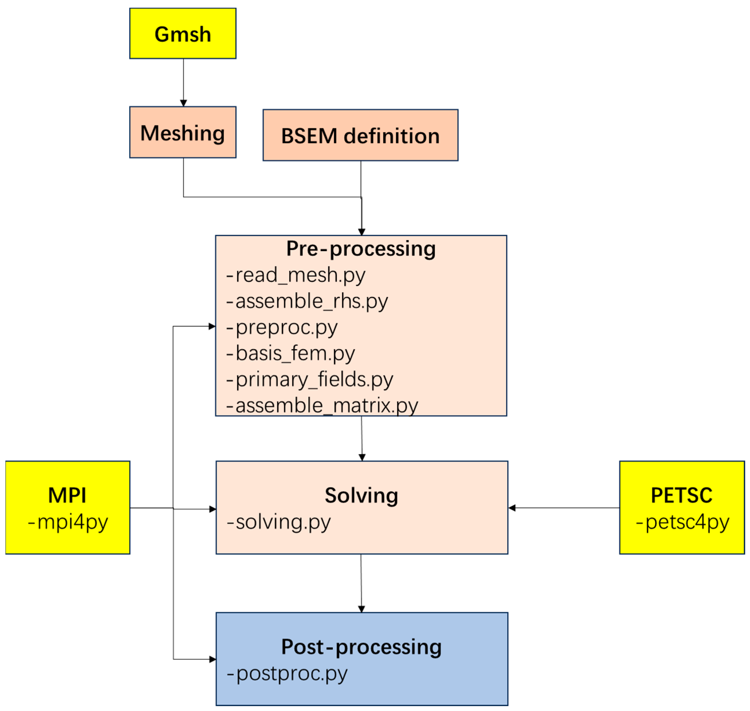
The edge-based finite element method is employed to discretize Equations (8)–(10) using edge-based basis functions ${\mathrm{N}}_{\mathrm{i}}(\mathrm{x}, \mathrm{y}, \mathrm{z})$, which assign edge-based degrees of freedom to the nodes of each element to construct the edge-based finite elements. This approach is particularly well suited for simulating complex geometries and for practical reservoir dynamic monitoring. Moreover, it strikes an excellent balance between accuracy and the number of degrees of freedom, ensuring both computational efficiency and precision.

In the finite element method, the electric field intensity E can be expressed as a linear combination of vector basis functions ${\mathrm{N}}_{\mathrm{i}}(\mathrm{x}, \mathrm{y}, \mathrm{z})$ associated with each edge. The electric field intensity within the tetrahedral element depicted in Figure 1 can be expressed as follows:

$${\mathit{E}}^{\mathit{e}}(x,y,z)=\sum _{i=1}^6{N}_i^e(x,y,z)E_i^e$$

(11)

where $E_i^e$ represents the degree of freedom associated with the i-th edge, and $N_i^e$ is the vector basis function associated with each edge i.

By applying the Galerkin weighted residual method and selecting the test function ${\mathrm{W}}_{\mathrm{i}}(\mathrm{x}, \mathrm{y}, \mathrm{z})={\mathrm{N}}_{\mathrm{i}}(\mathrm{x}, \mathrm{y}, \mathrm{z})$, by substituting the above expression of the electric field into the governing equation, and through derivation, a linear system of equations Kx = b is obtained. Among them are the following:

$$K_{ij}={\displaystyle {\int }_{\mathrm{\Omega }}\left[{\mu }^{-1}\left(\nabla \times N_i^e\right)\cdot \left(\nabla \times N_j^e\right)-\left({\omega }^2\epsilon -i\omega \sigma \right)N_i^e\cdot N_j\right]}d\mathrm{\Omega }+{\displaystyle {\int }_{\partial \mathrm{\Omega }}{r}_t}\left(\widehat{n}\times N_i^e\right)\cdot \left(\widehat{n}\times N_j^e\right)d\mathrm{\Gamma }$$

(12)

$$b_i={\displaystyle {\int }_{\mathrm{\Omega }}{\mathit{J}}_s}\cdot N_i^{e}d\mathrm{\Omega }$$

(13)

where $K_{ij}$ represents the (i, j)-th element of the stiffness matrix, ${\mathit{J}}_s$ denotes the current density of the electric dipole within the tetrahedral element e, and $\widehat{n}$ denotes the unit normal vector at the boundary. To reduce storage space, the large sparse matrix obtained is stored using the Compressed Row Storage (CRS) format. Subsequently, the direct solver from the Portable, Extensible Toolkit for Scientific Computation (PETSc) library is invoked, utilizing the Generalized Minimal Residual (GMRES) solver preconditioned with the Geometric Algebraic Multigrid (GAMG) method to solve the control equations, thereby obtaining the electric field intensity and magnetic induction intensity components on the edges of the mesh elements.

3. Implementation

The code is primarily written in Python 3, relying on the scientific Python (v3.8) software stack for parallel computing through mpi4py [46] and petsc4py [47]. Additional scientific Python packages utilized include NumPy for efficient array operations and SciPy for numerical computations. Furthermore, the algorithm leverages the PETSc library [48] and its extensive data structures and parallel iterative solvers, accessible in Python via petsc4py and mpi4py.

The accuracy and convergence rate of the iterative solver’s solutions heavily depend on the mesh quality. In this study, unstructured meshes are generated using Gmsh (v4.13.1) [49] through the following process (see Figure 2):

• Define the boundary points for the computational domain, as well as the points corresponding to each formation boundary, anomaly boundary, and position of the receivers and transmitters.
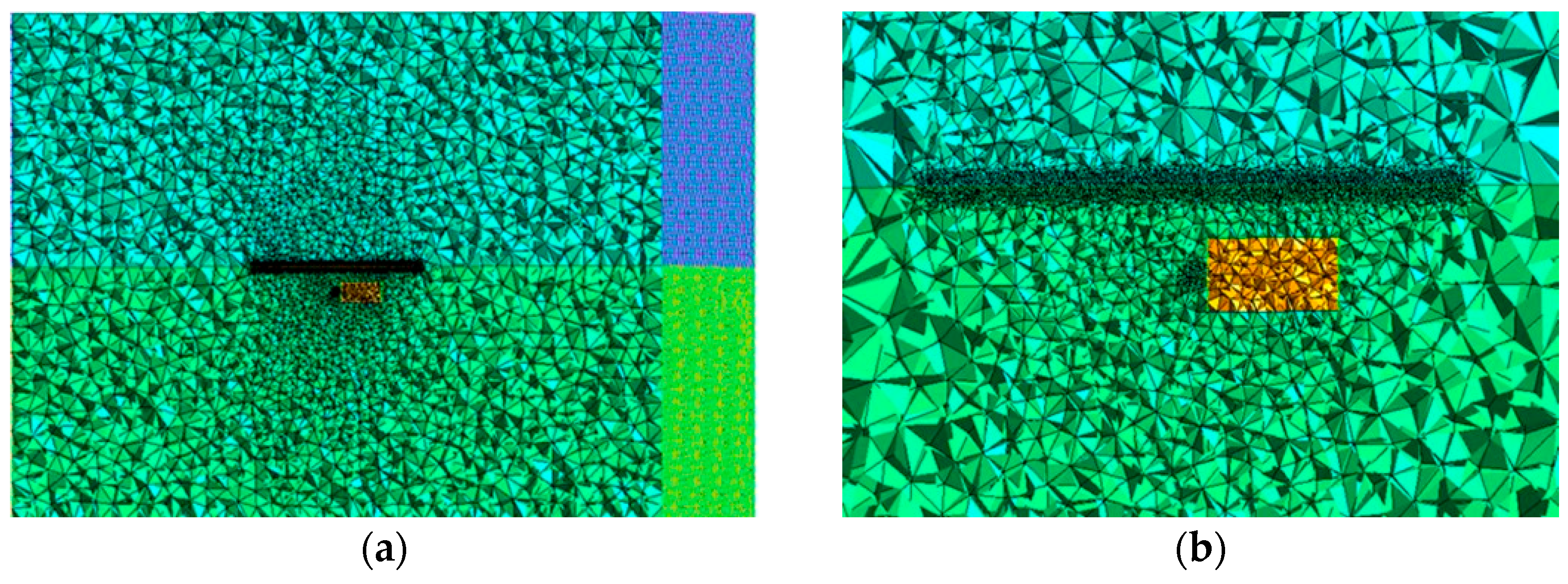
• Connect these points to form lines, surfaces, and volumes, constructing the initial model mesh.
• Refine the mesh around the anomalies, receivers, and transmitter locations.
• Export the final model in msh format for reading by the main program.

Parallelization of the code is achieved through MPI’s efficient communication mechanisms, flexible parallel programming model, and excellent scalability. The computational mesh is partitioned into multiple subdomains, each assigned to an independent process. MPI’s point-to-point and collective communication functions ensure efficient and reliable data transfer between processes. The linear system is correspondingly decomposed, with each process responsible for storing and solving its portion. This strategy not only significantly enhances computational performance and efficiency but also effectively manages large-scale parallel computing tasks.

Once the parameter and model files are defined, the algorithm imports them and begins assembling the global linear system. Kernel generation involves multiple processes, each handling its subdomain to cover the entire computational domain. Each process then assembles its local contributions into the global linear system for solving.

4. Example Verification

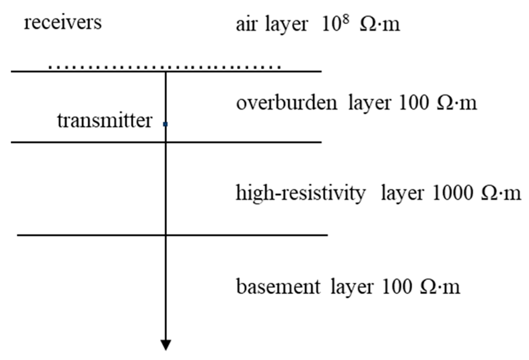
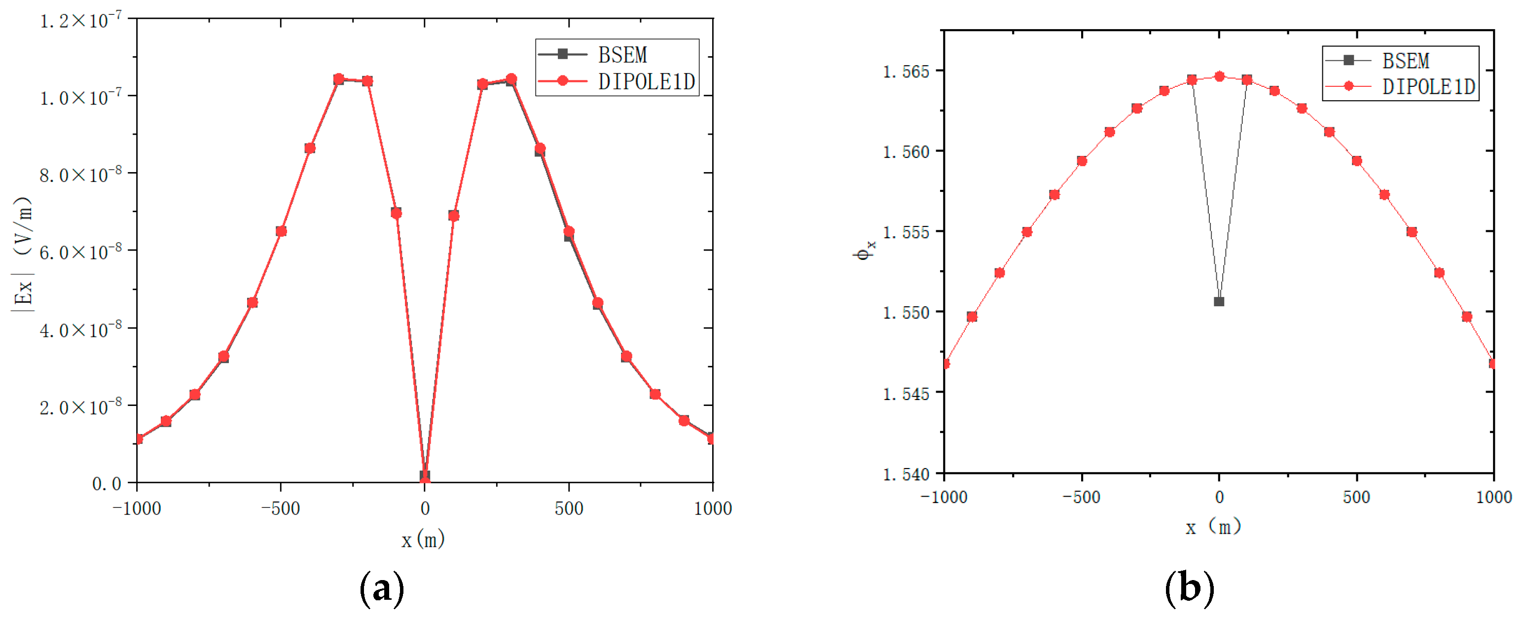
4.1. D Isotropic Reservoir Model

To validate the reliability and effectiveness of the 3D edge-based finite element method for borehole-to-surface electromagnetic modeling under isotropic resistivity conditions, a one-dimensional borehole-to-surface electromagnetic model was established for solutions. The results were compared with those obtained from the semi-analytical solution software DIPOLE1D (v3.13).

As shown in Figure 3, a four-layer one-dimensional stratified reservoir model was established, consisting of an air layer with a resistivity of 10⁸ Ω·m, an overburden layer with a thickness of 1000 m and a resistivity of 100 Ω·m, a high-resistivity reservoir layer with a thickness of 800 m and a resistivity of 1000 Ω·m, and a basement layer with a resistivity of 100 Ω·m. The model was simulated using both the 3D edge-based finite element method with anisotropic resistivity and the semi-analytical solution software DIPOLE1D. A vertical electric dipole transmitter was positioned at a depth of 500 m with transmitter coordinates at (0, 0, −500). The receiver array was deployed along the x-direction, spanning from −1000 m to 1000 m, with a receiver station placed every 100 m, resulting in a total of 21 stations. Given that the typical observation frequency range for borehole-to-surface electromagnetic surveys is 0.1 Hz to 1000 Hz, this study adopts a frequency of 2 Hz for simulations.

Figure 4 shows the unstructured mesh generated using a mesh refinement strategy. The spatial dimensions of the layered model are [−8000, 8000] × [−8000, 8000] × [−5000, 5000]. Figure 4a presents the meshing results generated by Gmsh, where the mesh consists of 334,489 elements, 681,379 faces, and 406,888 edges, with a total of 2,176,534 degrees of freedom.

To verify the performance of the proposed method, the one-dimensional controlled-transmitter electromagnetic forward algorithm proposed by Key was compared with the unstructured 3D edge-based finite element method used in this study, and the response curves were compared. As shown in Figure 5, the simulation results from the proposed algorithm agree well with the one-dimensional analytical solution. Figure 5a presents the amplitude of the electrical response |$E_x$| along the receiver measurement line, clearly indicating that the response results from the unstructured 3D edge-based finite element algorithm match very closely with those from DIPOLE1D. Additionally, the phase of the electrical response was compared, as shown in Figure 5b. Based on this, the relative errors of the amplitude (|$E_x$|) and phase (${\mathrm{\Phi }}_x$) were calculated, as illustrated in Figure 6. The relative errors of the magnitude and phase components of the electric field (Ex) are both less than 1%, proving the correctness of the algorithm in simulating isotropic conditions.

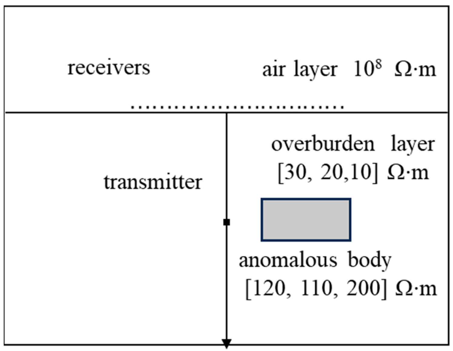
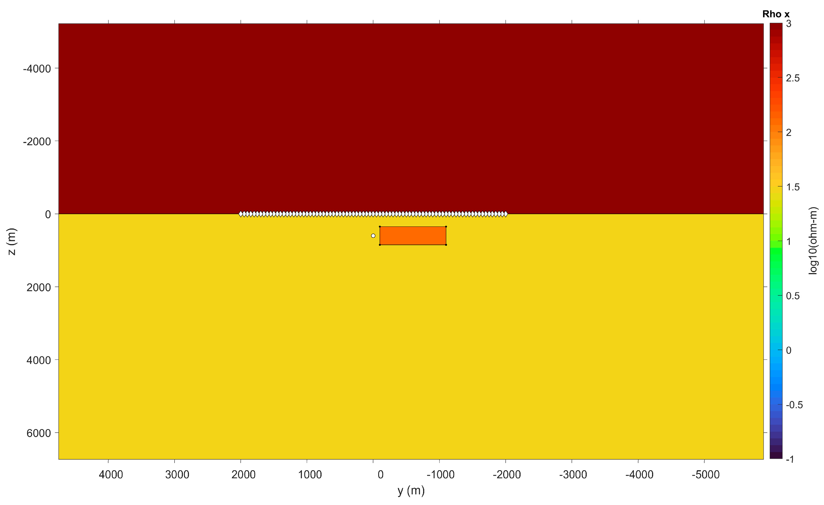
4.2. Two-Dimensional Anisotropic Reservoir Model

To validate the reliability and effectiveness of the borehole-to-surface electromagnetic three-dimensional unstructured vector finite element anisotropic algorithm, a two-dimensional borehole electromagnetic model was established for the algorithmic solution, and the results were compared with those obtained from Key’s 2.5-dimensional adaptive finite element method (MARE2DEM, https://mare2dem.bitbucket.io/master/download.html#).

As shown in Figure 7, the two-dimensional anomaly is rectangular, with a length of 1000 m and a thickness of 500 m (in the three-dimensional model, the width is set to 16,000 m). The center of the anomaly is located at coordinates (600, 0, −600) m, with resistivities of [120, 110, 200] Ω·m. The resistivity of the air layer is set to 10⁸ Ω·m, and the surrounding rock is modeled as a mixture of loose shale and metamorphic rock with resistivities set to [30, 20, 10] Ω·m. The model was simulated using both the borehole-to-surface electromagnetic three-dimensional unstructured finite element anisotropic algorithm (with the computational domain set to [−8000, 8000] [−8000, 8000] [−6000, 6000] m) and MARE2DEM. A 10 m long vertical finite-length-wire transmitter was placed at a depth of 600 m, with the field transmitter coordinates set at (0, 0, −600) m. The measurement line was arranged along the x-direction, with receivers placed every 100 m from −2000 m to 2000 m, resulting in a total of 41 receivers. An observation frequency of 1 Hz was used.

Figure 8 presents a schematic of the two-dimensional reservoir model generated using MARE2D, which employs an integrated mesh adaptation strategy for high-quality discretization. Figure 9a shows the mesh obtained using Gmsh, and Figure 9b illustrates the mesh refinement performed around the transmitter, receivers, and anomaly. The mesh consists of 624,664 elements, 1,261,287 faces, and 743,127 edges, with a total of 4,008,828 degrees of freedom.

In this study, simulations were carried out using both Key’s 2.5-dimensional adaptive finite element method for controlled-transmitter electromagnetic modeling with anisotropy (MARE2DEM) and the borehole-to-surface electromagnetic method based on the unstructured-mesh 3D edge-based finite element anisotropic algorithm (BSEM) proposed in this paper. The response curves obtained from both methods were compared. As shown in Figure 10, the numerical simulation results from our algorithm are in excellent agreement with those from MARE2DEM. Figure 10a displays the amplitude (|$E_x$|) of the electrical response along the receiver line, clearly demonstrating that the responses from the proposed method and MARE2DEM are nearly identical; Figure 10b shows the corresponding phase comparison, with similarly high consistency. Furthermore, the relative errors in amplitude (|$E_x$|) and phase (${\mathrm{\Phi }}_x$) were calculated, as illustrated in Figure 11. The absolute values of the relative errors for the magnitude and phase of the Ex component are less than 5% and 1%, respectively, confirming the reliability of the unstructured-mesh 3D edge-based finite element algorithm under anisotropic conditions.

5. Reservoir Dynamic Monitoring Model

In the previous examples, we demonstrated the correctness of the BSEM. However, a BSEM is also widely used for the dynamic monitoring of oil and gas reservoirs, which are typically characterized by high resistivity. After the extraction of oil and gas, reservoirs are water-filled, leading to lower resistivity [50]. In reservoir dynamic monitoring, resistivity anisotropy is unavoidable due to the combined effects of complex geological structures, variations in rock mineral composition, anisotropic pore structures, differences in fluid saturation, and the impact of human activities [51]. Reservoirs containing thin layers with different resistivities exhibit overall anisotropy, and the differences in resistivity and fluid saturation among these layers further affect the degree of anisotropy. In a reservoir, the resistivity of an individual layer is influenced by capillary effects (typically controlled by grain size) and its elevation relative to the free-water level. In water-wet formations under oil saturation, variations in grain size often result in significant anisotropy [52]. Therefore, it is crucial to fully account for resistivity anisotropy when interpreting monitoring data and optimizing reservoir development strategies.

Based on this, the present study simulated a reservoir beneath the layered strata and designed its dynamic evolution through a layered processing approach. The electromagnetic response variations in the reservoir were computed using the BSEM, thereby enabling the dynamic monitoring of anisotropic reservoirs via borehole electromagnetics. To conduct a simulation study on the dynamic monitoring of anisotropic reservoirs using borehole electromagnetics, a three-dimensional geoelectrical model, as shown in Figure 12, was established for numerical simulation. The model is a four-layer geoelectrical model, with the transmitter moving along the z-axis within two depth intervals: from 500 m to 800 m and from 1200 m to 1500 m. It is assumed that the transmitter emits an electromagnetic signal every 100 m of movement. The electromagnetic data acquisition stations are arranged along the x-axis on the surface, spanning from −4000 m to 4000 m, with a total of 81 receivers, while the transmitter is a vertical-line transmitter of 10 m in length.

As shown in Figure 12, the three-dimensional reservoir model is constructed as a rectangular prism with a length of 3000 m, a width of 2000 m, and a thickness of 400 m. The anomaly is centered at (0, 0, −1000) m with resistivities set to [850, 900, 1000] Ω·m, the air layer’s resistivity is maintained at 10⁸ Ω·m, the first rock layer has resistivities of [10, 20, 30] Ω·m with a thickness of 400 m, the second rock layer has resistivities of [80, 90, 100] Ω·m with a thickness of 1400 m, and the third rock layer has resistivities of [10, 20, 30] with a thickness of 3600 m. The computational domain for the model is [−8000, 8000] × [−8000, 8000] × [−5000, 5000] m. Additionally, the reservoir model is further stratified into upper and lower sections, with the lower part segmented into layers with thicknesses of 0 m, 80 m, 160 m, 240 m, 320 m, and 400 m (as shown in Figure 13), and the resistivity of the lower section is set to [400, 450, 500] Ω·m.

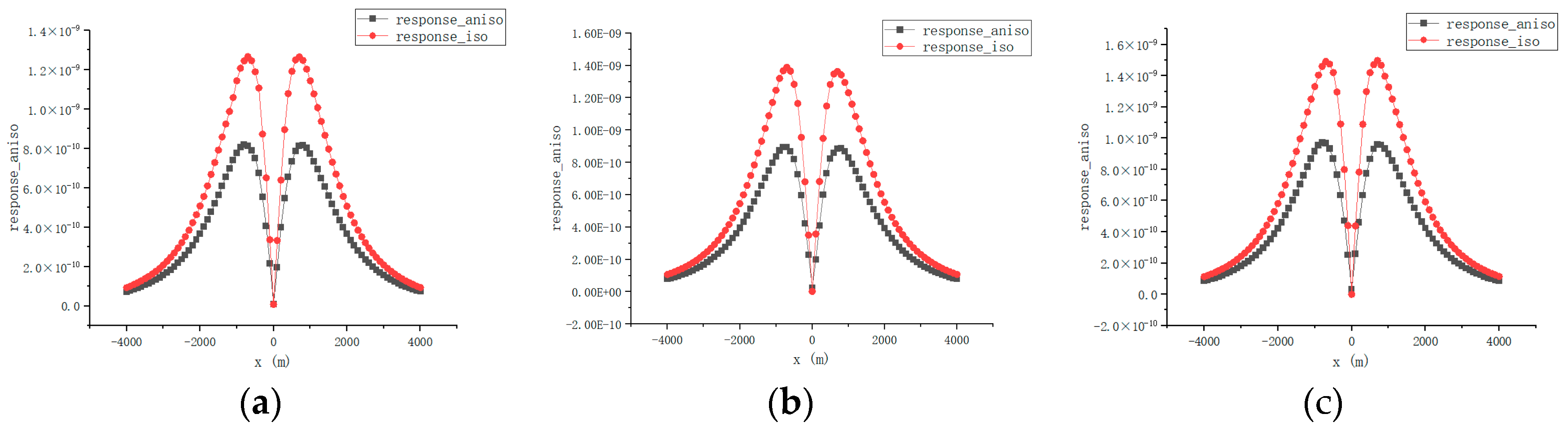
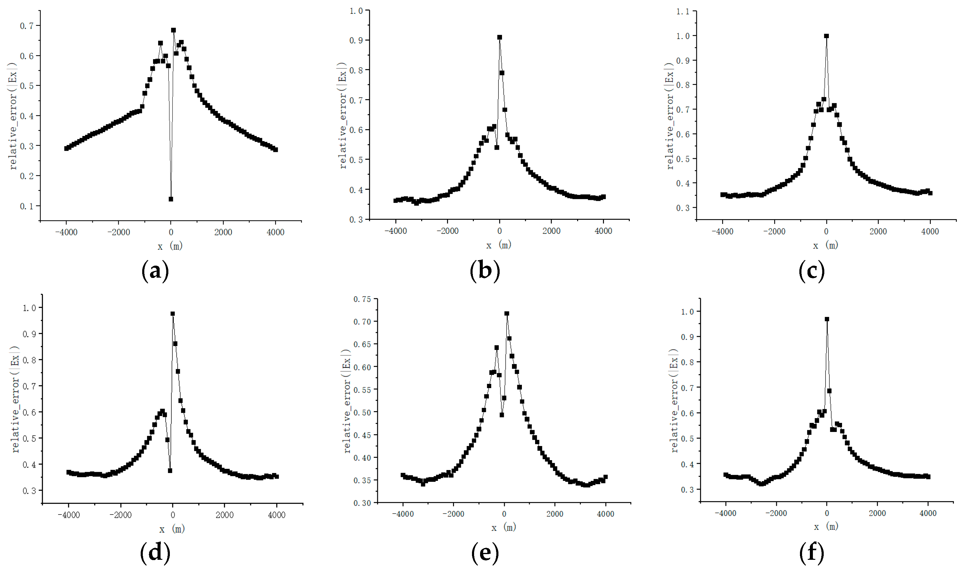
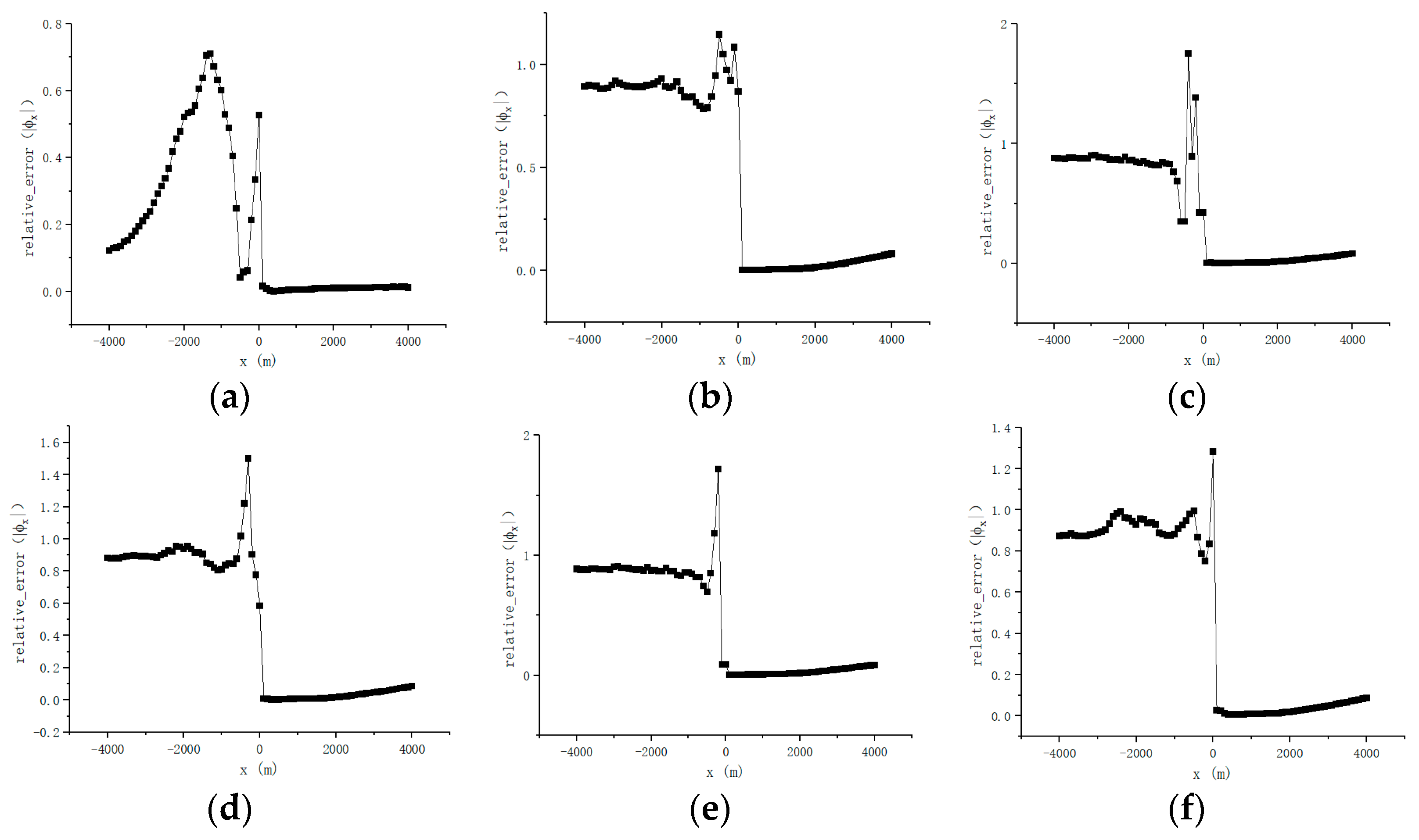
5.1. Comparison of Anisotropic Model and Isotropic Model

In order to demonstrate the significant impact of resistivity anisotropy on reservoir dynamic monitoring, this study constructed an isotropic model alongside the anisotropic model for a comparison and analysis of the differences between the two in reservoir dynamic monitoring. By comparing the calculation results of the isotropic and anisotropic models, this study delves into the influence of resistivity anisotropy on the reliability of reservoir dynamic monitoring.

To obtain the isotropic resistivity corresponding to the anisotropic resistivity, the corresponding expression for isotropic resistivity, based on Equation (3), is as follows:

$$\mathit{\sigma }=\sqrt{{\displaystyle \frac{{{\sigma }_{xx}}^2+{{\sigma }_{yy}}^2+{{\sigma }_{zz}}^2}{3}}}$$

(14)

By substituting the resistivity values from the anisotropic model, the resistivity of the first rock layer is 21.61 Ω·m with a thickness of 400 m, the resistivity of the second rock layer is set to 90.37 Ω·m with a thickness of 1400 m, and the resistivity of the third rock layer is 21.61 Ω·m. The resistivity of the unexploited reservoir is set to 887.41 Ω·m, while the resistivity of the exploited reservoir is set to 451.85 Ω·m. The transmitter is placed at the center of the lower reservoir boundary at coordinates (0, 0, −1200) m, with an emission frequency of 1 Hz.

As shown in Figure 14a–f, when the measurement points extend along the profile from –4000 m to 4000 m, the amplitude gradually decays as the lateral distance |x| increases and reaches its minimum value at the center, exhibiting a typical bimodal distribution. Overall, the amplitude ($\left|E_x\right|$) of the isotropic model is higher than that of the anisotropic model at most measurement points. Additionally, as the reservoir recovery factor increases from 0% to 100%, the amplitude generally shows a progressive increase. A further comparison of the peak values of the curves for both models reveals that as the recovery factor increases, the peak value difference between the isotropic and anisotropic models gradually expands, indicating that the anisotropic effect on the amplitude response becomes more pronounced with an increasing recovery factor.

As shown in Figure 15a–f, the phase variation trends for both the isotropic and anisotropic models generally remain consistent, although there are some local differences. Specifically, in areas far from the reservoir, the phase value of the anisotropic model is slightly higher than that of the isotropic model, while in regions closer to the reservoir, the phase difference between the two models is relatively small. Furthermore, as the recovery factor increases from 0% to 100%, the phase values of both models do not show significant changes, suggesting that the recovery factor has a weak effect on the phase.

Combined with Figure 16a–f and Figure 17a–f, it can be observed that there are significant relative errors in the amplitude and phase values calculated from both the anisotropic and isotropic models, with the average relative error in some local regions approaching 100%. The calculation results show that the average error in amplitude is 42.49%, and the average error in phase is 41.54%. These simulation results indicate that when using the borehole electromagnetic method for reservoir monitoring, the anisotropic effects should be fully considered to improve the accuracy and reliability of the monitoring results.

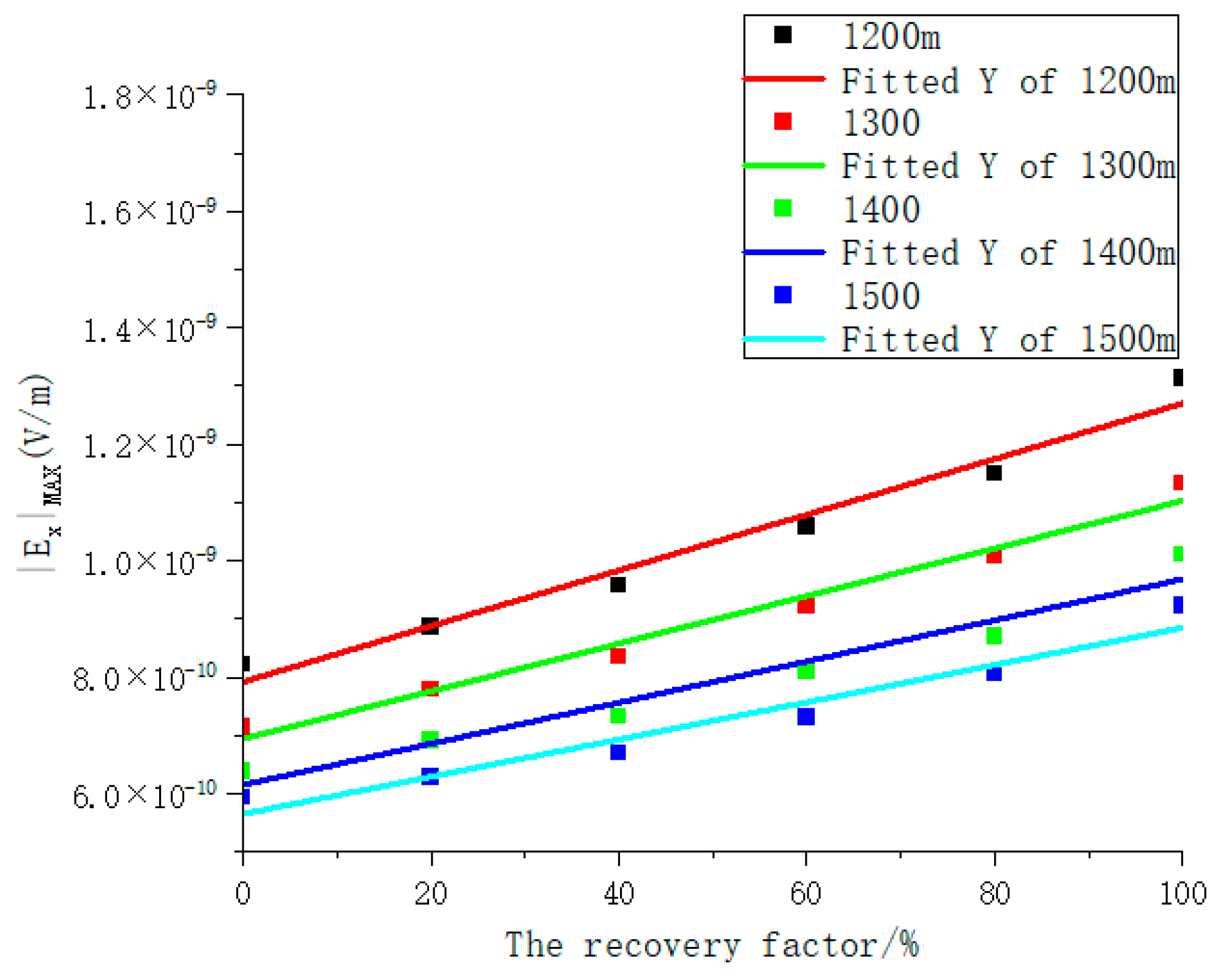
5.2. The Location of the Transmitter

To further investigate the influence of the source position on the effectiveness of reservoir dynamic monitoring, the electromagnetic source is systematically moved along the underground z-axis within the depth ranges of 500–800 m and 1200–1500 m. It is assumed that the source emits an electromagnetic signal at intervals of 100 m, with a transmission frequency set at 1 Hz. Based on this setup, the borehole-to-surface electromagnetic responses of the reservoir under varying extraction levels are computed, with the results presented in Figure 18. Additionally, the maximum amplitude values of the electromagnetic responses at different source depths are sampled, and their variations with extraction levels are statistically analyzed, as shown in Figure 19.

As shown in Figure 18a–d and Figure 19a–d, the maximum amplitude of the electromagnetic response exhibits a positive correlation as the source moves closer to the reservoir. However, when the source is positioned at depths of 500 m, 600 m, or 700 m, the electromagnetic signals received at the surface are minimally influenced by the reservoir, making effective dynamic monitoring infeasible. When the source is placed at the upper boundary of the reservoir, an analysis of the electromagnetic response under different extraction rates reveals that for extraction rates below 20%, the borehole-to-surface electromagnetic method fails to distinguish variations in reservoir depletion. However, once the extraction rate exceeds 20%, the electromagnetic response begins to show a positive correlation with the extraction rate. Furthermore, when the source is positioned below the reservoir, a linear fitting analysis of the maximum amplitude of different electromagnetic components at varying depths (see Figure 20 and

Table 1. Linear fitting curve slopes of the maximum amplitude.

Depth (m)	Linear Fitting Curve Slope
1200	7.8863 × 10−10
1300	6.94106 × 10−10
1400	6.15028 × 10−10
1500	5.65149 × 10−10

) indicates that as the transmitter moves closer to the lower boundary of the reservoir, the slope of the fitting curve increases, suggesting a more pronounced sensitivity of the electromagnetic response to reservoir dynamic monitoring.

6. Conclusions

This study implements a three-dimensional anisotropic numerical simulation of borehole-to-surface electromagnetic responses based on an unstructured-mesh vector finite element method. By leveraging unstructured tetrahedral meshes, the method effectively discretizes small-scale structures and complex geological formations while maintaining computational accuracy and significantly improving efficiency. The accuracy and effectiveness of the proposed algorithm were validated by comparing numerical solutions of a layered isotropic model with semi-analytical solutions and by benchmarking against MARE2DEM solutions for a two-dimensional anisotropic model. The results further underscore the advantages of incorporating resistivity anisotropy over the conventional isotropic assumption.

A comparative numerical study of anisotropic and isotropic reservoirs under varying production rates revealed that the average amplitude error is 42.49%, while the average phase error is 41.54%, highlighting the critical role of anisotropy in reservoir dynamic monitoring. In a three-dimensional geoelectric model, we simulated the BSEM response for anisotropic reservoirs under different production rates and conducted a detailed analysis of the effects of varying transmitter depths on monitoring performance. The results indicate that the effectiveness of reservoir dynamic monitoring varies with the transmitter position. Numerical simulations demonstrate that placing the transmitter closer to the reservoir enhances monitoring sensitivity. When the transmitter is positioned above the reservoir, the received electromagnetic signals on the surface exhibit minimal influence from the reservoir, making precise dynamic monitoring challenging. However, when the transmitter is located at the upper boundary of the reservoir, a positive correlation between the BSEM response and production rate emerges only when the production rate exceeds 20%.

Future studies can incorporate actual geological data to construct more realistic models for further in-depth investigations. The findings of this study provide theoretical and practical contributions to BSEM numerical simulations and offer technical support for oil and gas development and mineral exploration.

References

1. Um, E.S.; Kim, J.; Wilt, M. 3D borehole-to-surface and surface electromagnetic modeling and inversion in the presence of steel infrastructure. Geophysics 2020, 85, E139–E152. [Google Scholar] [CrossRef]
2. He, Z.X. Research to Borehole-Surface Electromagnetic Technique New Way of Mapping Reservoir Boundary. Ph.D. Thesis, Chengdu University of Technology, Chengdu, China, 2006. [Google Scholar]
3. Liu, X.; Wang, J.; He, Z.; Wang, Z. Study of hydrocarbon accumulation by borehole-ground EM method. Progr. Explor. Geophys. 2006, 29, 98–101. [Google Scholar]
4. Paterson, N.R. Experimental and field data for the dual-frequency phase-shift method of airborne electromagnetic prospecting. Geophysics 1961, 26, 601–617. [Google Scholar] [CrossRef]
5. Hedström, E.H.; Parasnis, D.S. Some model experiments relating to electromagnetic prospecting with special reference to airborne work. Geophys. Prospect. 1958, 6, 322–341. [Google Scholar] [CrossRef]
6. Zhdanov, M.S.; Endo, M.; Black, N.; Spangler, L.; Fairweather, S.; Hibbs, A.; Eiskamp, G.; Will, R. Electromagnetic monitoring of CO2 sequestration in deep reservoirs. First Break 2013, 31. [Google Scholar] [CrossRef]
7. Tietze, K.; Ritter, O.; Veeken, P. Controlled-source electromagnetic monitoring of reservoir oil saturation using a novel borehole-to-surface configuration. Geophys. Prospect. 2015, 63, 1468–1490. [Google Scholar] [CrossRef]
8. Qin, C.; Li, H.; Li, H.; Zhao, N. High-order Finite Element Forward Modeling Algorithm for Three-dimensional Bore-hole-to-surface Electromagnetic Method using Octree Meshes. Geophysics 2024, 89, F61–F75. [Google Scholar] [CrossRef]
9. Chen, Q.; Wu, N.; Liu, C.; Zou, C.; Liu, Y.; Sun, J.; Li, Y.; Hu, G. Research progress on global marine gas hydrate resistivity logging and electrical property experiments. J. Mar. Sci. Eng. 2022, 10, 645. [Google Scholar] [CrossRef]
10. Cai, H.; Xiong, B.; Han, M.; Zhdanov, M. 3D controlled-source electromagnetic modeling in anisotropic medium using edge-based finite element method. Comput. Geosci. 2014, 73, 164–176. [Google Scholar] [CrossRef]
11. Guo, H.; Li, Y.; Gong, S.; Lin, L.; Duan, Z.; Jia, S. Three-Dimensional Numerical Simulation of Controlled-Source Electromagnetic Method Based on Third-Type Boundary Condition. Symmetry 2024, 17, 25. [Google Scholar] [CrossRef]
12. Puzyrev, V.; Koldan, J.; de la Puente, J.; Houzeaux, G.; Vázquez, M.; Cela, J.M. A parallel finite-element method for three-dimensional controlled-source electromagnetic forward modelling. Geophys. J. Int. 2013, 193, 678–693. [Google Scholar] [CrossRef]
13. Wait, J.R. Fields of a horizontal wire antenna over a layered half-space. J. Electromagn. Waves Appl. 1996, 10, 1655–1662. [Google Scholar] [CrossRef]
14. Newman, G.A.; Commer, M. New advance in three dimension transient electromagnetic inversion. Geophys. J. Int. 2005, 160, 5–32. [Google Scholar] [CrossRef]
15. Key, K.; Ovall, J. A parallel goal-oriented adaptive finite element method for 2.5-D electromagnetic modeling. Geophys. J. Int. 2011, 186, 137–154. [Google Scholar] [CrossRef]
16. Wang, T.; Wang, K.; Tan, H. Forward modeling and inversion of tensor CSAMT in 3D anisotropic media. Appl. Geophys. 2017, 14, 590–605. [Google Scholar] [CrossRef]
17. Ling, J.; Chen, H.; Wei, S.; Zhang, Y.; Chen, Q.; Liu, S. 3-D resistivity modeling of undulating terrain using space-wavenumber mixed domain approach. Phys. Scr. 2025, 100, 035018. [Google Scholar] [CrossRef]
18. Castillo-Reyes, O.; Modesto, D.; Queralt, P.; Marcuello, A.; Ledo, J.; Amor-Martin, A.; de la Puente, J.; García-Castillo, L.E. 3D magnetotelluric modeling using high-order tetrahedral Nédélec elements on massively parallel computing platforms. Comput. Geosci. 2022, 160, 105030. [Google Scholar] [CrossRef]
19. Shantsev, D.V.; Jaysaval, P.; de la Kethulle de Ryhove, S.; Amestoy, P.R.; Buttari, A.; l’Excellent, J.Y.; Mary, T. Large-scale 3-D EM modelling with a Block Low-Rank multifrontal direct solver. Geophys. J. Int. 2017, 209, 1558–1571. [Google Scholar] [CrossRef]
20. Courant, R. Variational methods for the solution of problems of equilibrium and vibrations. In Finite Element Methods; CRC Press: Boca Raton, FL, USA, 1943. [Google Scholar]
21. Nam, M.J.; Kim, H.J.; Song, Y.; Lee, T.J.; Son, J.; Suh, J.H. 3D magnetotelluric modelling including surface topography. Geophys. Prospect. 2007, 55, 277–287. [Google Scholar] [CrossRef]
22. Nédélec, J.C. Mixed finite elements in R3. Numer. Math. 1980, 35, 315–341. [Google Scholar] [CrossRef]
23. Webb, J.P. Edge elements and what they can do for you. IEEE Trans. Magn. 1993, 29, 1460–1465. [Google Scholar] [CrossRef]
24. Barton, M.L.; Cendes, Z.J. New vector finite elements for three-dimensional magnetic field computation. J. Appl. Phys. 1987, 61, 3919–3921. [Google Scholar] [CrossRef]
25. Kamireddy, D.; Madhukar Chavan, S.; Nandy, A. Comparative performance of novel nodal-to-edge finite elements over conventional nodal element for electromagnetic analysis. J. Electromagn. Waves Appl. 2023, 37, 133–161. [Google Scholar] [CrossRef]
26. Lee, J.F.; Sun, D.K.; Cendes, Z.J. Tangential vector finite elements for electromagnetic field computation. IEEE Trans. Magn. 1991, 27, 4032–4035. [Google Scholar] [CrossRef]
27. Kordy, M.; Wannamaker, P.; Maris, V.; Cherkaev, E.; Hill, G. 3-D magnetotelluric inversion including topography using deformed hexahedral edge finite elements and direct solvers parallelized on SMP computers–Part I: Forward problem and parameter Jacobians. Geophys. J. Int. 2016, 204, 74–93. [Google Scholar] [CrossRef]
28. Farquharson, C.G.; Miensopust, M.P. Three-dimensional finite-element modelling of magnetotelluric data with a divergence correction. J. Appl. Geophys. 2011, 75, 699–710. [Google Scholar] [CrossRef]
29. Usui, Y. 3-D inversion of magnetotelluric data using unstructured tetrahedral elements: Applicability to data affected by topography. Geophys. J. Int. 2015, 202, 828–849. [Google Scholar] [CrossRef]
30. Kangazian, M.; Farquharson, C.G. Including geological orientation information into geophysical inversions with unstructured tetrahedral meshes. Geophys. J. Int. 2024, 238, 827–847. [Google Scholar] [CrossRef]
31. Cai, H.; Kong, R.; He, Z.; Wang, X.; Liu, S.; Huang, S.; Kass, M.A.; Hu, X. Joint inversion of potential field data with adaptive unstructured tetrahedral mesh. Geophysics 2024, 89, G45–G63. [Google Scholar] [CrossRef]
32. Zhou, J.; He, K.; Liu, Z.; Ruan, S.; Ran, H.-L. Three-dimensional Finite-Element Forward Modeling and Response Characteristic Analysis of Multifrequency Electromagnetic. Appl. Geophys. 2025, 1–13. [Google Scholar] [CrossRef]
33. Wannamaker, P.E.; Stodt, J.A.; Rijo, L. A stable finite element solution for two-dimensional magnetotelluric modelling. Geophys. J. Int. 1987, 88, 277–296. [Google Scholar] [CrossRef]
34. Li, Y.; Constable, S. 2D marine controlled-source electromagnetic modeling: Part 2—The effect of bathymetry. Geophysics 2007, 72, WA63–WA71. [Google Scholar] [CrossRef]
35. Yin, C.; Hui, Z.; Zhang, B.; Liu, Y.; Ren, X. 3D adaptive forward modeling for time-domain marine CSEM over topographic seafloor. Chin. J. Geophys. 2019, 62, 1942–1953. [Google Scholar]
36. He, G.; Xiao, T.; Wang, Y.; Wang, G. 3D CSAMT modeling in anisotropic media using edge-based finite element method. Explor. Geophys. 2019, 50, 42–56. [Google Scholar] [CrossRef]
37. Yin, C.; Ben, F.; Liu, Y.; Huang, W.; Cai, J. MC-SEM 3D modeling for arbitrarily anisotropic media. Chin. J. Geophys. 2014, 57, 4110–4122. [Google Scholar]
38. Rochlitz, R.; Skibbe, N.; Günther, T. custEM: Customizable finite-element simulation of complex controlled-source electromagnetic data. Geophysics 2019, 84, F17–F33. [Google Scholar] [CrossRef]
39. Cockett, R.; Kang, S.; Heagy, L.J.; Pidlisecky, A.; Oldenburg, D.W. SimPEG: An open source framework for simulation and gradient based parameter estimation in geophysical applications. Comput. Geosci. 2015, 85, 142–154. [Google Scholar] [CrossRef]
40. Werthmüller, D.; Mulder, W.A.; Slob, E.C. emg3d: A multigrid solver for 3D electromagnetic diffusion. J. Open Source Softw. 2019, 4, 1463. [Google Scholar] [CrossRef]
41. Omisore, B.O.; Fayemi, O.; Brantson, E.T.; Jin, S.; Ansah, E. Three-dimensional anisotropy modelling and simulation of gas hydrate borehole-to-surface responses. J. Nat. Gas Sci. Eng. 2022, 106, 104738. [Google Scholar] [CrossRef]
42. Alumbaugh, D.L.; Newman, G.A.; Prevost, L.; Shadid, J.N. Three-dimensional wideband electromagnetic modeling on massively parallel computers. Radio Sci. 1996, 31, 1–23. [Google Scholar] [CrossRef]
43. Cai, H.; Hu, X.; Li, J.; Endo, M.; Xiong, B. Parallelized 3D CSEM modeling using edge-based finite element with total field formulation and unstructured mesh. Comput. Geosci. 2017, 99, 125–134. [Google Scholar] [CrossRef]
44. Zhdanov, M.S. Geophysical Electromagnetic Theory and Methods; Elsevier: Amsterdam, The Netherlands, 2009. [Google Scholar]
45. Anderson, W.L. A hybrid fast Hankel transform algorithm for electromagnetic modeling. Geophysics 1989, 54, 263–266. [Google Scholar] [CrossRef]
46. Dalcin, L.; Fang, Y.L.L. mpi4py: Status update after 12 years of development. Comput. Sci. Eng. 2021, 23, 47–54. [Google Scholar] [CrossRef]
47. Bueler, E. PETSc for Partial Differential Equations: Numerical Solutions in C and Python; Society for Industrial and Applied Mathematics: Philadelphia, PA, USA, 2020. [Google Scholar]
48. Schwarzbach, C.; Börner, R.U.; Spitzer, K. Three-dimensional adaptive higher order finite element simulation for geo-electromagnetics—A marine CSEM example. Geophys. J. Int. 2011, 187, 63–74. [Google Scholar] [CrossRef]
49. Geuzaine, C.; Remacle, J.F. Gmsh: A 3-D finite element mesh generator with built-in pre-and post-processing facilities. Int. J. Numer. Methods Eng. 2009, 79, 1309–1331. [Google Scholar] [CrossRef]
50. Colombo, D.; McNeice, G.W. Quantifying surface-to-reservoir electromagnetics for waterflood monitoring in a Saudi Arabian carbonate reservoir. Geophysics 2013, 78, E281–E297. [Google Scholar] [CrossRef]
51. Passalacqua, H.; Davydycheva, S.; Strack, K. Feasibility of multi-physics reservoir monitoring for Heavy Oil. In Proceedings of the SPE International Heavy Oil Conference and Exhibition, Kuwait City, Kuwait, 10–12 December 2018; p. D032S045R003. [Google Scholar]
52. Klein, J.D.; Martin, P.R. The petrophysics of electrically anisotropic reservoirs. Log Anal. 1997, 38, 25–36. [Google Scholar]
Figure 1. Schematic diagram of an unstructured tetrahedral edge-based element.
Applsci 15 05307 g001
Figure 2. Code structure.
Applsci 15 05307 g002
Figure 3. One-dimensional layered model.
Applsci 15 05307 g003
Figure 4. The y-z section of the mesh for the 1D reservoir model. (a) The schematic diagram of the mesh subdivision; (b) the schematic diagram of the mesh partitioning near the transmitter and receiver.
Applsci 15 05307 g004
Figure 5. Comparison of numerical and analytical solutions for layered model component. (a) Amplitude ( E x ) comparison; (b) phase ( Φ x ) comparison.
Applsci 15 05307 g005
Figure 6. Relative errors of amplitude ( E x ) and phase ( Φ x ) for layered model. (a) Relative error of the amplitude; (b) relative error of the phase.
Applsci 15 05307 g006
Figure 7. Two-dimensional reservoir model.
Applsci 15 05307 g007
Figure 8. MARE2DEM two-dimensional reservoir model.
Applsci 15 05307 g008
Figure 9. Y-Z cross-section of the unstructured mesh for the 2D reservoir model. (a) Overall schematic of the 3D mesh discretization; (b) schematic of the mesh refinement around the transmitter, receivers, and anomaly.
Applsci 15 05307 g009
Figure 10. Component comparison for the 2D anisotropic reservoir model. (a) Amplitude ( E x ) comparison; (b) phase ( Φ x ) comparison.
Applsci 15 05307 g010
Figure 11. Relative errors of amplitude ( E x ) and phase ( Φ x ) for the 2D anisotropic reservoir model. (a) Relative error of the amplitude; (b) relative error of the phase.
Applsci 15 05307 g011
Figure 12. Y-Z cross-section of the unstructured mesh for the 3D reservoir model. (a) Overall schematic of the 3D mesh discretization; (b) schematic of the mesh refinement around the transmitter and receivers.
Applsci 15 05307 g012
Figure 13. Schematic of the 3D reservoir model (red indicates unexploited reservoir layers, blue indicates exploited reservoir layers). (a) The recovery factor is 0%; (b) the recovery factor is 20% extraction; (c) the recovery factor is 40%; (d) the recovery factor is 60%; (e) the recovery factor is 80%; (f) the recovery factor is 100%.
Applsci 15 05307 g013aApplsci 15 05307 g013b
Figure 14. Comparison of the amplitude ( E x ) between the anisotropic model and isotropic model under different recovery factors. (a) The recovery factor is 0%; (b) the recovery factor is 20% extraction; (c) the recovery factor is 40%; (d) the recovery factor is 60%; (e) the recovery factor is 80%; (f) the recovery factor is 100%.
Applsci 15 05307 g014aApplsci 15 05307 g014b
Figure 15. Comparison of the phase ( Φ x ) between the anisotropic and isotropic models at different recovery factors. (a) The recovery factor is 0%; (b) the recovery factor is 20% extraction; (c) the recovery factor is 40%; (d) the recovery factor is 60%; (e) the recovery factor is 80%; (f) the recovery factor is 100%.
Applsci 15 05307 g015
Figure 16. Relative error of amplitude ( E x ) between the anisotropic and isotropic models at different recovery factors. (a) The recovery factor is 0%; (b) the recovery factor is 20% extraction; (c) the recovery factor is 40%; (d) the recovery factor is 60%; (e) the recovery factor is 80%; (f) the recovery factor is 100%.
Applsci 15 05307 g016
Figure 17. Relative error of phase ( Φ x ) between the anisotropic and isotropic models at different recovery factors. (a) The recovery factor is 0%; (b) the recovery factor is 20% extraction; (c) the recovery factor is 40%; (d) the recovery factor is 60%; (e) the recovery factor is 80%; (f) the recovery factor is 100%.
Applsci 15 05307 g017
Figure 18. Response curves of electromagnetic component E x at different transmission depths. (a) Transmitter at 500 m depth, (b) transmitter at 600 m depth, (c) transmitter at 700 m depth, (d) transmitter at 800 m depth, (e) transmitter at 1200 m depth, (f) transmitter at 1300 m depth, (g) transmitter at 1400 m depth, (h) transmitter at 1500 m depth.
Applsci 15 05307 g018
Figure 19. Corresponding curves of maximum amplitude E x f electromagnetic component and extraction rate at different transmission depths. (a) Transmitter at 500 m depth, (b) transmitter at 600 m depth, (c) transmitter at 700 m depth, (d) transmitter at 800 m depth, (e) transmitter at 1200 m depth, (f) transmitter at 1300 m depth, (g) transmitter at 1400 m depth, (h) transmitter at 1500 m depth.
Applsci 15 05307 g019
Figure 20. Linear fitting curve of the maximum amplitude for the transmitter located below the reservoir.
Applsci 15 05307 g020