


MTGNet: Multi-Agent End-to-End Motion Trajectory Prediction with Multimodal Panoramic Dynamic Graph
Abstract
1. Introduction
- A Multimodal Transformer Graph Convolutional Neural Network (MTGNet) is proposed. This network dynamically constructs an agent-centric scene based on vectorization. While capturing global features, it utilizes graph convolutional neural networks to focus on local features and employs a Res_Decoder layer to decode the constructed panoramic vector, which better confirms the established panoramic vehicle connection network;
- A panoramic agent-based fully connected dynamic traffic graph is proposed to solve the resource waste problem caused by building a fixed scene size based on agent-centric methods [4,19,20], and to dynamically divide the traffic scene size. By updating the node features at the current time step through the message-passing mechanism, the changes in the relationships between each agent and other agents at the current time step can be captured, thereby better adapting to the changes in the dynamic environment and local features;
- We propose using a Transformer-based encoder to capture the long-range dependencies among features and filter out noise by leveraging its self-attention mechanism. This approach circumvents the drawbacks of directly using the direct distance between agents as a weight factor to construct the adjacency matrix. It not only reduces the computational overhead of the model but also makes the adjacency relationships of nodes in the panoramic agent fully connected dynamic traffic graph more consistent with the interaction relationships among agents in real traffic scenarios;
- The Argoverse 2.0 dataset [24] was used for testing. Argoverse 2.0 is a fully upgraded version of Argoverse 1.0. It has richer features than Argoverse 1.0. Argoverse 2.0 surpasses Argoverse 1.0 in terms of data scale, diversity, task support, and technical details.
2. Related Studies
3. Methodology
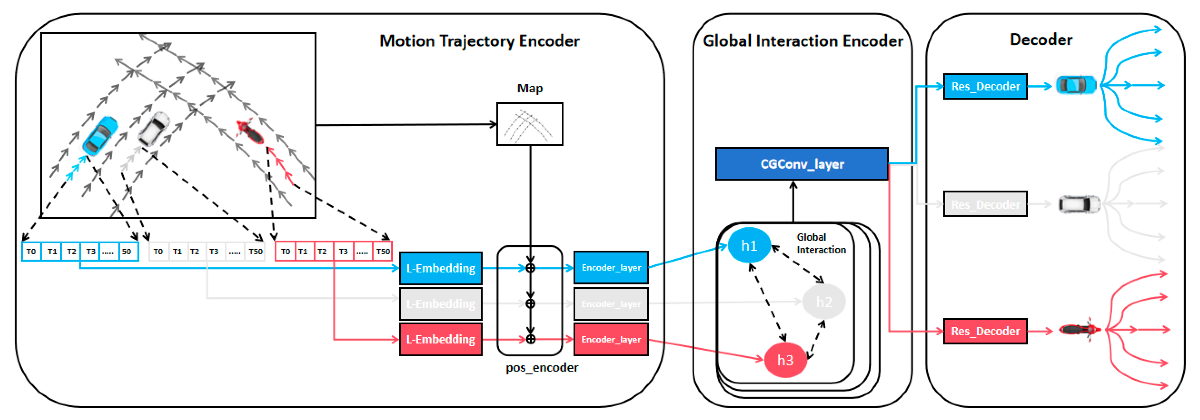
3.1. Overview
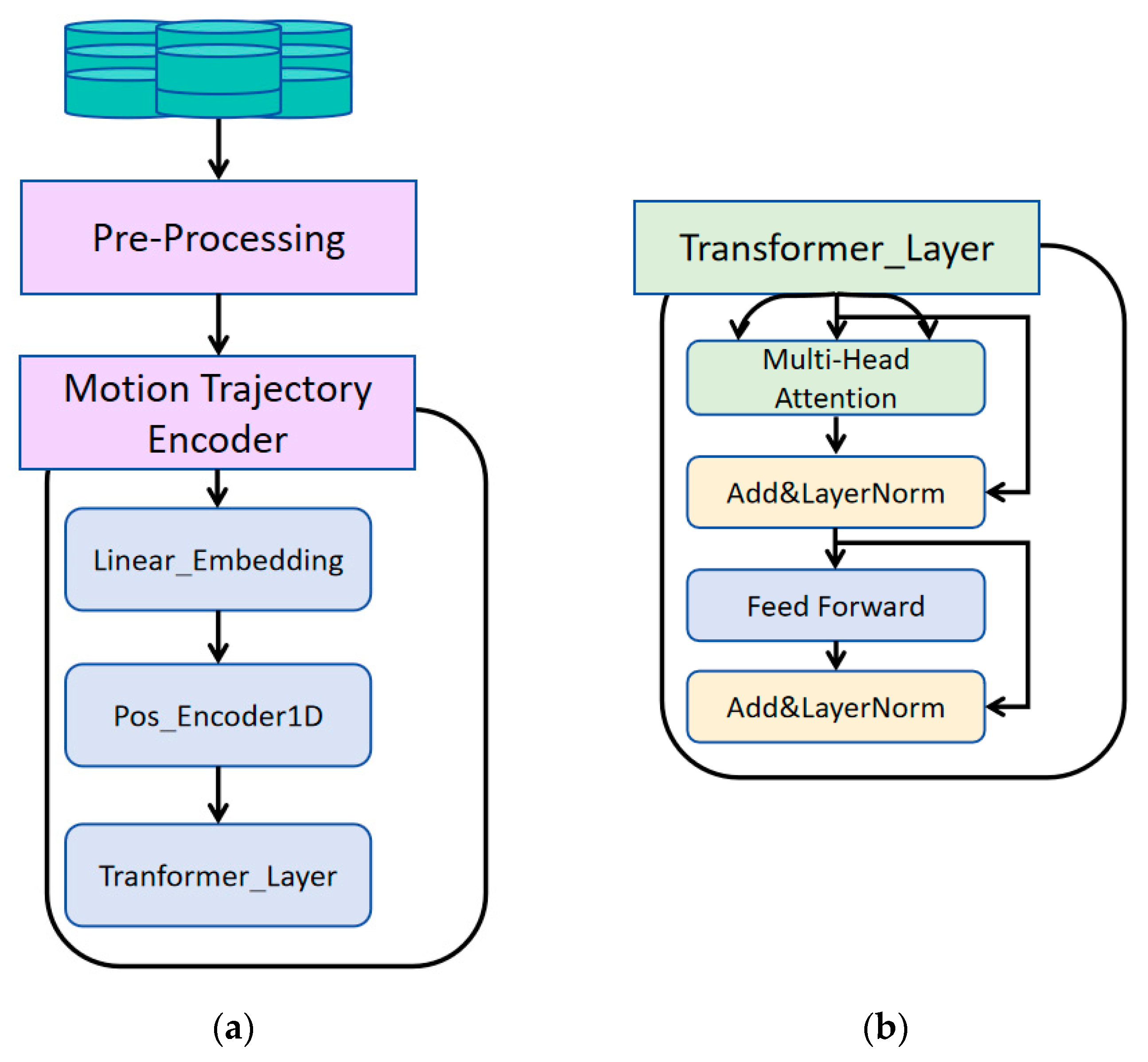
3.2. Motion Trajectory Encoder
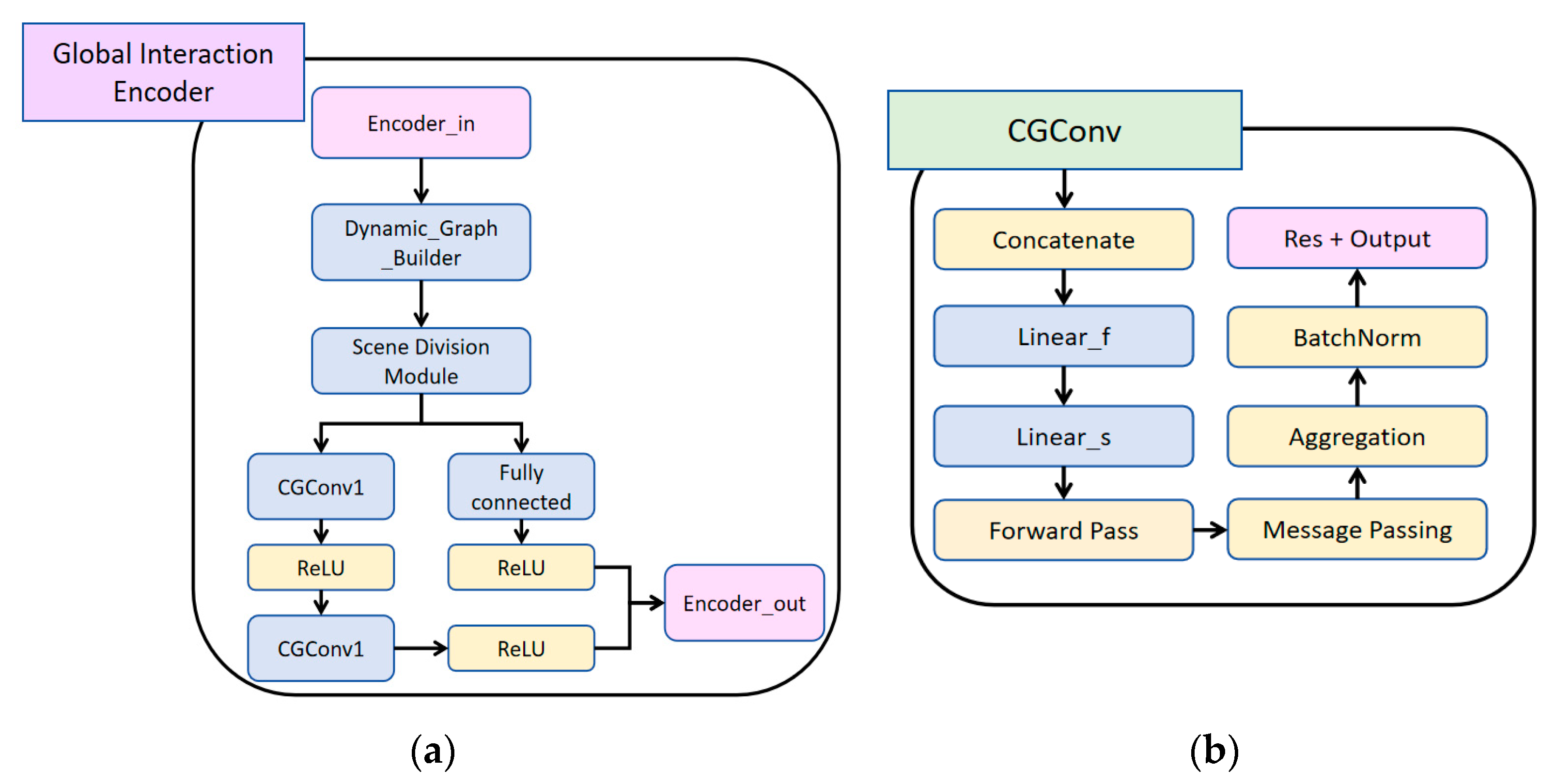
3.3. Global Interaction Encoder
3.4. Decoder
- Panoramic Vector Decoding and Multi-Stage Processing
- Multi-Stage Processing
4. Experimental Results and Analysis
4.1. Experimental Settings
4.1.1. Datasets
4.1.2. Evaluation Indicators
- MR (Miss Rate)
- Brier-minFDE (k = 6)
- denotes the normalized probability of the k-th trajectory for the i-th sample
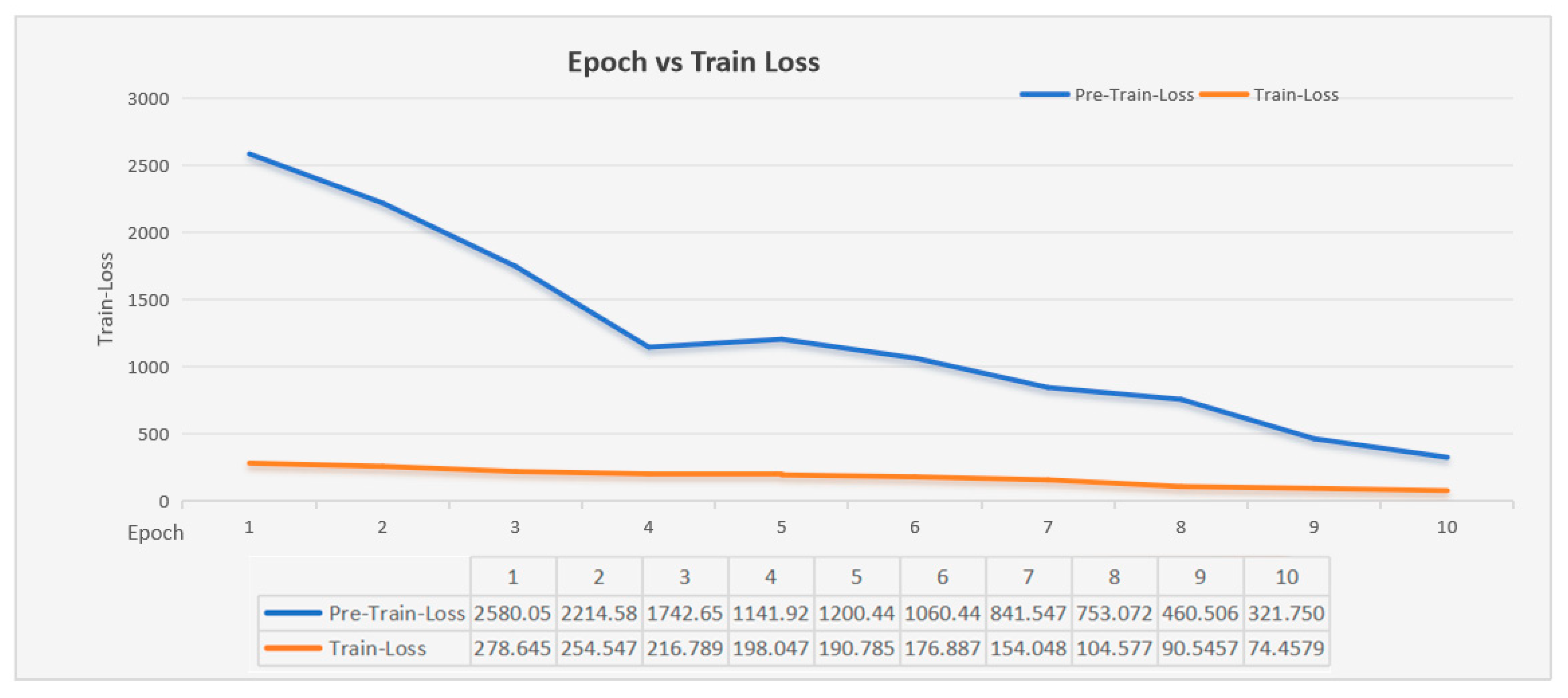
4.1.3. Experimental Details
4.2. Performance Comparison
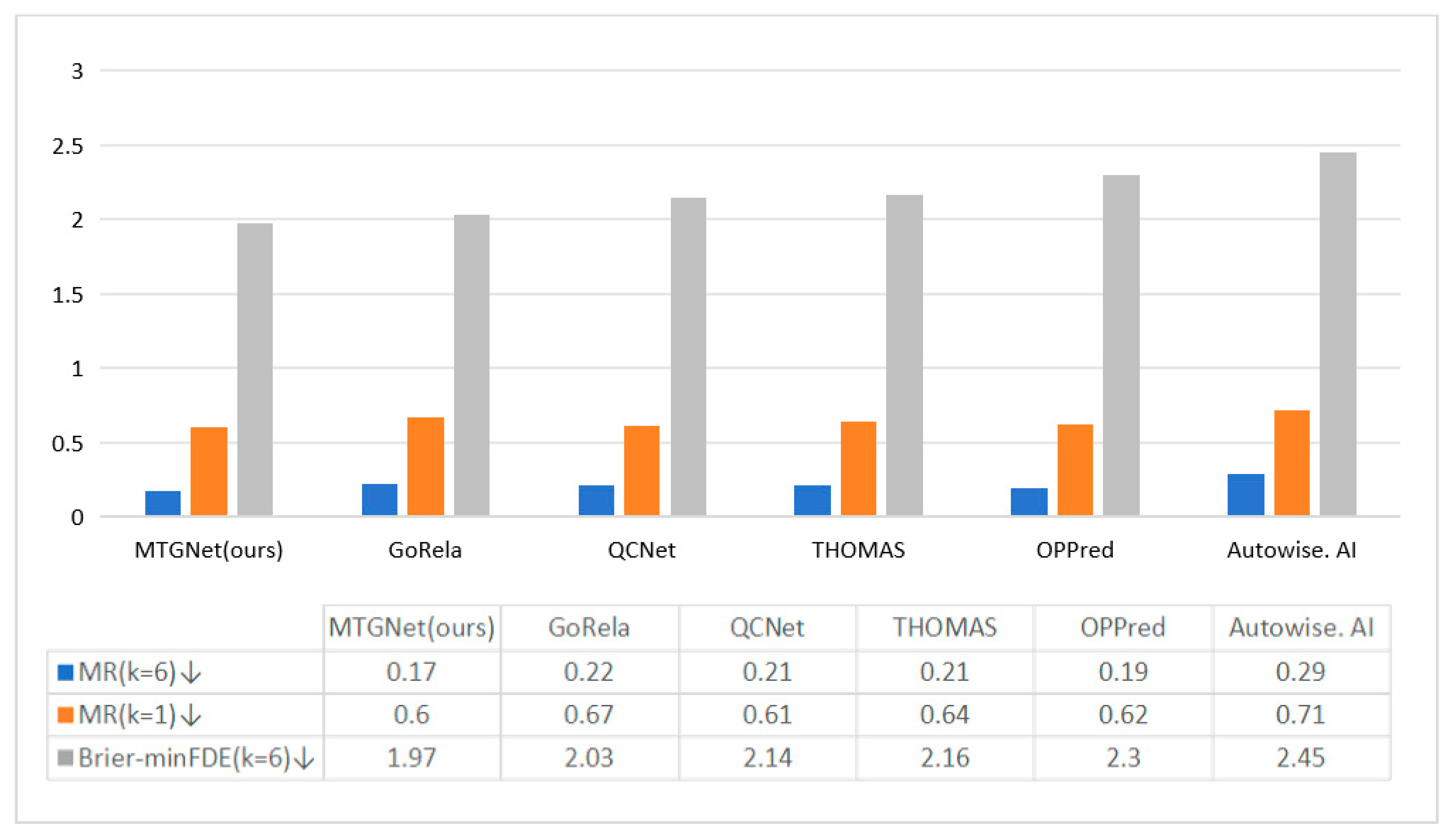
4.2.1. Quantitative Evaluation
4.2.2. Qualitative Evaluation
4.3. Ablation Test
5. Conclusions
Author Contributions
Funding
Institutional Review Board Statement
Informed Consent Statement
Data Availability Statement
Acknowledgments
Conflicts of Interest
Abbreviations
| MTGNet | Multimodal Transformer Graph convolution neural network |
| GCN | Graph Convolutional Neural network |
| CNN | Convolutional Neural Network |
| LSTM | Long Short-Term Memory network |
| RNN | Recurrent Neural Network |
| Bi-RNN | Bidirectional Recurrent Neural Network |
| NLP | Natural Language Processing |
| HiVT | Hierarchical Vector Transformer |
| GRU | Gated Recurrent Unit |
| MR | Miss Rate |
References
- Nayakanti, N.; Al-Rfou, R.; Zhou, A.; Goel, K.; Refaat, K.S.; Sapp, B. Wayformer: Motion forecasting via simple & efficient attention networks. In Proceedings of the 2023 IEEE International Conference on Robotics and Automation (ICRA), London, UK, 29 May–2 June 2023; IEEE: Piscataway, NJ, USA, 2018. [Google Scholar]
- Gilles, T.; Sabatini, S.; Tsishkou, D.; Stanciulescu, B.; Moutarde, F. Thomas: Trajectory heatmap output with learned multi-agent sampling. arXiv 2021, arXiv:2110.06607. [Google Scholar]
- Wei, C.; Hui, F.; Zhao, X.; Fang, S. Real-time Simulation and Testing of a Neural Network-based Autonomous Vehicle Trajectory Prediction Model. In Proceedings of the 2022 18th International Conference on Mobility, Sensing and Networking (MSN), Guangzhou, China, 14–16 December 2022; IEEE: Piscataway, NJ, USA, 2022. [Google Scholar]
- Zhou, Z.; Ye, L.; Wang, J.; Wu, K.; Lu, K. Hivt: Hierarchical vector transformer for multi-agent motion prediction. In Proceedings of the IEEE/CVF Conference on Computer Vision and Pattern Recognition, New Orleans, LA, USA, 18–24 June 2022. [Google Scholar]
- Lin, C.-F.; Ulsoy, A.G.; LeBlanc, D.J. Vehicle dynamics and external disturbance estimation for vehicle path prediction. IEEE Trans. Control Syst. Technol. 2000, 8, 508–518. [Google Scholar]
- Kaempchen, N.; Schiele, B.; Dietmayer, K. Situation assessment of an autonomous emergency brake for arbitrary vehicle-to-vehicle collision scenarios. IEEE Trans. Intell. Transp. Syst. 2009, 10, 678–687. [Google Scholar] [CrossRef]
- Mandalia, H.M.; Salvucci, M.D.D. Using support vector machines for lane-change detection. In Proceedings of the Human Factors and Ergonomics Society Annual Meeting, Orlando, FL, USA, 26–30 September 2005; SAGE Publications: Los Angeles, CA, USA, 2005. [Google Scholar]
- Berndt, H.; Emmert, J.; Dietmayer, K. Continuous driver intention recognition with hidden markov models. In Proceedings of the 2008 11th International IEEE Conference on Intelligent Transportation Systems, Beijing, China, 12–15 October 2008; IEEE: Piscataway, NJ, USA, 2008. [Google Scholar]
- Huang, Y.; Du, J.; Yang, Z.; Zhou, Z.; Zhang, L.; Chen, H. A survey on trajectory-prediction methods for autonomous driving. IEEE Trans. Intell. Veh. 2022, 7, 652–674. [Google Scholar] [CrossRef]
- Deo, N.; Trivedi, M.M. Convolutional social pooling for vehicle trajectory prediction. In Proceedings of the IEEE Conference on Computer Vision and Pattern Recognition Workshops, Salt Lake City, UT, USA, 18–23 June 2018. [Google Scholar]
- Chai, Y.; Sapp, B.; Bansal, M.; Anguelov, D. Multipath: Multiple probabilistic anchor trajectory hypotheses for behavior prediction. arXiv 2019, arXiv:1910.05449. [Google Scholar]
- Kim, B.; Kang, C.M.; Kim, J.; Lee, S.H.; Chung, C.C.; Choi, J.W. Probabilistic vehicle trajectory prediction over occupancy grid map via recurrent neural network. In Proceedings of the 2017 IEEE 20th International Conference on Intelligent Transportation Systems (ITSC), Yokohama, Japan, 16–19 October 2017; IEEE: Piscataway, NJ, USA, 2017. [Google Scholar]
- Hong, J.; Sapp, B.; Philbin, J. Rules of the road: Predicting driving behavior with a convolutional model of semantic interactions. In Proceedings of the IEEE/CVF Conference on Computer Vision and Pattern Recognition, Long Beach, CA, USA, 15–20 June 2019. [Google Scholar]
- Cui, H.; Radosavljevic, V.; Chou, F.-C.; Lin, T.-H.; Nguyen, T.; Huang, T.-K.; Schneider, J.; Djuric, N. Multimodal trajectory predictions for autonomous driving using deep convolutional networks. In Proceedings of the 2019 International Conference on Robotics and Automation (ICRA), Montreal, QC, Canada, 20–24 May 2019; IEEE: Piscataway, NJ, USA, 2019. [Google Scholar]
- Zamboni, S.; Kefato, Z.T.; Girdzijauskas, S.; Norén, C.; Dal Col, L. Pedestrian trajectory prediction with convolutional neural networks. Pattern Recognit. 2022, 121, 108252. [Google Scholar] [CrossRef]
- Sadid, H.; Antoniou, C. Dynamic Spatio-temporal Graph Neural Network for Surrounding-aware Trajectory Prediction of Autonomous Vehicles. IEEE Trans. Intell. Veh. 2024, early access. [Google Scholar] [CrossRef]
- Liang, M.; Yang, B.; Hu, R.; Chen, Y.; Liao, R.; Feng, S.; Urtasun, R. Learning lane graph representations for motion forecasting. In Proceedings of the Computer Vision–ECCV 2020: 16th European Conference, Glasgow, UK, 23–28 August 2020; Proceedings Part II 16. Springer: Berlin/Heidelberg, Germany, 2020. [Google Scholar]
- Gao, J.; Sun, C.; Zhao, H.; Shen, Y.; Anguelov, D.; Li, C.; Schmid, C. Vectornet: Encoding hd maps and agent dynamics from vectorized representation. In Proceedings of the IEEE/CVF Conference on Computer Vision and Pattern Recognition, Seattle, WA, USA, 13–19 June 2020. [Google Scholar]
- Zhou, Z.; Wang, J.; Li, Y.-H.; Huang, Y.-K. Query-centric trajectory prediction. In Proceedings of the IEEE/CVF Conference on Computer Vision and Pattern Recognition, Vancouver, BC, Canada, 17–24 June 2023. [Google Scholar]
- Ridel, D.; Deo, N.; Wolf, D.; Trivedi, M. Scene compliant trajectory forecast with agent-centric spatio-temporal grids. IEEE Robot. Autom. Lett. 2020, 5, 2816–2823. [Google Scholar] [CrossRef]
- Mo, X.; Huang, Z.; Xing, Y.; Lv, C. Multi-agent trajectory prediction with heterogeneous edge-enhanced graph attention network. IEEE Trans. Intell. Transp. Syst. 2022, 23, 9554–9567. [Google Scholar] [CrossRef]
- Su, Y.; Du, J.; Li, Y.; Li, X.; Liang, R.; Hua, Z.; Zhou, J. Trajectory forecasting based on prior-aware directed graph convolutional neural network. IEEE Trans. Intell. Transp. Syst. 2022, 23, 16773–16785. [Google Scholar] [CrossRef]
- Li, H.; Ren, Y.; Li, K.; Chao, W. Trajectory Prediction with Attention-Based Spatial–Temporal Graph Convolutional Networks for Autonomous Driving. Appl. Sci. 2023, 13, 12580. [Google Scholar] [CrossRef]
- Wilson, B.; Qi, W.; Agarwal, T.; Lambert, J.; Singh, J.; Khandelwal, S.; Pan, B.; Kumar, R.; Hartnett, A.; Pontes, J.K. Argoverse 2: Next generation datasets for self-driving perception and forecasting. arXiv 2023, arXiv:2301.00493. [Google Scholar]
- Joseph, J.; Doshi-Velez, F.; Huang, A.S.; Roy, N. A Bayesian nonparametric approach to modeling motion patterns. Auton. Robot. 2011, 31, 383–400. [Google Scholar] [CrossRef]
- Lee, N.; Choi, W.; Vernaza, P.; Choy, C.B.; Torr, P.H.; Chandraker, M. Desire: Distant future prediction in dynamic scenes with interacting agents. In Proceedings of the IEEE Conference on Computer Vision and Pattern Recognition, Honolulu, HI, USA, 21–27 July 2017. [Google Scholar]
- Ma, X.; Tao, Z.; Wang, Y.; Yu, H.; Wang, Y. Long short-term memory neural network for traffic speed prediction using remote microwave sensor data. Transp. Res. Part C Emerg. Technol. 2015, 54, 187–197. [Google Scholar] [CrossRef]
- Xin, L.; Wang, P.; Chan, C.-Y.; Chen, J.; Li, S.E.; Cheng, B. Intention-aware long horizon trajectory prediction of surrounding vehicles using dual LSTM networks. In Proceedings of the 2018 21st International Conference on Intelligent Transportation Systems (ITSC), Maui, HI, USA, 4–7 November 2018; IEEE: Piscataway, NJ, USA, 2018. [Google Scholar]
- Cho, K.; Van Merriënboer, B.; Gulcehre, C.; Bahdanau, D.; Bougares, F.; Schwenk, H.; Bengio, Y. Learning phrase representations using RNN encoder-decoder for statistical machine translation. arXiv 2014, arXiv:1406.1078. [Google Scholar]
- Hou, L.; Xin, L.; Li, S.E.; Cheng, B.; Wang, W. Interactive trajectory prediction of surrounding road users for autonomous driving using structural-LSTM network. IEEE Trans. Intell. Transp. Syst. 2019, 21, 4615–4625. [Google Scholar] [CrossRef]
- Salzmann, T.; Ivanovic, B.; Chakravarty, P.; Pavone, M. Trajectron++: Dynamically-feasible trajectory forecasting with heterogeneous data. In Proceedings of the Computer Vision—ECCV 2020: 16th European Conference, Glasgow, UK, 23–28 August 2020; Proceedings Part XVIII 16. Springer: Berlin/Heidelberg, Germany, 2020. [Google Scholar]
- Vaswani, A.; Shazeer, N.; Parmar, N.; Uszkoreit, J.; Jones, L.; Gomez, A.N.; Kaiser, Ł.; Polosukhin, I. Attention is all you need. Adv. Neural Inf. Process. Syst. 2017, 30. [Google Scholar]
- Dosovitskiy, A. An image is worth 16x16 words: Transformers for image recognition at scale. arXiv 2020, arXiv:2010.11929. [Google Scholar]
- Carion, N.; Massa, F.; Synnaeve, G.; Usunier, N.; Kirillov, A.; Zagoruyko, S. End-to-end object detection with transformers. In Proceedings of the European Conference on Computer Vision, Online Event, 23–28 August 2020; Springer: Berlin/Heidelberg, Germany, 2020. [Google Scholar]
- Zhu, X.; Su, W.; Lu, L.; Li, B.; Wang, X.; Dai, J. Deformable detr: Deformable transformers for end-to-end object detection. arXiv 2020, arXiv:2010.04159. [Google Scholar]
- Roh, B.; Shin, J.; Shin, W.; Kim, S. Sparse detr: Efficient end-to-end object detection with learnable sparsity. arXiv 2020, arXiv:2111.14330. [Google Scholar]
- Chen, L.; Lu, K.; Rajeswaran, A.; Lee, K.; Grover, A.; Laskin, M.; Abbeel, P.; Srinivas, A.; Mordatch, I. Decision transformer: Reinforcement learning via sequence modeling. Adv. Neural Inf. Process. Syst. 2021, 34, 15084–15097. [Google Scholar]
- Jumper, J.; Evans, R.; Pritzel, A.; Green, T.; Figurnov, M.; Ronneberger, O.; Tunyasuvunakool, K.; Bates, R.; Žídek, A.; Potapenko, A. Highly accurate protein structure prediction with AlphaFold. Nature 2021, 596, 583–589. [Google Scholar] [CrossRef] [PubMed]
- Wen, Q.; Zhou, T.; Zhang, C.; Chen, W.; Ma, Z.; Yan, J.; Sun, L. Transformers in time series: A survey. arXiv 2022, arXiv:2202.07125. [Google Scholar]
- Qi, C.R.; Su, H.; Mo, K.; Guibas, L.J. Pointnet: Deep learning on point sets for 3d classification and segmentation. In Proceedings of the IEEE Conference on Computer Vision and Pattern Recognition, Honolulu, HI, USA, 21–26 July 2017. [Google Scholar]
- Guo, C.; Fan, S.; Chen, C.; Zhao, W.; Wang, J.; Zhang, Y.; Chen, Y. Query-Informed Multi-Agent Motion Prediction. Sensors 2023, 24, 9. [Google Scholar] [CrossRef] [PubMed]
- Bharilya, V.; Kumar, N. Machine learning for autonomous vehicle’s trajectory prediction: A comprehensive survey, challenges, and future research directions. Veh. Commun. 2024, 46, 100733. [Google Scholar] [CrossRef]
- Min, H.; Xiong, X.; Wang, P.; Zhang, Z. A Hierarchical LSTM-Based Vehicle Trajectory Prediction Method Considering Interaction Information. Automot. Innov. 2024, 7, 71–81. [Google Scholar] [CrossRef]
- Hu, Z.; Brilakis, I. Matching design-intent planar, curved, and linear structural instances in point clouds. Autom. Constr. 2024, 158, 105219. [Google Scholar] [CrossRef]
- Nair, V.; Hinton, G.E. Rectified linear units improve restricted boltzmann machines. In Proceedings of the 27th International Conference on Machine Learning (ICML-10), Haifa, Israel, 21–24 June 2010. [Google Scholar]
- Veličković, P.; Cucurull, G.; Casanova, A.; Romero, A.; Lio, P.; Bengio, Y. Graph attention networks. arXiv 2017, arXiv:1710.10903. [Google Scholar]
- Wang, Y.; Zhou, H.; Zhang, Z.; Feng, C.; Lin, H.; Gao, C.; Tang, Y.; Zhao, Z.; Zhang, S.; Guo, J. Tenet: Transformer encoding network for effective temporal flow on motion prediction. arXiv 2022, arXiv:2207.00170. [Google Scholar]
- Goodfellow, I.; Bengio, Y.; Courville, A.; Bengio, Y. Deep Learning; MIT Press: Cambridge, UK, 2016; Volume 1. [Google Scholar]
- Cui, A.; Casas, S.; Wong, K.; Suo, S.; Urtasun, R. Gorela: Go relative for viewpoint-invariant motion forecasting. In Proceedings of the 2023 IEEE International Conference on Robotics and Automation (ICRA), London, UK, 29 May–2 June 2023; IEEE: Piscataway, NJ, USA, 2023. [Google Scholar]
- Zhang, C.; Sun, H.; Chen, C.; Guo, Y. Banet: Motion forecasting with boundary aware network. arXiv 2022, arXiv:2206.07934. [Google Scholar]


| Method & Rank | MR (k = 6) ↓ | MR (k = 1) ↓ | Brier-minFDE (k = 6) ↓ |
|---|---|---|---|
| MTGNet (ours) | 0.17 | 0.60 | 1.99 |
| VI LaneIter | 0.19 | 0.60 | 2.00 |
| GoRela [49] | 0.22 | 0.66 | 2.01 |
| OPPred [50] | 0.18 | 0.61 | 2.03 |
| QCNet [19] | 0.21 | 0.60 | 2.14 |
| THOMAS [2] | 0.20 | 0.64 | 2.16 |
| Autowise. AI(GNA) | 0.29 | 0.71 | 2.45 |
| vilab | 0.29 | 0.71 | 2.47 |
| LGU | 0.37 | 0.73 | 2.77 |
| drivingfree | 0.49 | 0.72 | 3.03 |
| Method & Rank | Brier-minFDE (k = 6) ↓ | #Param |
|---|---|---|
| MTGNet (ours) | 1.94 | 2148 K |
| HiVT [4] | 2.01 | 2546 K |
| Method | Dynamic Partition Scene | Fully Connected → GCN | Brier-minFDE (k = 6) ↓ |
|---|---|---|---|
| MTGNet | 2.24 | ||
| √ | 2.15 | ||
| √ | 2.20 | ||
| √ | √ | 1.99 |
Disclaimer/Publisher’s Note: The statements, opinions and data contained in all publications are solely those of the individual author(s) and contributor(s) and not of MDPI and/or the editor(s). MDPI and/or the editor(s) disclaim responsibility for any injury to people or property resulting from any ideas, methods, instructions or products referred to in the content. |
© 2025 by the authors. Licensee MDPI, Basel, Switzerland. This article is an open access article distributed under the terms and conditions of the Creative Commons Attribution (CC BY) license (https://creativecommons.org/licenses/by/4.0/).
Share and Cite
Dai, Y.; Zhang, Y.; Zhou, X.; Wang, Q.; Song, X.; Wang, S. MTGNet: Multi-Agent End-to-End Motion Trajectory Prediction with Multimodal Panoramic Dynamic Graph. Appl. Sci. 2025, 15, 5244. https://doi.org/10.3390/app15105244
Dai Y, Zhang Y, Zhou X, Wang Q, Song X, Wang S. MTGNet: Multi-Agent End-to-End Motion Trajectory Prediction with Multimodal Panoramic Dynamic Graph. Applied Sciences. 2025; 15(10):5244. https://doi.org/10.3390/app15105244
Chicago/Turabian StyleDai, Yinfei, Yuantong Zhang, Xiuzhen Zhou, Qi Wang, Xiao Song, and Shaoqiang Wang. 2025. "MTGNet: Multi-Agent End-to-End Motion Trajectory Prediction with Multimodal Panoramic Dynamic Graph" Applied Sciences 15, no. 10: 5244. https://doi.org/10.3390/app15105244
APA StyleDai, Y., Zhang, Y., Zhou, X., Wang, Q., Song, X., & Wang, S. (2025). MTGNet: Multi-Agent End-to-End Motion Trajectory Prediction with Multimodal Panoramic Dynamic Graph. Applied Sciences, 15(10), 5244. https://doi.org/10.3390/app15105244