Research on Path Planning Multiple Mobile Robots Based on the LAPGWO Algorithm

Abstract

Given that the traditional optimization algorithm (GWO) often encounters problems like local optimum, and the convergence efficiency is not satisfactory in the path planning task of multiple mobile robots, an improved grey wolf optimization algorithm (LAPGWO) based on the combination of the logistic chaotic mapping and the artificial potential field method (APF) is proposed. Firstly, the LAPGWO algorithm uses logistic chaotic mapping to initialize the scale of grey wolves, improving the diversity of the population distribution. Secondly, the potential field function of APF is introduced to guide the individual grey wolves to move towards the low potential energy area. By adjusting the angle between the resultant force direction of the possible field and the movement direction, the global search ability is enhanced, and the algorithm is prevented from falling into the local optimum. At the same time, in the later iterations, it gradually decreases to increase the local search ability and accelerate the search efficiency. Finally, a repulsive force correction term function is proposed to solve the problem of unreachable targets. An independent potential field is constructed for each robot during the driving process to reduce path conflicts. To verify the performance of the improved algorithm, this paper will verify and analyze two different improved grey wolf algorithms based on the warehouse environment. The results show that, compared with the GWO algorithm, the shortest path and calculation time of the LAPGWO algorithm is shortened by 22.09%, 34.12%, and 47.75%, respectively. It has better convergence and stability. A physical verification platform is built to verify the practical effectiveness of the method proposed in this paper.

1. Introduction

With the continuous development of artificial intelligence, mobile robots have gradually become prevalent across various fields. Single-mobile robots are struggling to cope with an increasing number of complex environments. As a result, multi-mobile robots have steadily emerged as a current research hotspot [1,2,3,4]. Path planning for multi-mobile robots is one of the primary prerequisites for the system’s successful operation. Reasonable and effective path planning aims to construct a collision-free and shortest (optimal or suboptimal) route between the starting and task points. An optimal path can not only enhance the overall operational efficiency of the system [5,6] but also extend the battery life of robots by reducing costs. Moreover, it reserves decision-making space for responding to sudden tasks.

Path planning methods for multi-robot systems can be classified into centralized and distributed categories [7,8,9,10]. Centralized methods generate allocation plans through optimization models based on global information. However, they face high replanning latency and strong communication dependence in dynamic scenarios. Distributed methods achieve autonomous decision making, relying on local interactions, yet they are prone to local–optimum traps and task–conflict risks. Regarding the degree of information mastery of the surrounding environment, path planning can also be divided into global and local path planning [11,12,13]. Most research is dominated by distributed approaches, especially in dynamic large-scale scenarios. This paper will also conduct research using a distributed strategy that combines global and local planning.

2. Related Work

Centralized path planning refers to a full-information collaborative planning approach. Under the premise that the central controller has comprehensive access to environmental information (including obstacle distribution, agent positions, and task objectives), it generates collision-free travel routes for multiple agents through a global optimization model. The planning accuracy of this approach depends on the worldwide modeling ability of the central processor for the environment and the efficiency of multi-objective optimization. Typical algorithms include conflict-based search (CBS) [14], rapidly exploring random trees [15], and hybrid heuristic algorithms [16].

Distributed path planning refers to a collaborative mechanism in which a multi-robot system generates collision-free paths through autonomous decision making based on local environmental perception and neighborhood information interaction without the coordination of a central controller. Its core advantages lie in reducing communication dependence and enhancing adaptability to dynamic environments. Typical methods include distributed model predictive control (DMPC) [17], auction algorithms [18], and swarm intelligence optimization algorithms.

The grey wolf optimization (GWO) [19] algorithm is a new type of bio-inspired algorithm with the advantages of a simple structure, few parameters to set, and easy implementation in experimental coding. In recent years, it has gradually emerged in various fields. However, the traditional GWO algorithm has certain defects, such as the lack of diversity in the initial population, the imbalance between global exploration and local exploitation, the tendency to become trapped in local extrema, and low search efficiency. F Liu [20] proposed a framework that combines GWO with the dynamic window approach (DWA). DWA searches for and optimizes the algorithm’s balance by dynamically adjusting the nonlinear convergence factor. Jiazheng Shen [21] proposed an improved GWO algorithm for the complex three-dimensional environment of vertical farms.

Introducing a grid map hierarchical mechanism and a dynamic priority assignment strategy solves the path conflict problem in multi-robot and multi-task scenarios. Lu [22] proposed a route planning method for military transport aircraft based on the grey wolf optimization (GWO) algorithm. An aviation network model is established by applying the relevant knowledge of graph theory. Then, the GWO algorithm is introduced to optimize the flight path on the constructed aviation network for the route planning of military transport aircraft, resulting in faster convergence speed and higher efficiency. Chengli Hu [23] optimized the GWO algorithm. An optimized numerical intelligent representation of multi-UAV cooperative trajectories using a variable-length coding method is adopted, which reduces the GWO algorithm’s search workload and improves the optimization search’s efficiency. However, the generated path has many redundant paths and is not the optimal one. Huikai Meng [24] proposed a smoothing DGWW global planning method based on the BAS algorithm to optimize the GWO algorithm. This method integrates the optimal search method in the BAS algorithm using the two tentacles of the beetle’s head into the GWO algorithm, thus avoiding local optimization.

However, it increases the calculation time and reduces the search efficiency. Shijie Lu [25] combined the traditional grey wolf optimization (GVO) algorithm with the Coati optimization algorithm (COA) to form the LM-GWO composite algorithm, which successfully planned the best route in a complex marine environment full of obstacles. However, it has a long search time and is prone to becoming trapped in local optima. Hongtao Zhang [26] proposed a multi-population grey wolf optimization (LM-GWO) algorithm based on Levy flight. It combines the idea of multi-population, and clusters individual grey wolves into different populations through the Bi-K-means clustering algorithm. This allows different grey wolf populations to complete different tasks during the training process, thus accelerating the algorithm’s convergence. Gupta Himanshu [27] integrated the Archimedes optimization algorithm with the grey wolf optimizer (GWO) to improve convergence and generate an optimal route in a complex environment. However, it is prone to becoming trapped in local optima and has an extended search time. El Maloufy [28] proposed an optimized algorithm, the chaotic white shark optimizer (CWSO). Integrating chaotic maps into the optimization process is particularly advantageous, as it broadens the search capability, accelerates convergence, and reduces the likelihood of falling into local minima.

El Ghouate [29] proposed the chaotic Kepler optimization algorithm (CKOA). Based on the dynamic diversification strategy of chaotic maps, it is characterized by its ability to better avoid local minima and reach the global optimal solution. It integrates chaotic maps to solve complex engineering problems. Zhixian Li [30] proposed an innovative DRL-MPC-GNNs model, which integrates deep reinforcement learning, model predictive control (MPC), and graph neural networks (GNNs). This improves path planning accuracy, task allocation efficiency, and robot collaborative performance. However, it sacrifices computational time when dealing with complex environments, resulting in lower efficiency.

In response to the deficiencies mentioned above, this paper proposes a solution strategy based on distributed online path planning architecture. By combining the logistic chaotic map with the grey wolf algorithm and introducing the potential field of the artificial potential field method, it aims to find the optimal global path. After the worldwide path search is completed, the artificial potential field method achieves local dynamic obstacle avoidance, realizing the path planning of multiple mobile robots in complex environments. This approach can ensure computational efficiency and, at the same time, guarantee the task completion rate and conflict rate in a multi-mobile robot system. The LAPGWO (the algorithm proposed in this paper), for the first time, deeply integrates the global exploration ability of the chaotic map with the real-time obstacle avoidance characteristics of the APF (artificial potential field), solving the problems of path jitter and the local convergence of traditional GWO variants in scenarios with dynamic obstacles.

The specific contributions are as follows:

1. In the warehouse environment, due to the large number of storage shelves, the initial population of the GWO algorithm fails to distribute evenly, causing the algorithm to miss the global optimal solution in the early stage. To solve this problem, a logistic chaotic mapping method is introduced to enhance the diversity of the population.

2. In the warehouse environment, the GWO algorithm suffers from insufficient global search capabilities, resulting in long search times and low efficiency. To tackle this, we propose introducing factors from the APF method. The attractive potential field accelerates the algorithm’s approach toward the target point, improving the global search capabilities of the GWO algorithm and the system’s efficiency.

3. In the warehouse environment, the abundance of shelf-like obstacles leads to excessive repulsive forces, making it impossible for robots to reach their targets. To address this, a dynamic repulsive potential field function is introduced to solve the problem of unreachable targets. During the movement of robots, collisions with other robots are likely to occur. Thus, each robot’s independent potential field is constructed to avoid collisions. After obstacle avoidance, an attraction function is established based on human shortcut-taking behavior principles to enable robots to return to the preset trajectory smoothly.

3. Methodology

In this section, the path planning method for multiple mobile robots based on the LAPGWO algorithm proposed in this paper is elaborated in detail. This method solves multi-mobile robot path planning problems, such as long global path search time, low efficiency, and the proneness of collisions between robots. Especially in environments with numerous obstacles, it is difficult for robots to quickly and effectively find the optimal path from the starting point to the target point, which minimizes the total cost of all robots completing tasks.

3.1. LAPGWO Algorithm

The purpose of the LAPGWO algorithm is to reduce the impact of complex environments on the efficiency of global path search. Using the logistic chaotic mapping method, the initial distribution of the grey wolf population is improved, the diversity of the population is enhanced, and the possibility of missing the global optimal solution is avoided. Combining with the artificial potential field (APF) method, the grey wolf group can be guided to accelerate the search toward the target point, effectively shortening the search range, reducing the computational workload, and improving efficiency.

3.1.1. GWO Algorithm

The GWO algorithm is a relatively new swarm intelligence optimization algorithm inspired by the predatory behavior of grey wolf packs in nature. Simulating the behaviors of grey wolf packs, such as searching, encircling, and attacking prey, can efficiently solve complex optimization problems. A wolf pack has a relatively straightforward hierarchical system divided into four levels. Among them, the $\mathsf{\alpha }$ wolf is the leader of the group, representing the optimal solution, and is responsible for deciding the hunting direction; the $\mathsf{\beta }$ wolf is the second-best individual, assisting the $\mathsf{\alpha }$ wolf in making decisions, representing the second-best solution; the $\mathsf{\delta }$ wolf is the third-best individual, executing the instructions of the $\mathsf{\alpha }$ and $\mathsf{\beta }$ wolves and is responsible for tasks such as scouting and guarding; the $\mathsf{\omega }$ wolves are ordinary members, following the actions of the former three. The position information of $\mathsf{\alpha }$, $\mathsf{\beta }$, and $\mathsf{\delta }$ guides the entire group to move towards the optimal solution. The predatory behavior of grey wolves is divided into the following three stages: encircling, hunting, and attacking. The mathematical model of the overall predatory behavior of grey wolves can be expressed as follows:

$$X_{(i+1)}=X_p(i)-M·|N·X_p(i)-X(i)|$$

(1)

Among them, $i$ is the iteration number at the current moment. $X$ and $X_p$ are the positions of the grey wolf individual and the prey, respectively. $M$ and $N$ represent vector coefficients, and $M·|N·X_p(i)-X(i)|$ is the Manhattan distance between the position of the grey wolf and the position of the prey.

$$M=2a·r_1-a$$

(2)

$$N=2r_2$$

(3)

Among them, $r_1$ and $r_2$ are random numbers between 0 and 1, and $a$ is the convergence factor, which linearly decreases from 2 during the iterative process until it reaches 0, that is:

$$a(I)=2-2{\displaystyle \frac{i}{i_{max}}}$$

(4)

Among them, $i_{max}$ is the maximum number of iterations.

When the leader wolf $\mathsf{\alpha }$ finds the position of the prey, it commands the entire wolf pack to approach the prey. When the appropriate distance is reached, $\mathsf{\alpha }$ will lead the $\mathsf{\beta }$ wolves and $\mathsf{\delta }$ wolves to launch a joint attack on the prey. Other individuals in the wolf pack will make predictions based on the position information of the three wolves $\mathsf{\alpha }$, $\mathsf{\beta }$, and $\mathsf{\delta }$, and the expression is:

$$\left\{\begin{array}{c}{H}_{\mathsf{\alpha }}=N_1·X_{\mathsf{\alpha }}(i)-X(i)\\ H_{\mathsf{\beta }}=N_2·X_{\mathsf{\beta }}(i)-X(i)\\ H_{\mathsf{\delta }}=N_3·X_{\mathsf{\delta }}(i)-X(i)\end{array}\right.$$

(5)

Among them, $X_{\mathsf{\alpha }}$, $X_{\mathsf{\beta }}$, and $X_{\mathsf{\delta }}$ are the positions of the three wolves $\mathsf{\alpha }$, $\mathsf{\beta }$, and $\mathsf{\delta }$, respectively. $\mathsf{\delta }$, $H_{\mathsf{\beta }}$, and $H_{\mathsf{\delta }}$ are the distances between the three wolves $\mathsf{\alpha }$, $\mathsf{\beta }$, $\mathsf{\delta }$, and other individuals in the group, respectively.

$$\left\{\begin{array}{c}{X}_1(i)=X_{\mathsf{\alpha }}(i)-M_1{H}_{\mathsf{\alpha }}\\ X_2(i)=X_{\mathsf{\beta }}(i)-M_2{H}_{\mathsf{\beta }}\\ X_3(i)=X_{\mathsf{\delta }}(i)-M_3{H}_{\mathsf{\delta }}\end{array}\right.$$

(6)

$$X_{(i+1)}={\displaystyle \frac{X_1(i)+X_2(i)+X_3(i)}{3}}$$

(7)

3.1.2. Improvement and Optimization Based on Logistic Chaotic Mapping

The GWO algorithm uses randomly generated data in the initial map as the position information of the initial population. This random generation method makes it challenging to ensure that the population can cover the entire map, and the grey wolf population cannot be evenly distributed. Therefore, in multi-modal or complex optimization problems, it is easy to miss the global optimal solution. Chaotic mapping has strong randomness and ergodicity, and the chaotic sequence generated by the logistic mapping has even stronger randomness and sensitivity to the initial values, making it suitable for scenarios that require a high perturbation intensity. For this reason, in this paper, the principle of logistic chaotic mapping is selected to generate a uniform chaotic sequence, which is then introduced into the individual search space to develop the individual position sequence in the initial stage of the GWO algorithm. This aims to increase the diversity of the initial population’s position distribution and improve the GWO algorithm’s convergence efficiency. The mathematical expression is as follows:

$$X_{(i+1)}=\mathsf{\mu }·X_i·(1-X_i)$$

(8)

Among them, $X_i\in [0,1]$ represents the state value of the $i$-th iteration, and $\mathsf{\mu }\in [3.57,4]$ represents the chaotic interval. After combining with the GWO algorithm, the initial positions of the population are generated by the logistic chaotic sequence, replacing the traditional uniform random initialization. The expression is as follows:

$$X_t^0=Ib+X_c^{(k)}·(ub-Ib)$$

(9)

Among them, $X_t^0$ represents the initial position of the $t$-th wolf; $X_c^{(k)}$ represents a specific term in the chaotic sequence $X_{(i+1)}$ generated by the logistic mapping iteration, $k$ represents the $k$-th iteration, and $Ib$ and $ub$ represent the lower and upper bounds of the search, respectively.

The search range can be dynamically adjusted by adjusting the value of $\mathsf{\mu }$. In the early search stage, increasing the value of $\mathsf{\mu }$ can enhance the global exploration ability. In the later stage, reducing the value of $\mathsf{\mu }$ can focus on the local area. Meanwhile, during the grey wolves’ position-updating process, logistic chaotic perturbation is introduced to avoid premature convergence. The improved position-updating expression is as follows:

$$X_{(i+1)}={\displaystyle \frac{X_1(i)+X_2(i)+X_3(i)}{3}}+\mathsf{\eta }·X_c^{(i)}$$

(10)

When allocating tasks, the robots’ trajectories in completing them are comprehensively taken into account. The task allocation for each robot should preferably conform to the robots’ spatiotemporal kinematic trajectories. The next task point should preferably be in the same direction as the line connecting the completed task point, forming a joint optimization with the path’s linearity.

The spatiotemporal constraint $S_p$ for the coherence of the robot’s path is as follows:

$$S_p={\displaystyle \frac{\left|\right|V_n·d_k\left|\right|}{\left|\right|V_n\left|\right|·\left|\right|d_k\left|\right|}}·e^{-\mathsf{\beta }·L_d}$$

(11)

Among them, $\mathsf{\eta }$ is the perturbation intensity coefficient, and $X_c^{(i)}$ is the chaotic value at the current moment. When dealing with high-dimensional problems, the value of $\mathsf{\eta }$ can be adjusted downward to avoid excessive oscillations. In the early search stage, the perturbation term $\mathsf{\eta }·X_c^{(i)}$ and the relatively large $\mathsf{\mu }$ can jointly enhance the global exploration ability. In the later stage of the search, although the value of $\mathsf{\mu }$ is reduced to focus on the local area, the perturbation term $\mathsf{\eta }·X_c^{(i)}$ will keep running to prevent the algorithm from becoming trapped in the local optimum. It injects new changes into the search process, guiding the algorithm to break out of the local optimum and continue to search for the global optimum.

3.1.3. Improvement and Optimization Based on the Artificial Potential Field Method

By incorporating logistic chaotic mapping, the improved GWO algorithm can evenly distribute the population on the initial map, reducing the likelihood of missing the global optimal solution. The new position update also avoids premature convergence, enhancing the algorithm’s global exploration ability in the initial stage. However, when faced with large-scale scenarios, problems such as long calculation time and slow convergence still exist.

To address this, this paper aims to further improve the convergence speed of the algorithm based on the introduction of the logistic chaotic mapping to adapt to the path planning of multiple mobile robots in large-scale scenarios. The formulas for the gravitational field of the new potential field and the environmental repulsive field are as follows:

$$F_{att-global}=\mathsf{\zeta }·{\displaystyle \frac{X_p-X_i}{{\left|\right|X_p-X_i\left|\right|}^2}}$$

(12)

$$F_{rrep-global}={\sum }_{j=1}^m\mathsf{\rho }(t)·({\displaystyle \frac{1}{\left|\right|X_i-O_j\left|\right|}}-{\displaystyle \frac{1}{d_o}})·{\displaystyle \frac{X_i-O_j}{{\left|\right|X_i-O_j\left|\right|}^3}}$$

(13)

Among them, $F_{att-global}$ is the global attractive field, $F_{rrep-global}$ is the international environmental repulsive field, $\mathsf{\zeta }$ is the gravitational gain coefficient, $X_p$ is the position of the target point, $X_i$ is the current position of the grey wolf, $\mathsf{\rho }(t)$ is the dynamic repulsive gain coefficient, $d_o$ is the maximum effective radius of the obstacle repulsive force, and $d_o$ is the position of the $j$th obstacle.

The resultant force $F_{APF-global}$ of the potential field is as follows:

$$F_{APF-global}=F_{rrep}+F_{att}$$

(14)

Substitute formula \(x\) into formula \(x\) to obtain the final optimized formula, as follows:

$$X_{(i+1)}={\displaystyle \frac{X_1(i)+X_2(i)+X_3(i)}{3}}+\mathsf{\eta }·X_c^{(i)}+\lambda ·F_{APF-global}$$

(15)

Among them, $\lambda$ is the adaptive potential field weight, which decays exponentially with the number of iterations. In the initial stage, it enhances the global search ability, and in the later stage, it focuses on the local search.

3.2. Local Obstacle Avoidance Optimization Based on the Improved Artificial Potential Field Method

Considering the complex and diverse environment of the map with numerous obstacles, when the robot encounters a situation where the target point is too close to the obstacle, the problem of the target being unreachable may occur. In this paper, the repulsive field function is further optimized and improved by introducing a repulsive force correction term $A_t$ to solve the unreachable target problem.

$$A_t=\mathsf{\gamma }{\displaystyle \frac{X_i-X_p}{{\left|\right|X_i-X_p\left|\right|}^{\mathsf{\sigma }}}}$$

(16)

Among them, $\mathsf{\gamma }$ is the correction coefficient, and $\mathsf{\sigma }$ is the exponential parameter used to adjust the sensitivity of the target guidance to the distance change. The closer the distance to the obstacle, the stronger the correction effect. In the path planning of a multi-mobile robot system, it is necessary to consider the influence of obstacles on the robots and avoid collisions with other mobile robots during the movement. Therefore, this paper further constructs a local repulsive field $F_{rrob-local}$ between robots.

$$F_{rrob-local}={\sum }_{j,z}^m\mathsf{\rho }(t)·({\displaystyle \frac{1}{\left|\right|q_i-q_j\left|\right|}}-{\displaystyle \frac{1}{d_s}})·{\displaystyle \frac{q_i-q_j}{{\left|\right|q_i-q_j\left|\right|}^3}}$$

(17)

Among them, $q_i$ and $q_j$ are the current positions of a robot $i$ and robot $j$, respectively. $d_s$ is the safety distance threshold. The repulsive force is triggered when the distance between the two robots exceeds this threshold. The dynamic repulsive gain coefficient $\mathsf{\rho }(t)$ changes with time. When the robot moves too fast, or the environment is complex, the value of $\mathsf{\rho }(t)$ will be increased to enhance the repulsive effect. In a stable environment, the value of $\mathsf{\rho }(t)$ will be decreased to avoid the interference of the repulsive force on the normal movement of the robot and improve the operation efficiency.

The formula for the total local repulsive force after fusion is:

$$F_{rep-local}=F_{rrobs-local}+A_t+F_{rrep-local}$$

(18)

The resultant force $F_{APF-local}$ of the local potential field is:

$$F_{APF-local}=F_{rep-local}+F_{att-local}$$

(19)

3.3. Path Curve Optimization and Path Restoration Optimization

3.3.1. Path Curve Optimization

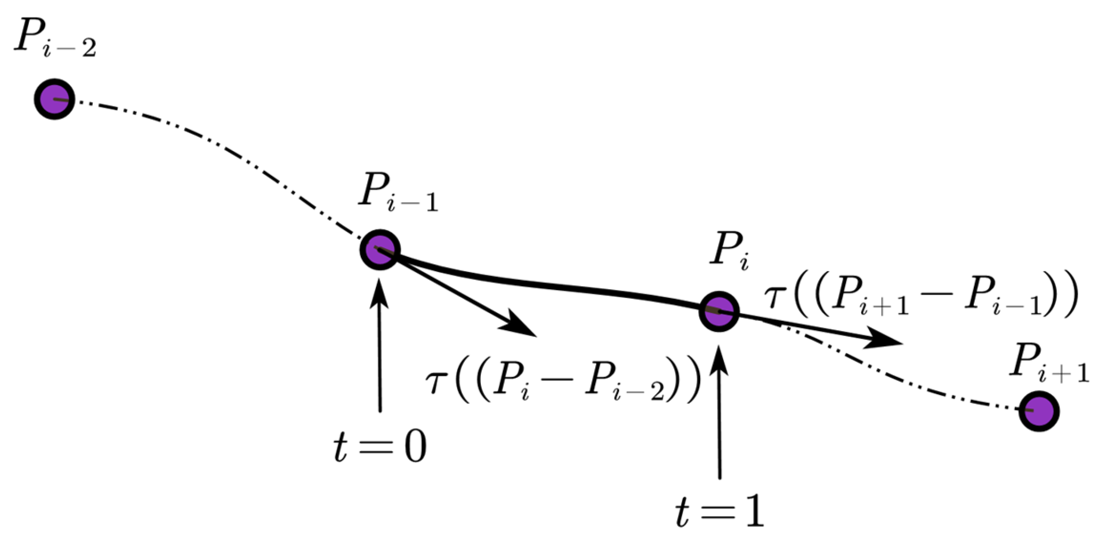
Path smoothing is a key technology in solving space. It aims to achieve a smooth transition of connection points by introducing curves to ensure the continuity of each path segment and the connection points. Since the final path generated by the algorithm in this paper usually has tortuosity and unevenness in a complex map environment, this hurts the path tracking of mobile robots.

Therefore, it is necessary to smooth the generated path to maintain the original path shape more accurately. This paper adopts the Catmull–Rom spline curve to smooth the path, which can effectively improve path continuity and trackability.Specifically as shown in Figure 1.

The specific formula is as follows:

$$M_t=\left[\begin{array}{c}-\mathsf{\tau }+2\mathsf{\tau }{t}^2-\mathsf{\tau }{t}^3\\ 1+(\mathsf{\tau }-3)t^2+(2-\mathsf{\tau })t^3\\ t+(3-2\mathsf{\tau })t^2+(\mathsf{\tau }-2)t^3\\ -\mathsf{\tau }{t}^2+\mathsf{\tau }{t}^3\end{array}\right]$$

(20)

By substituting four points of the generated path into the formula in sequence, interpolation calculations between the path points can be carried out, thus achieving curve smoothing. The goal is to smooth the generated path. To maintain the original path shape as much as possible, it is only necessary to make the Catmull–Rom spline curve pass through each path point and construct the corresponding curves by using three adjacent points in turn. The smoothed path has a continuous curvature, which can effectively reduce the problems of jitter and sharp turns of the mobile robot caused by sudden changes in the path curvature. In addition, this smoothing process can accurately restore the original path, thus significantly improving the smoothness of the path.

3.3.2. Path Restoration Optimization

After the robot completes the avoidance maneuver, it must reach the next target point. If the local target point before the avoidance is still selected as the guide after the local obstacle avoidance, it usually leads to path redundancy. By adding a progressive enhanced potential field oriented towards the global path and introducing an attraction function between the robot and each node, the robot can smoothly return to the worldwide path after performing local dynamic obstacle avoidance. The design of the attraction function is as follows:

$${\mathrm{F}}_{\mathrm{aqt}}(q)=k_{aqt}·{({\displaystyle \frac{d(q)}{d_0}})}^{\mathsf{\psi }}·\left[\begin{array}{l}{\cos \theta }_{\mathrm{q}}\\ {\sin \theta }_{\mathrm{q}}\end{array}\right]$$

(21)

Among them, $q$ is the current position of the robot, $d(q)$ is the distance from the current position to the farthest node of the original trajectory within its search range, ${\theta }_{\mathrm{q}}$ is the angle of the path tangent direction, $k_{aqt}$ is the gravitational coefficient, $d_o$ is the diameter of the robot, and $\mathsf{\psi }$ is the nonlinear factor.

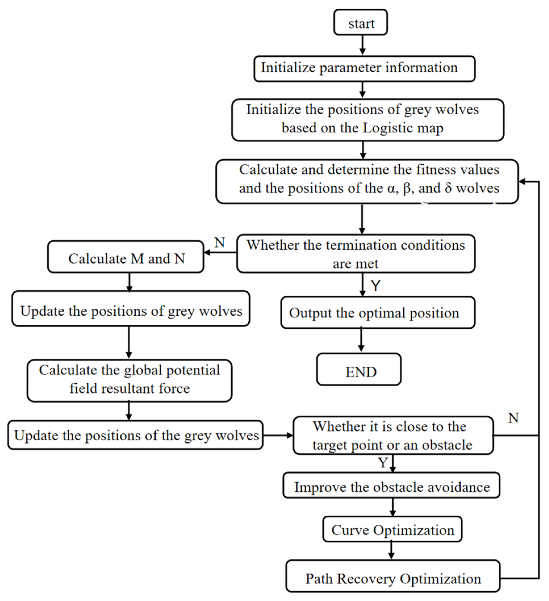
3.4. Overall Algorithm Flow

As shown above, in a large-scale warehouse environment with numerous obstacles, the multi-mobile robot system has difficulties in quickly and accurately finding the optimal trajectory between the starting point and the target point. Moreover, the generated trajectory is prone to falling into a local optimum, leading to the failure of path planning. The LAPGWO algorithm proposed in this paper can effectively realize path planning in a large-scale warehouse environment. The population is evenly distributed during initialization by introducing the logistic chaotic mapping, avoiding omitting the optimal solution. The artificial potential field method is introduced to further accelerate the algorithm’s search efficiency. In response to the problem of an unreachable target, a repulsive force correction term function is proposed to adjust the sensitivity of the target guidance to the change of distance and solve the problem of target unreachability. An independent environmental repulsive field and a robot repulsive field are established for each robot. Dynamic obstacle avoidance can be achieved when encountering dynamic obstacles or coming too close to other robots. The overall algorithm flowchart is shown in Figure 2.

4. Results

In this section, simulation experiments will be carried out in a warehouse environment to verify the feasibility and advancement of the proposed algorithm. All the codes in this paper are written in MATLAB 2021a. All the experiments are run on a Lenovo desktop computer equipped with a Core i5-12500H CPU with a frequency of 2.5 GHz and 16 GB of memory. The parameter settings of the algorithm are shown in

Table 1. Algorithm parameter setting.

Parameters	Setting Values
Population size	60
Search dimension $n$	30
Maximum number of iterations $T$	600
Chaotic interval $\mathsf{\mu }$	3.57–4
Perturbation intensity coefficient $\mathsf{\eta }$	0.1–0.3
Gravitational gain coefficient $\mathsf{\zeta }$	0.5–2
Correction coefficient $\mathsf{\gamma }$	0.1–0.5
Repulsive force gain coefficient $\mathsf{\rho }(t)$	20–40
Adaptive potential field weight $\mathsf{\lambda }$	0.35
Nonlinear factor $\mathsf{\psi }$	0.6
Influence range of obstacles $d_o$	2–3 m
Safety distance threshold between robots $d_s$	1.5 m

. Many preliminary experimental tests have been carried out to obtain a reasonable interval range regarding the values of key parameters, such as the chaotic intensity $\mathsf{\mu }$, the repulsive force gain coefficient $\mathsf{\rho }(\mathrm{t})$, and the disturbance intensity coefficient $\mathsf{\eta }$. The selection of specific optimal parameters will be explained in the subsequent content.

In the simulation experiments of this section, the advancement of the algorithm proposed in this paper is mainly verified. The core objective is conducting a horizontal comparative analysis by comparing it with efficient multi-agent path planning algorithms. The comparative algorithms are the grey wolf optimizer (GWO) algorithm, and the LM-GWO algorithm proposed in reference [26], the CWSO algorithm proposed in reference [28], and the DSA-EGA algorithm proposed in reference [31]. Thirty simulation tests are carried out, and each algorithm’s average path length, running time, and standard deviation are recorded. Furthermore, whether the algorithm in this paper can generate an approximately optimal path planning for the multi-agent system under a single time window constraint is examined.

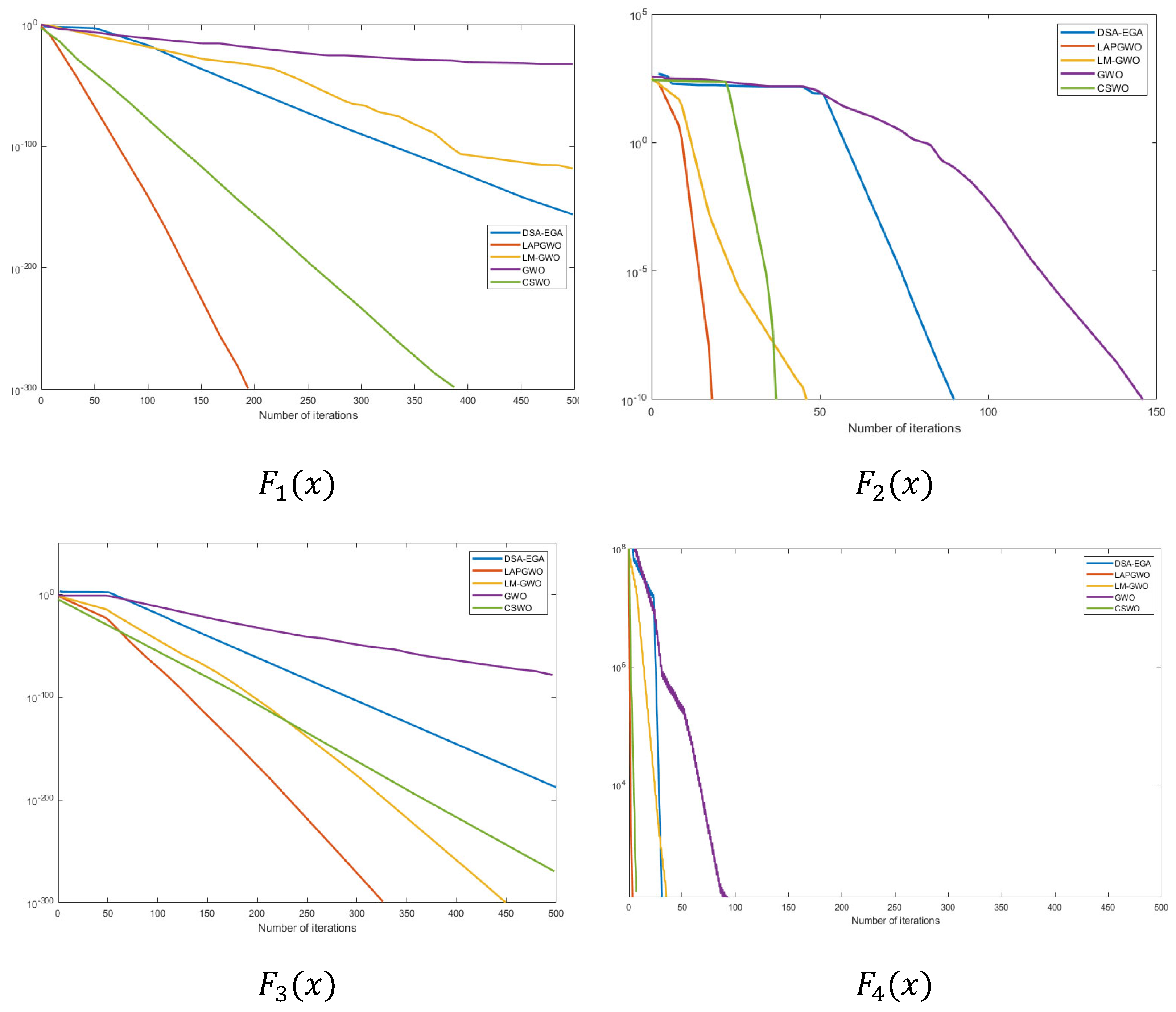
4.1. Comparison of Convergence Curves

Four standard test functions are selected in the experiment, and the detailed information is shown in

Table 2. Standard test function.

Standard Test Function	Dimension	Search	Minimum
$F_1(x)={\displaystyle \sum _{i-1}^d}{({\displaystyle \sum _j^i}{x}_j)}^2$	30	[−100, 100]	0
$F_2(x)={\displaystyle \sum _{i-1}^d}{[100{({x_{i+1}-x}_i^2)}^2+(x_i-1)}^2]$	30	[−30, 30]	0
$F_3(x)={\displaystyle \sum _{i-1}^d}[x_i^2-10\cos (2\mathsf{\pi }{x}_i)+10]$	30	[−5.12, 5.12]	0
$F_4(x)={\displaystyle \sum _{i-1}^d}|x_i\sin (x_i)+0.1x_i|$	30	[−10, 10]	0

. Among them, the unimodal function is $F_1~F_2$, which is used to test the local search ability of the algorithm; the multimodal function is $F_3~F_4$, which is used to test the algorithm’s convergence and global search ability.

The convergence curves of the four algorithms are shown in Figure 2.

As can be seen from

Table 3. Performance comparison.

Function	GWO		LM-GWO		DSA-EGA		LAPGWO		CWSO
	Average Value	Standard Deviation	Average Value	Standard Deviation	Average Value	Standard Deviation	Average Value	Standard Deviation	Average Value	Standard Deviation
$F_1(x)$	6.45 × 10−3	7.123-04	9.47 × 10−9	2.65 × 10−10	3.354 × 107	3.151 × 101	0	0	−1.46 × 10−13	1.22 × 10−7
$F_2(x)$	2.97 × 10	2.86 × 10	2.68 × 10	2.63 × 10	2.91 × 10	2.86 × 10	2.59 × 10	2.51 × 10	0.000197	0
$F_3(x)$	2.80	4.10	0	0	0	0	0	0	0	0
$F_4(x)$	4.29 × ${10}^{-4}$	5.89 × ${10}^{-4}$	1.29 × ${10}^{-271}$	0	3.72 × ${10}^{-4}$	0	0	0	8.83 × ${10}^{-16}$	0

, compared with the other four algorithms, the LAPGWO algorithm obtains an ideal average value, which indicates that the LAPGWO algorithm has better optimization performance; at the same time, the obtained standard deviations are all relatively small, indicating that the improved algorithm has good stability and enhanced local search ability. The LAPGWO algorithm successfully reaches its theoretical optimal value, that is, 0, in the tests of functions [list the functions here if there are specific ones]. This shows that, compared with other algorithms, the average value obtained by the LAPGWO algorithm in the test functions is the best, reflecting that the LAPGWO algorithm has stronger convergence, higher optimal accuracy, and greater stability.

From the convergence curves in Figure 3, it can be seen that, compared with the other four algorithms, the convergence curve of the LAPGWO algorithm shows a rapid decline in the early stage of the search, indicating that the strategy of using the logistic chaotic map to initialize the population can effectively improve the convergence rate in the initial stage of algorithm iteration; in the middle and late stages of the search, the LAPGWO algorithm can more accurately lock the global optimal solution. From the F1 curve, the LAPGWO algorithm can maintain a relatively fast convergence speed and exhibits stronger local exploitation ability. From the F4 curve, the LAPGWO algorithm can effectively avoid local convergence and stagnation phenomena.

4.2. Path Simulation Comparison

4.2.1. Path Recovery

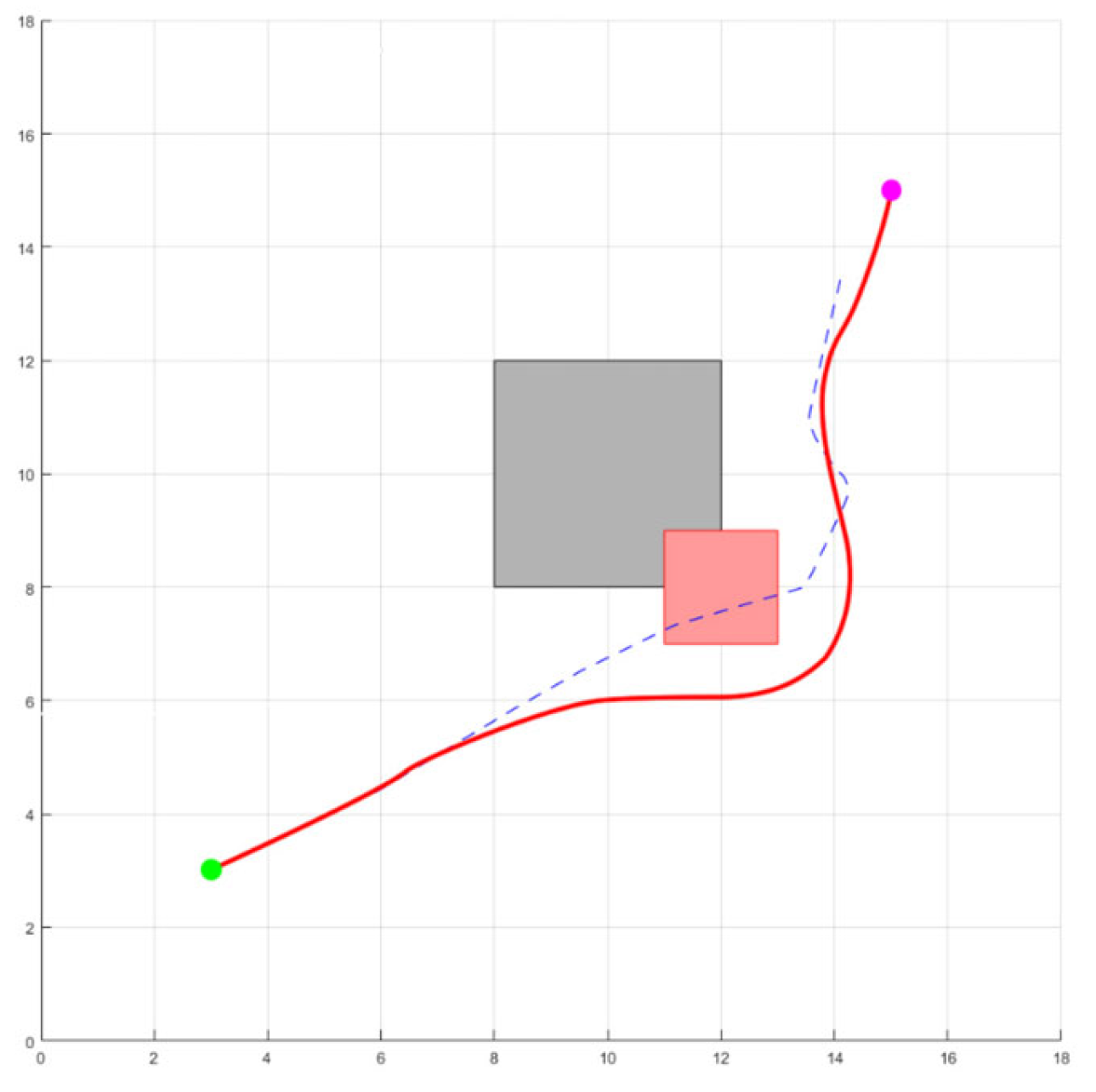
Quickly returning to the original preset trajectory after obstacle avoidance is the key to improving efficiency. As shown in Figure 4, it is a simulation schematic diagram to verify the path restoration method proposed in this paper.

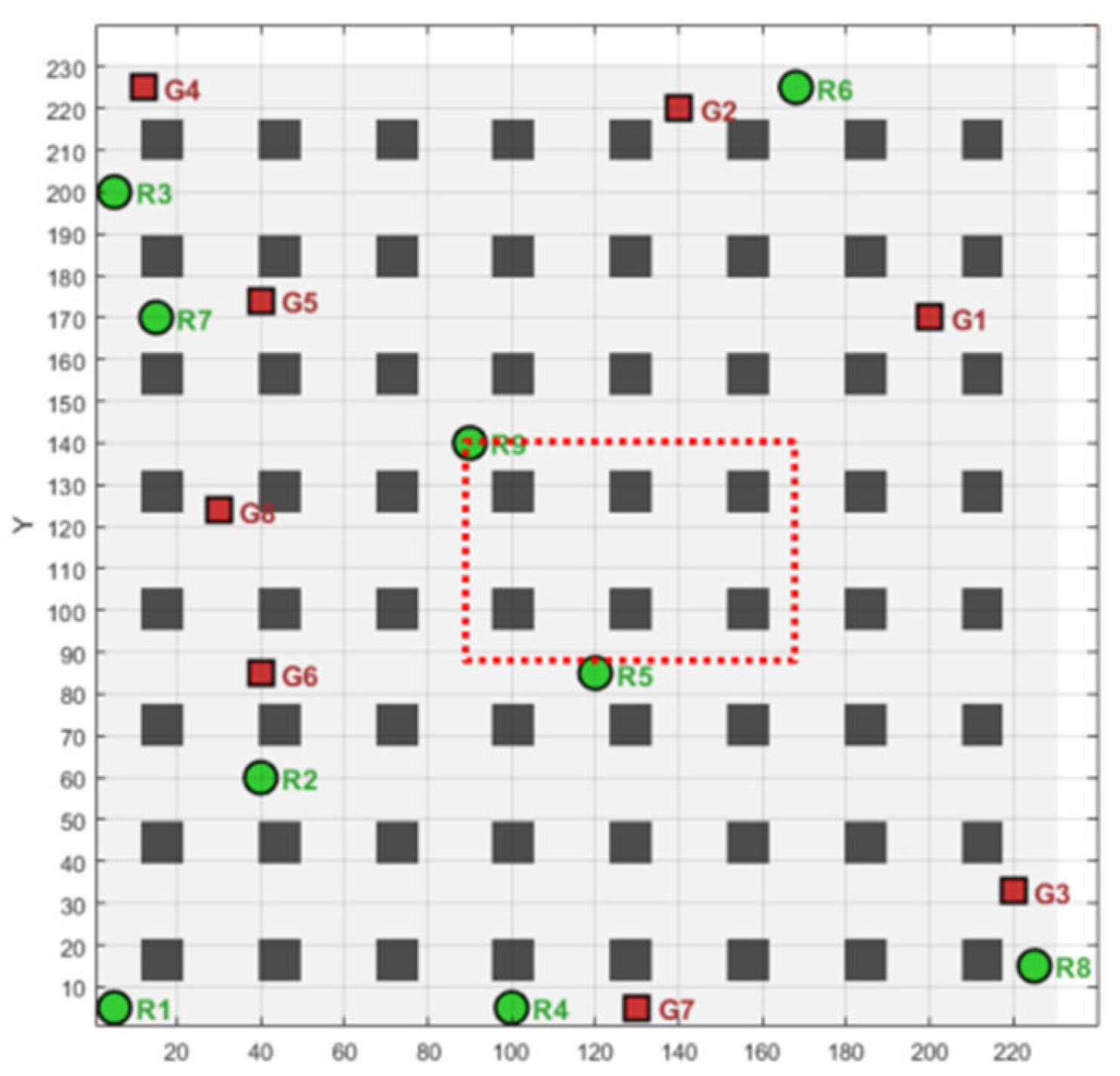
The gray squares represent static obstacles, the red squares represent dynamic obstacles, the blue trajectory is the original path trajectory, and the red trajectory is the optimized trajectory. As can be seen from the figure, when encountering dynamic obstacles, the local artificial potential field method starts to operate for dynamic obstacle avoidance. After the obstacle avoidance is completed, it can quickly and smoothly return to the original preset trajectory, proving the effectiveness of the method proposed in this paper.

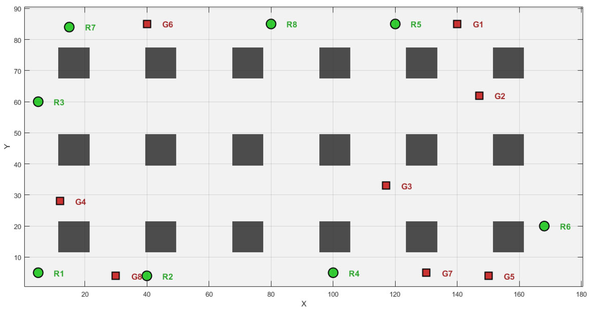
This section will conduct the simulation comparison and verification in three test scenarios to further verify the optimization performance of the LAPGWO algorithm in solving the path planning problem of multiple mobile robots in various environments. The complexity of the obstacles in the three scenarios varies to comprehensively evaluate the generalization ability of the LAPGWO algorithm proposed in this paper and its ability to adapt to the different requirements of the number of obstacles. The three scenarios are as follows: First, there is a simple warehouse environment with a width of 18 m and a length of 9 m. The number of robots is eight, and there are 18 obstacles. The specific scenario is shown in Figure 5. Second, there is a complex warehouse environment with a side length of 23 m. The number of robots is eight, and the number of obstacles is 64. Among them, the green circles represent the initial positions of the robots, and the red squares represent the positions of the target points. The specific scenario is shown in [the corresponding figure]. Finally, there is a non-warehouse environment with a side length of 50 m. The number of robots is eight, and the number of obstacles is 23. A distributed structure is adopted for control. However, considering the computing power of each robot, a unified calculation will be carried out on a single computer. After the calculation, the results will be transmitted to each robot to achieve the effect of distributed control.

4.2.2. Simple Scenario

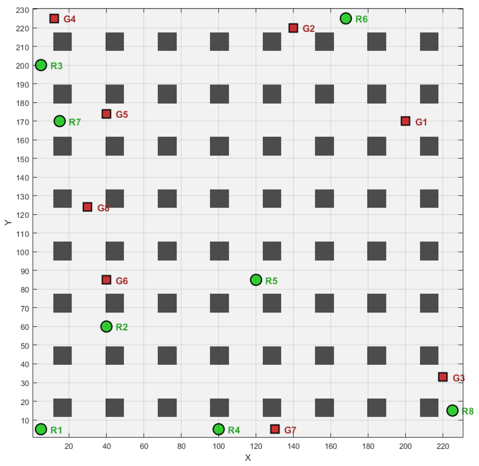
As shown in Figure 5, the rectangular warehouse environment is established. The robots’ initial and target positions are mainly distributed on the area’s periphery. The green circles represent the initial positions, and the red squares represent the target positions.

4.2.3. Determination of Key Parameters

The value range of the chaotic interval determines whether the algorithm can have a strong global search ability in the early stage and focus the search later to improve the search accuracy. The value of the repulsion gain coefficient determines whether it can ensure that appropriate repulsion can be provided for the robot in different scenarios, thus guaranteeing the safety and efficiency of the movement. The perturbation intensity coefficient ensures the algorithm can avoid excessive perturbation, guide the algorithm to jump out of the local optimum, and find the global optimum solution. This paper’s selection of parameters is mainly based on a large amount of experimental data.

To verify the influence of the above key parameters on searchability, this paper will first elaborate on why the range of each parameter is selected and then use the central composite design (CCD) method to find the optimal combination of each parameter.

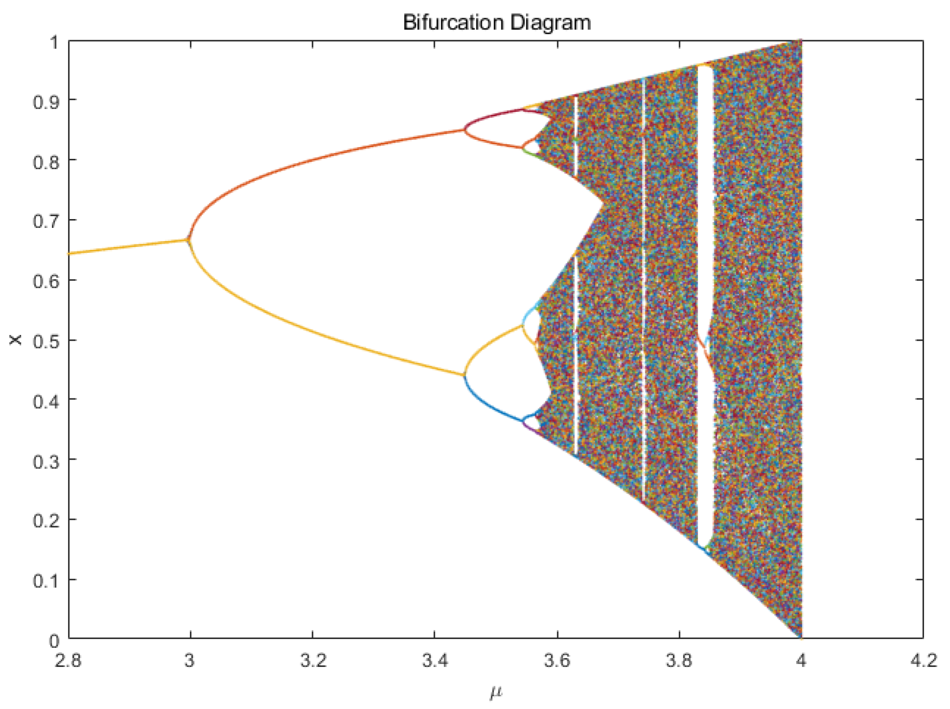
The chaotic interval of the grey wolf population is improved by adding the logistic chaotic mapping. However, the range of the chaotic interval is not the larger, the better. Because for the logistic mapping equation $X_{n+1}=\mathsf{\mu }{X}_n(1-X_n)$, when $\mathsf{\mu }\in (3.57-4)$, the system is in the chaotic region, and the Lyapunov exponent > 0. The system enters the divergence region when $\mathsf{\mu }$ > 4. The chaotic interval diagram is shown in Figure 6.

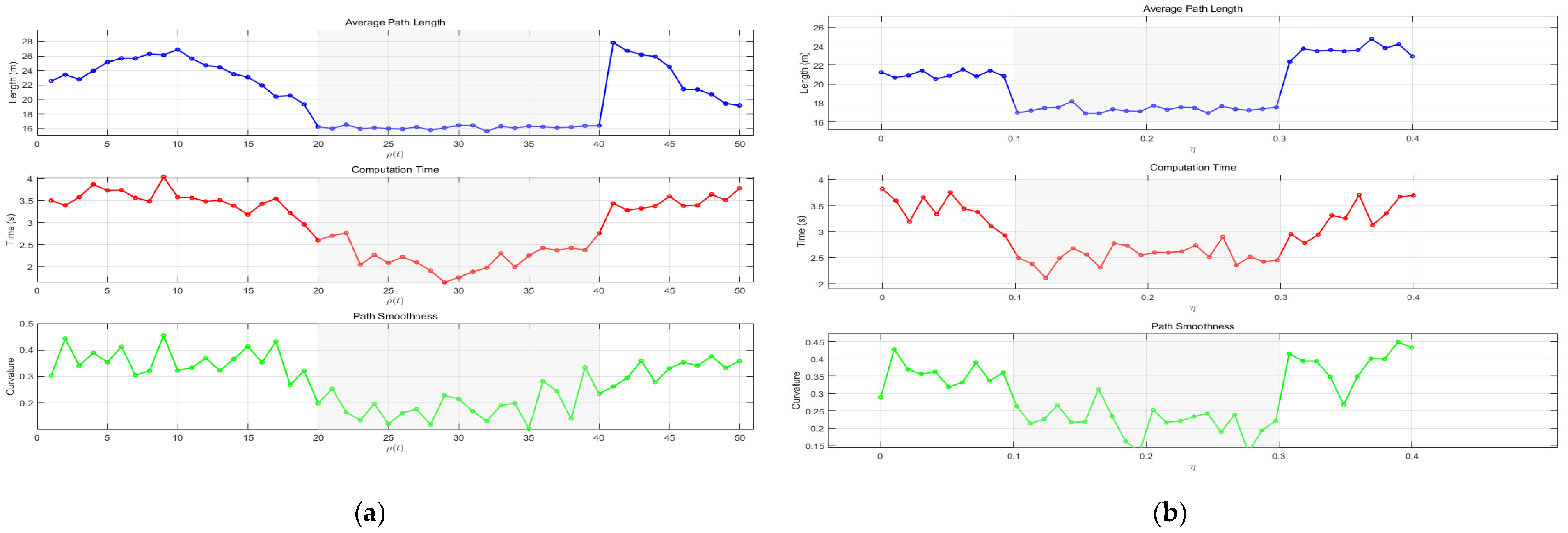
The selection of the ranges of the gain coefficient $\mathsf{\rho }(t)$ and the perturbation intensity coefficient $\mathsf{\eta }$ is shown in Figure 7a,b.

Through a large amount of experimental data, the approximate parameter interval range has been obtained. However, considering the need to find the optimal parameter combination, this paper will use the central composite design (CCD) method to find the optimal parameters, and the results are shown in

Table 4. Test results of key parameters.

Experimental Number	$\mathsf{\mu }$	$\mathsf{\rho }(\mathit{t})$	$\mathsf{\eta }$	Type	Path Length	Computation Time	Path Smoothness
1	3.60	20	0.10	Cubic Point	17.10	3.41	0.24
2	3.60	35	0.27	Cubic Point	16.44	2.42	0.16
3	3.60	40	0.30	Cubic Point	17.57	3.27	0.25
4	3.76	20	0.27	Cubic Point	17.47	3.25	0.23
5	3.76	35	0.30	Cubic Point	17.18	3.11	0.21
6	3.76	40	0.10	Cubic Point	17.21	3.52	0.26
7	3.92	20	0.30	Cubic Point	16.46	3.21	0.22
8	3.92	35	0.10	Cubic Point	16.92	3.16	0.23
9	3.92	40	0.27	Cubic Point	16.21	2.74	0.13
10	3.57	35	0.27	Star Point (Low)	17.29	3.11	0.19
11	4.00	35	0.27	Star Point (High)	16.43	2.668	0.13
12	3.92	20	0.27	Star Point (Low)	17.12	2.752	0.13
13	3.92	40	0.27	Star Point (High)	16.49	2.518	0.12
14	3.92	35	0.10	Star Point (Low)	16.49	2.661	0.17
15	3.92	35	0.30	Star Point (High)	16.44	2.638	0.14
16	3.92	35	0.27	Central Point	16.24	2.514	0.12
17	3.90	34	0.26	Central Point	16.27	2.551	0.13
18	3.94	36	0.28	Central Point	16.33	2.539	0.12

.

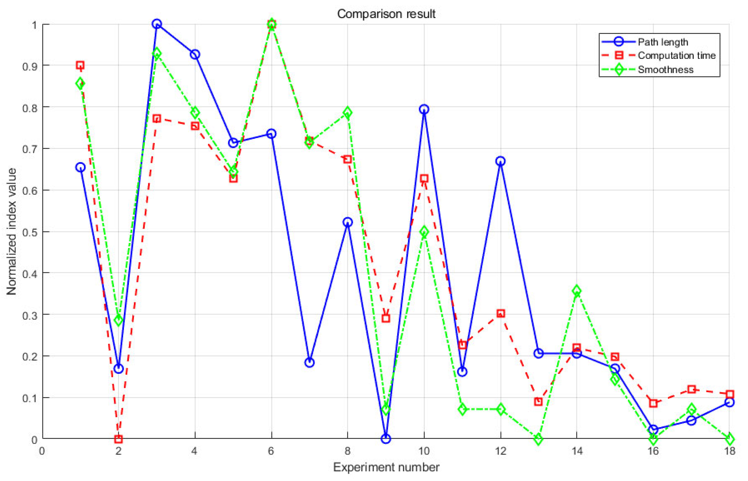
This paper will adopt the method of controlling variables. Under two scenarios and with other variables remaining unchanged, different values will be successively selected for the three parameters to determine the optimal value of each parameter. The specific results are shown in Table 4. For the convenience of result comparison, this paper will normalize the three evaluation indicators of $\mathsf{\mu }$, $\mathsf{\rho }(\mathrm{t})$, and $\mathsf{\eta }$ and present the results in Figure 5. According to the results, the combination of optimal parameters will be determined.

The abscissa of Figure 8 is the experimental number, and each experimental label corresponds to a set of parameter combinations. The blue solid line represents the path length, the red dashed line represents the computation time, and the green dashed line represents the path smoothness. According to the data in the CCD table and Figure 8, different parameter values impact the algorithm’s performance differently. The combination with the experimental number 16 has relatively low values regarding path length, computation time, and path smoothness and is, thus, determined as the optimal parameter combination. Through testing, the following optimal parameter values are obtained: $\mathsf{\mu }$ = 3.92, $\mathsf{\rho }(t)$ = 35, and $\mathsf{\eta }$ = 0.27.

4.2.4. Verification and Analysis of Results in the Rectangular Scenario

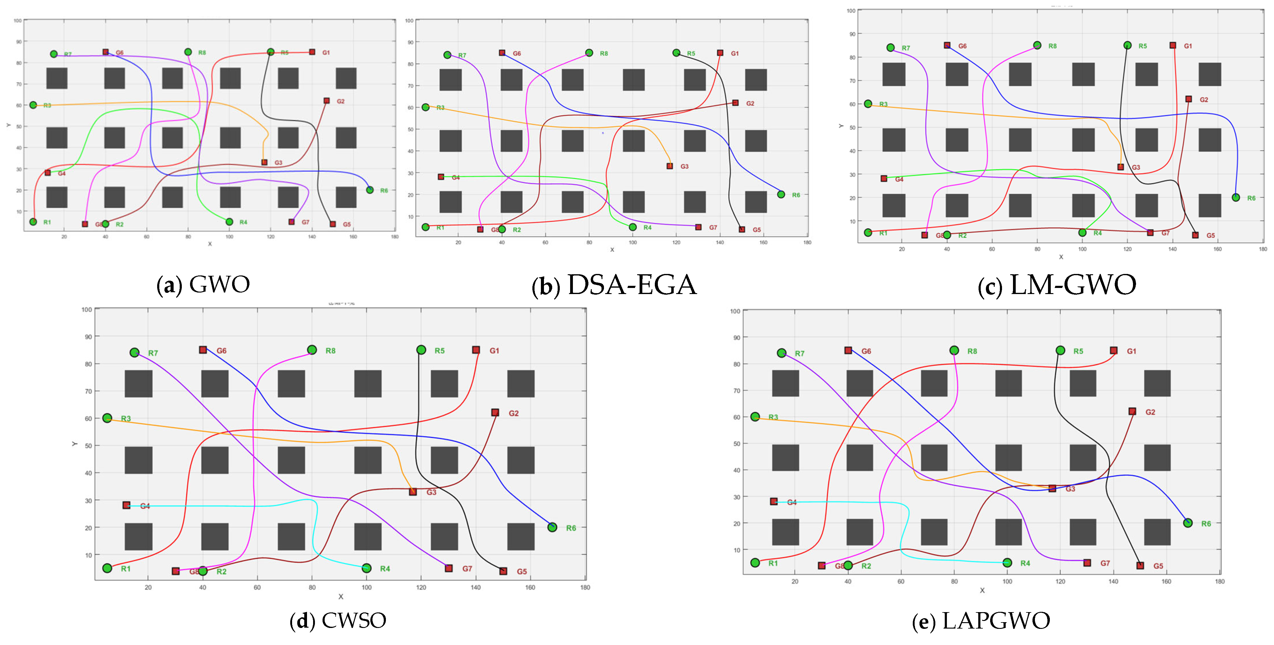
To verify the comprehensive performance of the method proposed in a warehouse environment, the process will be compared and verified with the improved algorithm and the GWO, DSA-EGA, LM-GWO, and CWSO algorithms. The performance of the three algorithms will be evaluated by indicators, such as path length, planning time, success rate, and collision rate, respectively, as shown in Figure 9a–e.

As can be seen from Figure 9 and

Table 5. Results of the simple scenario.

Evaluation Indicators	GWO	DSA-EGA	LM-GWO	LAPGWO	CWSO
Average Path Length (m)	18.14	17.36	17.51	16.24	17.12
Single-Planning Time (s)	3.161	2.749	2.863	2.514	2.681
Path Smoothness (Curvature)	0.47	0.19	0.23	0.12	0.17
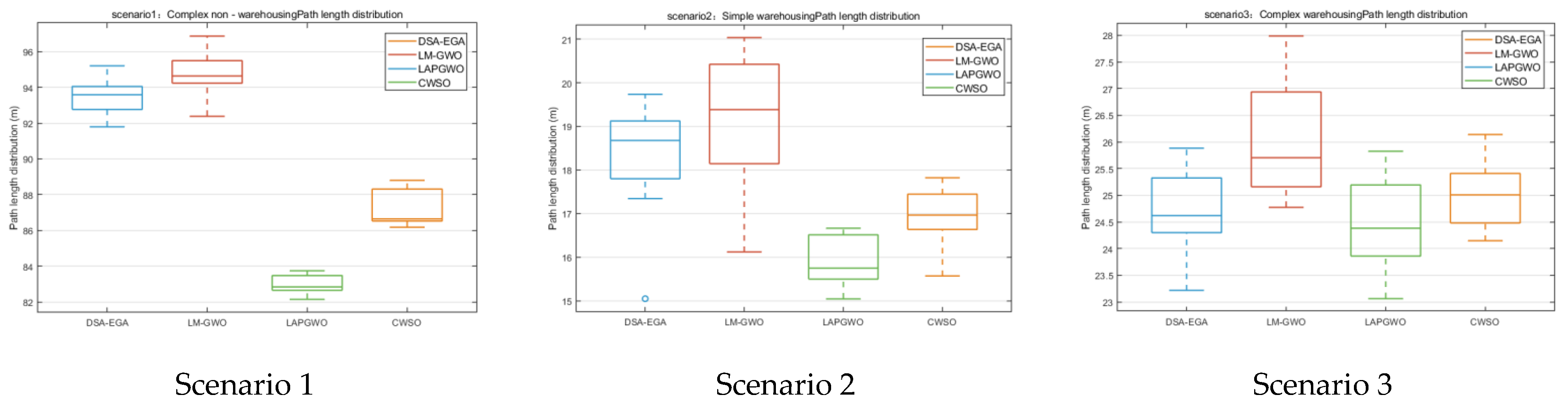
Average Number of Iterations	307	53	81	22	46

, the paths planned by the LAPGWO algorithm have significantly fewer turning points, are smoother, have the shortest average path length, and maintain a certain safe distance from obstacles. The average computation time of the LAPGWO algorithm is improved by 9.1%, 12.3%, and 6.2% compared with the DSA-EGA algorithm, the LM-GWO algorithm, and the CSWO algorithm, respectively. Path smoothness increased by 36.6%, 47.8%, and 29.4%, respectively. The search time, the number of iterations, and the path length of the method proposed in this paper are all superior to those of the DSA-EGA algorithm, the LM-GWO algorithm, and the CSWO and DSA-EGA algorithms. This highlights the advantages of the algorithm in this paper in a simple warehouse environment.

4.2.5. Complex Scenario

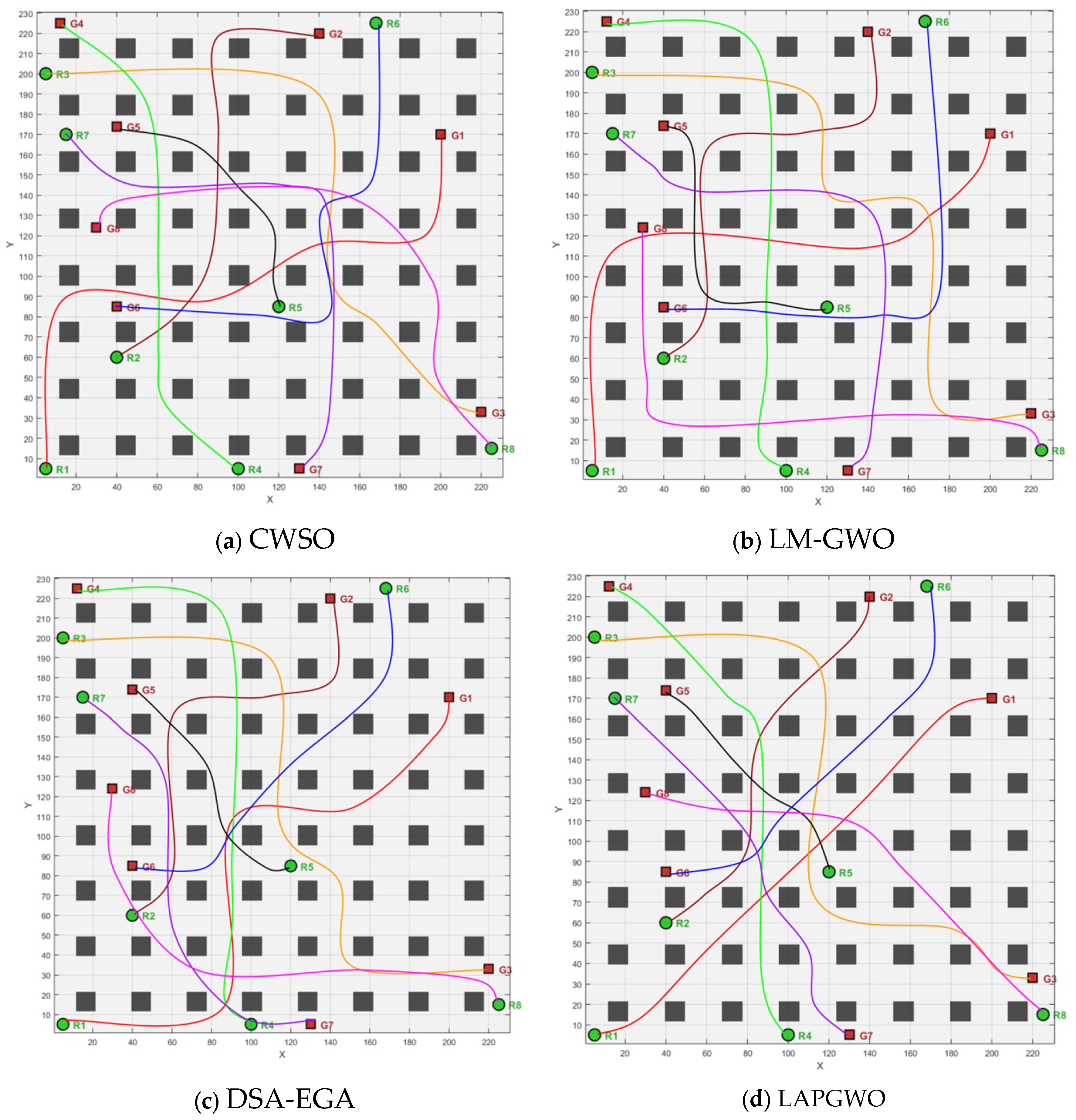
As shown in Figure 10, a complex warehouse environment is established, and the positions of the robot’s initial and target points are randomly generated. The comparative algorithms are DSA-EGA, LM-GWO, LAPGWO, and CWSO. The evaluation indicators are the average path length, planning time, path smoothness, and average number of iterations.

In order to reduce the influence of errors, this paper conducts 100 simulation results, respectively, records the data, and takes the average value as the final index. One of the simulation results is selected for display. The test results are shown in Figure 11 and

Table 6. Results of the performance comparison.

Evaluation Indicators	DSA-EGA	LM-GWO	LAPGWO	CWSO
Average Path Length (m)	25.32	25.81	24.13	25.17
Single-Planning Time (s)	3.417	3.524	3.191	3.208
Path Smoothness (Curvature)	0.24	0.29	0.13	0.16
Average Number of Iterations	62	94	31	61

.

As can be seen from Figure 11 and Table 6, the paths planned by the LAPGWO algorithm have significantly fewer turning points, are smoother, have the shortest average path length, and maintain a certain safe distance from obstacles. The average computation time of the LAPGWO algorithm is improved by 8.3%, 10.5%, and 4.2%, respectively, compared with the DSA-EGA algorithm, the LM-GWO algorithm, and the CSWO algorithm. Path smoothness increased by 37.2%, 55.1%, and 18%, respectively. The search time, the number of iterations, and the path length of the method proposed in this paper are all superior to those of other algorithms.

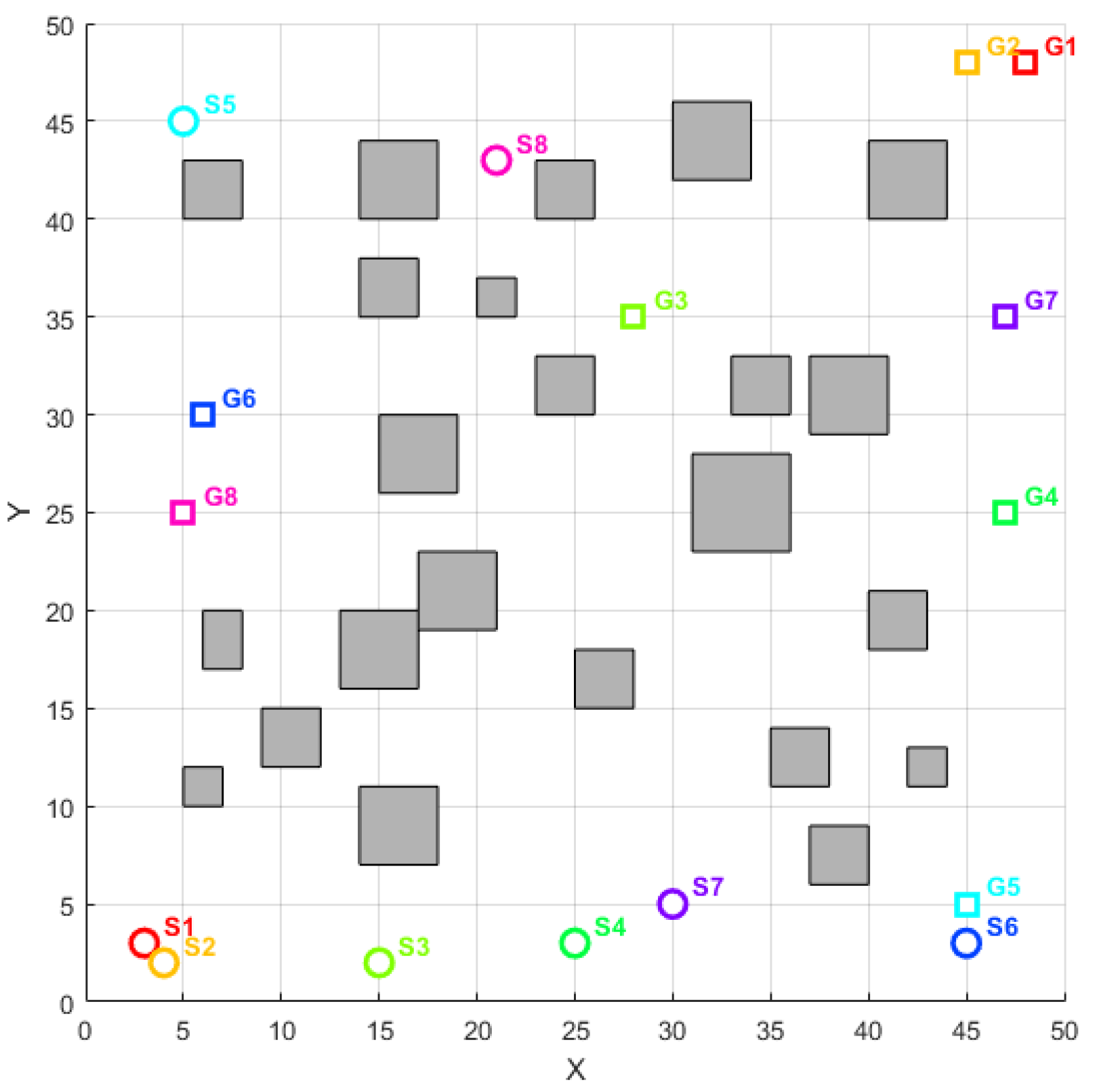
4.2.6. Complex Non-Warehouse Environment

In the warehouse environment, the LAPGWO algorithm exhibits excellent performance. To further verify the adaptability of the LAPGWO algorithm, this paper will continue to conduct tests in complex non-warehouse environments. The comparative algorithms for the test are the DSA-EGA algorithm, the LM-GWO algorithm, and the CWSO algorithm. The map environment is shown in Figure 12.

The positions of the obstacles, the initial point, and the robot’s target point are randomly assigned. The four algorithms’ performance is evaluated by the path length, planning time, path smoothness, and average number of iterations, as shown in Figure 13a–d.

As can be seen from Figure 13 and

Table 7. Comparison of algorithm performance in complex non-warehouse environments.

Evaluation Indicators	DSA-EGA	LM-GWO	LAPGWO	CWSO
Average Path Length (m)	93.12	94.33	82.45	86.81
Average Planning Time (s)	3.247	3.482	2.612	2.871
Path Smoothness (Curvature)	0.32	0.34	0.23	0.29
Average Number of Iterations	91	99	37	84

, the LAPGWO algorithm can still plan an optimal path in a complex non-warehouse environment. The planned path has few turning points, is relatively smooth, and has the shortest length. The algorithm’s performance is superior to that of other comparative algorithms, further highlighting that the algorithm proposed in this paper has strong adaptability in different environments.

4.2.7. Dynamic Complex Scenarios

In practical scenarios, in addition to the robot swarm, there will be other moving obstacles. To further highlight the algorithm’s real-time collision avoidance ability, this paper will add a robot labelled No. 9 as a dynamic obstacle in a complex warehouse environment. The dynamic obstacle will move dynamically within a specified area, and 50 tests will be conducted, with one selected for display. As shown in Figure 14, it is the movement diagram of the dynamic obstacle. The red dashed path is the movement path of the obstacle. The comparative algorithm is the LM-GWO algorithm, and the comparison results are shown in Figure 15. Among them, Figure 15a is the operation result diagram of the LM-GWO algorithm, and Figure 15b is the operation result diagram of the LAPGWO algorithm.The specific experimental data are shown in

Table 8. Comparison of algorithm performance in dynamic areas.

Evaluation Indicators	LM-GWO	LAPGWO
Average Path Length (m)	29.83	25.85
Average Planning Time (s)	4.083	3.378
Path Smoothness (Curvature)	0.43	0.26
Conflict Avoidance Rate	88	96

.

As can be seen from Figure 15, compared with the LM-GWO algorithm, the LAPGWO algorithm proposed in this paper can plan a path that can avoid obstacles in real time when facing the dynamically moving obstacle robot No. 9, with a conflict avoidance rate of 96%, ensuring the safety of the robot’s travel. However, when the LM-GWO algorithm faces the dynamic obstacle No. 9, it will encounter the problem of search failure multiple times and collide with No. 9, with a conflict avoidance rate of 88%, and the generated path is not the optimal path. The comprehensive comparison test results of the algorithms are shown in

Table 9. Comparison of comprehensive performance.

Algorithm	Simple Warehouse			Complex Warehouse			Complex Non-Warehouse			Comprehensive Results
	Path Length	Computation Time	Path Smoothness	Path Length	Computation Time	Path Smoothness	Path Length	Computation Time	Path Smoothness
GWO	18.14	3.161	0.47	\	\	\	\	\	\	\
DSA-EGA	17.36	2.749	0.19	2.532	3.417	0.24	93.12	3.247	0.32	3
LM-GWO	17.51	2.863	0.23	2.581	3.524	0.29	94.33	3.482	0.34	4
CWSO	17.12	2.681	0.17	2.517	3.208	0.16	86.81	2.871	0.29	2
LAPGWO	16.24	2.514	0.12	2.413	3.191	0.13	82.45	2.612	0.23	1

.

In this paper, multiple tests were carried out according to the three scenarios, and an ANOVA significance test was conducted on each algorithm based on the path length information. The test results of the three scenarios are shown in Figure 16. By adding significance verification, it is demonstrated that there are apparent differences between the LAPGWO algorithm and other methods.

From the ANOVA significance test results in Figure 16 and the comprehensive performance comparison results in Table 9, the LAPGWO algorithm proposed in this paper has significantly improved. It ranks first in the comprehensive test results, followed by the CWSO algorithm in second place, the DSA-EGA algorithm in third place, and the LM-GWO algorithm in fourth place.

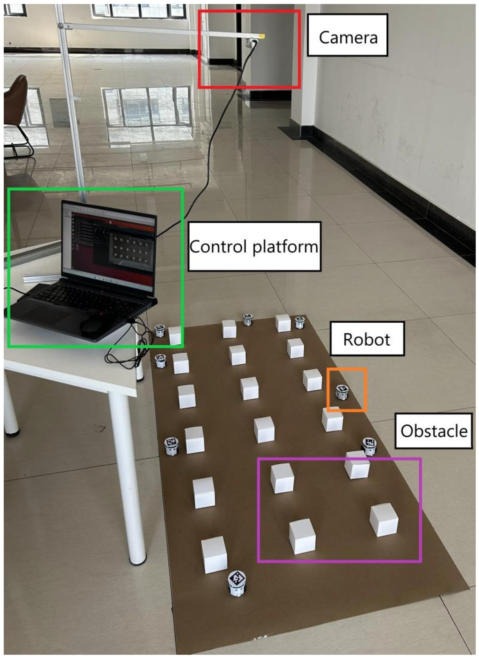
4.3. Physical Experiment Platform

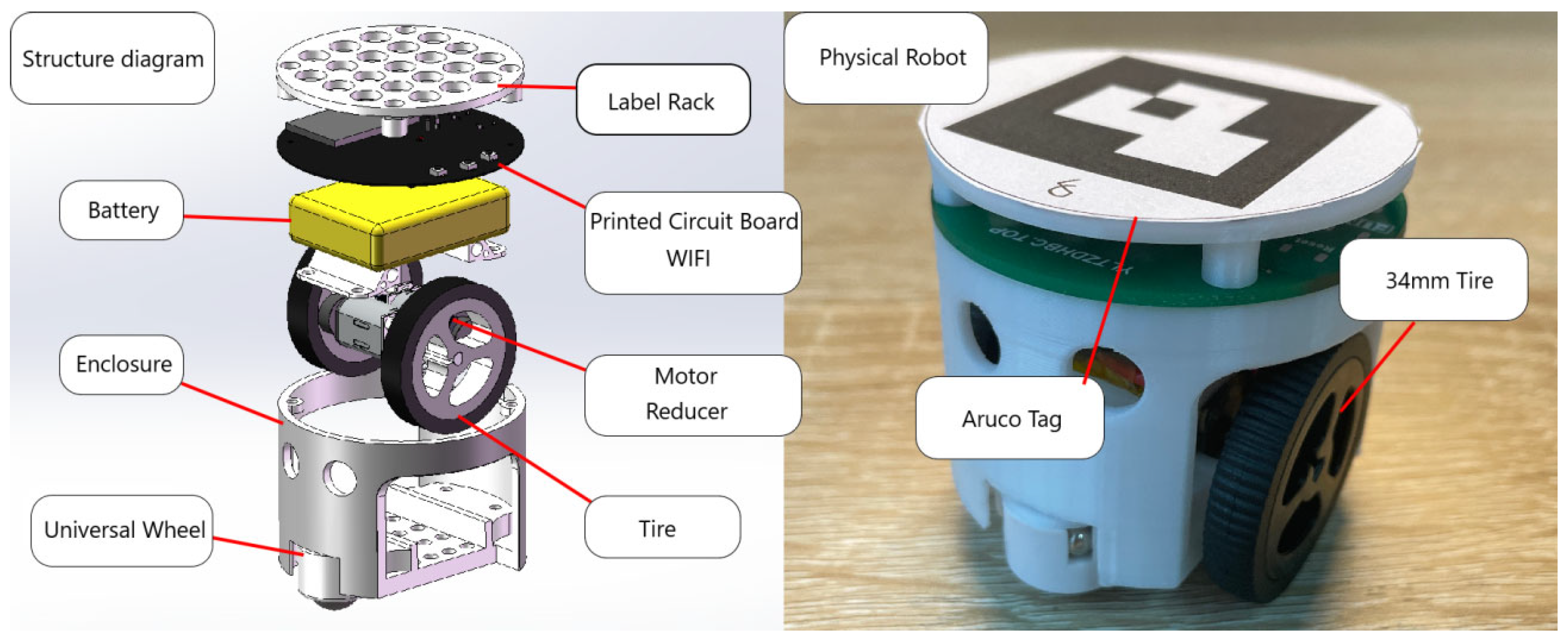
To verify the practical applicability of the method proposed in this paper, a small mobile robot independently built by the research group is used for a physical experiment. The experiment adopts a distributed structure. The main control center calls the global camera to identify the ArUco tags on the top of the mobile robots to obtain their positions, and the position information is fed back to the controllers of each mobile robot in real time. The robots will receive the transmitted position and global map information in real time. The robots share their pose information, autonomously calculate the generated trajectory, and perform obstacle avoidance according to the information. Considering the computing power of the small mobile robots, all data are calculated on the central controller, and the calculation results are transmitted to each small robot to achieve the effect of distributed control.

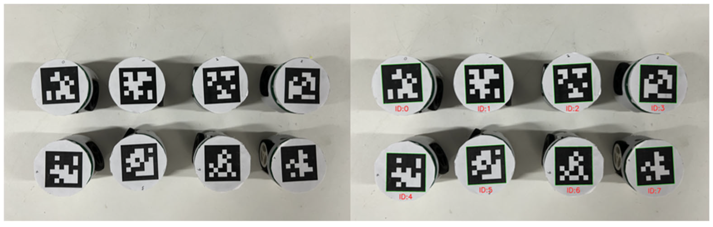
The physical experiment platform mainly includes a central controller, a visual recognition part, and mobile robots. The visual recognition uses the ArUco (augmented reality University of Cordoba) tag technology. The ArUco tag is square, with a black background, and the white rectangle inside stores numerical numbers and other information in a specific encoding. Each robot is pasted with a given ArUco tag in this section’s physical experiment. The camera identifies the ArUco tag on the robot and transmits the information to the control platform. After receiving the information, the control platform processes the information to determine the position information and number information of each robot. The information is displayed visually on the upper computer interface, which is convenient for debugging and data analysis.

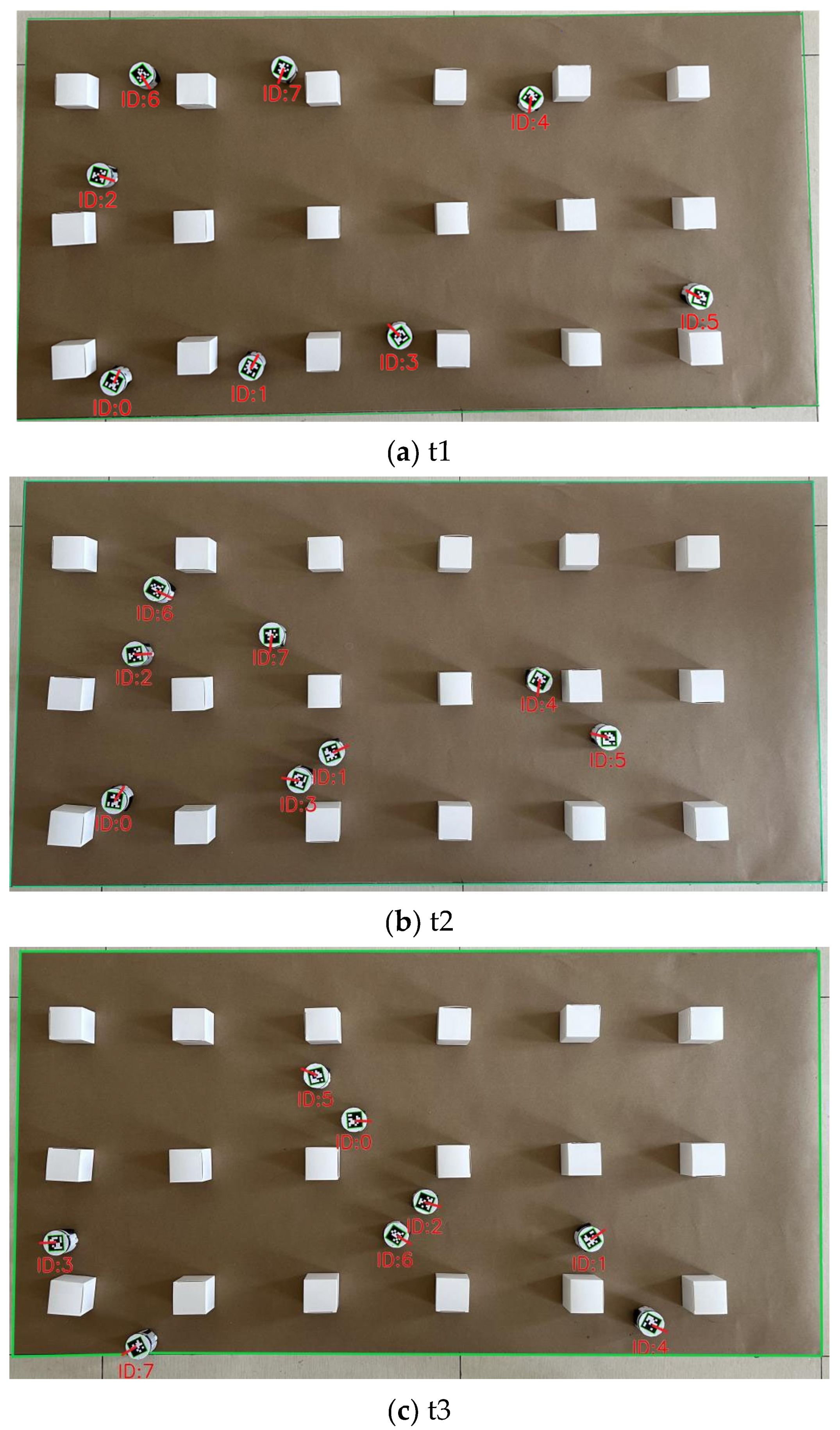
The structural composition diagram of the experimental robot is shown in Figure 17 and Figure 18. Figure 9 shows the pose recognition effect of the experimental robot. The experimental platform is composed of miniCup robots and a central controller, which can effectively identify the pose information of the robots. The upper computer identifies the ArUco tags through the camera to obtain the two-dimensional pose information of each robot. It transmits the real-time pose information of each robot to each robot through the local area network. Due to the computing power problem of the robots, in this section, the central controller will carry out unified processing, plan the path, and output the results to each robot to achieve the effect of distributed control. Due to the limited experimental conditions, the physical experiment environment in this section is verified based on the above simulation experiment. The verification map is shown in Figure 19, which is a physical warehouse environment. The size of the experimental map is simulated and built as 1/100 of the actual simulation environment.

Parchment paper is used as the driving road surface to eliminate the interference of other factors. The road surface is a rectangle with a length of 1.8 m and a width of 0.9 m, and cartons replace the warehouse shelves. The robots are randomly distributed on the map and move autonomously from the starting point to the target point. The robot numbers range from 0 to 7, corresponding to numbers 1 to 8 in the simulation. The respective initial position coordinates are (0.042 m, 0.049 m), (0.418 m, 0.042 m), (0.046 m, 0.591 m), (1.104 m, 0.061 m), (1.197 m, 0.849 m), (1.687 m, 0.218 m), (0.152 m, 0.851 m), and (0.799 m, 0.861 m). The target point coordinates are (1.409 m, 0.848 m), (1.481 m, 0.620 m), (1.178 m, 0.333 m), (0.404 m, 0.861 m), (1.511 m, 0.044 m), (0.418 m, 0.855 m), (1.311 m, 0.052 m), and (0.316 m, 0.040 m) in turn. A camera carries out the data collection of each small robot mounted 2 m above the map, and it is connected to the network through the onboard AP chip to form a local area network with the PC control platform. The mass of the mobile robot is 0.01 kg, the wheelbase is 0.05 m, the distance between the center of mass and the center of the wheel axle can be set as 0.01 m, the preset speed of the mobile robot is set as 0.04 m/s, and the maximum moving speed is 0.2 m/s.

4.4. Analysis of the Results of the Physical Experiment

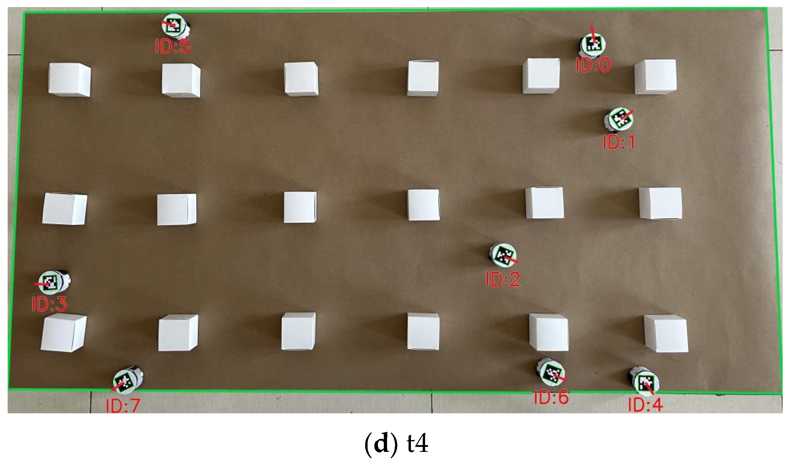
Figure 19 shows the experimental process of the multi-robot system in the warehouse environment using the method proposed in this paper on the physical experiment platform. Among them, a, b, c, and d are the diagrams of four moments during the driving process, respectively.

Figure 20a shows the moment the robot has just started. At this time, the main driving obstacle for the robot is fixed obstacles. Figure 20b,c represents the main obstacle avoidance moments. During this period, the robot must avoid collisions with obstacles, and it is also when various robots converge. The robots also need to avoid other robots on their own. Figure 20d shows the moment the robot autonomously moves towards the target point after the convergence ends until it reaches the given target point. From the actual driving process, it can be seen that the driving trajectory is consistent with the simulation result in Figure 9e. There is no collision with obstacles and other robots during the driving process. The method proposed in this paper shows promising results in practical applications, and it can achieve the goal of not colliding with obstacles and robots during the driving process and smoothly reaching the given target pointAs shown in Figure 20, from a to d are the operation diagrams at the moments of t1, t2, t3, and t4 during the operation.

This paper records the actual driving data of each robot. It compares it with the data of the simulation structure to verify the trajectory tracking error of the method proposed in this paper. The specific measurement table of the trajectory tracking error is shown in

Table 10. Trajectory tracking error measurement table.

Serial Number	Lateral Error	Longitudinal Error	Heading Error	Total Trajectory Error	Maximum Instantaneous Error	RMSE (M)
1	0.18	0.12	2.2	0.21	0.28	0.08
2	0.13	0.09	1.9	0.16	0.23	0.06
3	0.15	0.11	2.5	0.19	0.30	0.09
4	0.16	0.14	2.8	0.21	0.35	0.12
5	0.11	0.08	1.7	0.13	0.2	0.06
6	0.10	0.07	1.5	0.12	0.18	0.04
7	0.09	0.06	1.3	0.11	0.16	0.03
8	0.07	0.05	1.0	0.09	0.12	0.02
Mean value	0.124	0.090	1.863	0.153	0.228	0.063
Standard deviation	0.035	0.028	0.614	0.043	0.084	0.033

.

5. Conclusions

In a complex dynamic warehouse environment, the multi-mobile robot system faces a complex environment, and the GWO algorithm has difficulty quickly and accurately finding an optimal path to the target point, resulting in low efficiency. An improved grey wolf optimization algorithm (LAPGWO) combining the logistic chaotic mapping and the artificial potential field method (APF) is proposed. Based on the logistic chaotic mapping, a uniform chaotic sequence is generated to increase the diversity of the population and improve the search efficiency. At the same time, chaotic disturbances are introduced when updating the positions of grey wolves to avoid premature convergence. Based on the APF, gravitational and repulsive force fields are constructed to promote the movement of grey wolves toward the target point and keep grey wolves away from obstacles, further accelerating the search speed.

Given the dynamic characteristics of the warehouse environment, optimization and improvement are carried out based on the artificial potential field method. A repulsive force field between robots is constructed to avoid collisions between robots. A repulsive force correction term function is built to solve the problem of unreachable targets. The generated path is smoothed using the Cantmull—Rom spline curve to improve path continuity and traceability. A path restoration function is constructed to enable the robot to return to the global path smoothly after obstacle avoidance and reduce path redundancy. The advancement and practical applicability of the method in this paper are further verified through simulation and physical comparison experiments. In contrast, the experiments in this paper are mainly conducted in simulation and relatively ideal environments. When in an actual complex environment, the environment is imperfect, and issues such as sensor noise and communication delays must be considered. When facing other environments, the selection of various parameters still requires a large number of repeated tests to obtain the optimal range. In the follow-up, this paper will conduct the adaptive optimization of the parameters to meet the application requirements of different scenarios.

In addition, the experiments in this paper are mainly carried out in simulations and relatively ideal environments. In an actual complex environment, the environment is not in an ideal state, and many factors must be considered. In the future, we will further optimize the method, seek solutions to possible problems in practical applications, and apply it to the actual workspace.