Article

A Real-Time Green and Lightweight Model for Detection of Liquefied Petroleum Gas Cylinder Surface Defects Based on YOLOv5

by
Burhan Duman
Department of Computer Engineering, Faculty of Technology, Isparta University of Applied Sciences, 32100 Isparta, Turkey
Appl. Sci. 2025, 15(1), 458; https://doi.org/10.3390/app15010458
Submission received: 2 December 2024 / Revised: 25 December 2024 / Accepted: 26 December 2024 / Published: 6 January 2025
(This article belongs to the Section Green Sustainable Science and Technology)

Abstract

:
Industry requires defect detection to ensure the quality and safety of products. In resource-constrained devices, real-time speed, accuracy, and computational efficiency are the most critical requirements for defect detection. This paper presents a novel approach for real-time detection of surface defects on LPG cylinders, utilising an enhanced YOLOv5 architecture referred to as GLDD-YOLOv5. The architecture integrates ghost convolution and ECA blocks to improve feature extraction with less computational overhead in the network’s backbone. It also modifies the P3–P4 head structure to increase detection speed. These changes enable the model to focus more effectively on small and medium-sized defects. Based on comparative analysis with other YOLO models, the proposed method demonstrates superior performance. Compared to the base YOLOv5s model, the proposed method achieved a 4.6% increase in average accuracy, a 44% reduction in computational cost, a 45% decrease in parameter counts, and a 26% reduction in file size. In experimental evaluations on the RTX2080Ti, the model achieved an inference rate of 163.9 FPS with a total carbon footprint of 0.549 × 10⁻³ gCO2e. The proposed technique offers an efficient and robust defect detection model with an eco-friendly solution compatible with edge computing devices.

1. Introduction

Quality control is one of the most important aspects of industrial processes, ensuring that manufactured products will not harm their users. Critical product defects may cause production interruptions, reduce product lifespan, and result in environmental and economic damages. Regular inspections during both the operational and usage phases are necessary to detect defects as early as possible, so appropriate actions can be taken.
Liquefied petroleum gas (LPG) is an environmentally friendly source of energy with wide applications in industrial plants and private households [1]. In recent decades, portable LPG cylinders have been a major source of heat energy in developing countries, particularly in rural areas. After use, LPG cylinders are refilled in industrial plants and returned to the market. It is crucial to identify and scrap surface-defective cylinders before refilling, to maintain quality standards, ensure safety, and uphold the processes for LPG cylinders. The decision to scrap the cylinder is based on the types of defects identified according to the TS EN 1439 standard [2]. These defects are the presence of large and multiple dents on the cylinder body, removal of paint and metallised coating from the cylinder body, and deformations such as multiple intersecting dents, gouges, and cracks that disrupt the visual integrity of the body and show colour changes in shades of grey. Such deformations, which may endanger the structural integrity of the cylinder, may prevent safe use of the cylinder and may require the tube to be scrapped.
Surface defect detection methods can be broadly categorised into traditional and machine learning-based approaches. Traditional defect detection, which existed before artificial intelligence or machine learning techniques, involved a variety of methods such as manual inspection, non-destructive testing (NDT), and image processing. With manual methods, defects on the product surface are usually detected by the eyes and hands of the responsible personnel. The success of detection is a subjective matter that depends entirely on the expertise and attention of the personnel. It is prone to errors caused by human factors such as fatigue and distraction. However, speed is required to keep up with automated systems [3].
NDT methods such as ultrasonic testing, magnetic particle testing, liquid penetrant testing, and radiographic testing are traditional approaches used to detect internal or surface defects without damaging the material. Although effective, these methods can be time-consuming and require skilled personnel, which can limit their scalability and adaptability to automated processes [4]. The detection of surface defects using image processing is a computer-aided method. These techniques include edge detection, histogram analysis, filtering, and morphological operations [5,6,7,8,9]. While they can show good results when there is variation between defect colour and background (texture differences in the background, noise, and lighting conditions) [10], their performance is based on manually prepared feature selection and a priori assumptions.
Manual feature extraction is may not be suitable for all defects, as these can vary in type, shape, size, and morphology [11]. For example, methods such as edge detection, histogram analysis, and texture analysis are often used in manual feature extraction, but they can pose difficulties in detecting complex or seemingly obscure defects and generalising them to various industrial applications. Traditional approaches to machine learning, including Support Vector Machines (SVM) and K-Nearest Neighbours (KNN), are quite sensitive to environmental factors—like illumination, noise level, complex pattern, or surface texture—but generally less stable with regards to handling changes in these conditions. Hence, deep learning methods have been increasingly being applied for defect detection with more robustness [3,5,12].
Deep learning methods have already been successfully applied in various industries, including printed circuit boards [13], transmission line elements [14], steel sheets [15,16], metallic components [17], textile surface defects [18], and wood surfaces [19].
It is especially deep learning methods involving ANNs that can achieve this automatic extraction of intricate patterns and features from data features that is so necessary for industrial defect detection. Among these methods, convolutional neural network (CNN) algorithms have achieved huge successes recently in image-based defect detection by making inferences at multiple layers through multiscale analysis. Such techniques can even catch defects that might be too small for the resolution power of the human naked eye. The CNN algorithms commonly used in defect detection may be broadly divided into two categories: two-stage methods that construct bounding boxes and estimate information regarding defect location and class and one-stage methods that estimate this information directly. Two-stage methods include RCNN [20], Fast-RCNN [21], and Faster-RCNN [22], while popular one-stage methods include the series of SSD [23] and YOLO [24].
Deep learning models with lightweight architectures are preferred for real-time and efficient execution of defect detection tasks with CNN methods on resource-constrained devices. Surface defect detection with lightweight deep learning models focuses on You Only Look Once (YOLO) architecture, which includes state-of-the-art (SOTA) networks. However, ongoing developments in green deep learning aim to further optimise models such as YOLO to reduce energy costs and carbon emissions while maintaining performance [25,26].
Versions such as YOLOv4 [27] and YOLOv5 [28] have gained widespread adoption in real-time applications, offering fast processing times and high detection accuracy. Numerous strategies have been explored in existing studies to enhance the standard architecture of YOLOv5 to achieve the desired application-specific performance in demanding industrial applications, such as detecting surface defects on industrial liquid gas cylinders with complex backgrounds.
These strategies include developing the efficient channel attention (ECA) mechanism for optimising channel-based attention mechanisms and improving the feature extraction capabilities of the networks [29,30,31]. Ghost convolution and other types of lightweight convolutional layers are used to reduce computational overhead and increase network speed [32,33,34].
This study proposes a YOLOv5-based network design aimed at detecting surface defects on LPG cylinders in resource-constrained devices. The basic model is customised to adapt to the characteristics of LPG cylinder surface defects, limited resources, and real-time detection requirements. The YOLOv5s network is designed to reduce model size, parameter count, computational cost, and carbon footprint. The study’s contributions and innovations to the literature are listed below:
  • A new dataset of 2360 LPG cylinder images with defective surfaces is proposed.
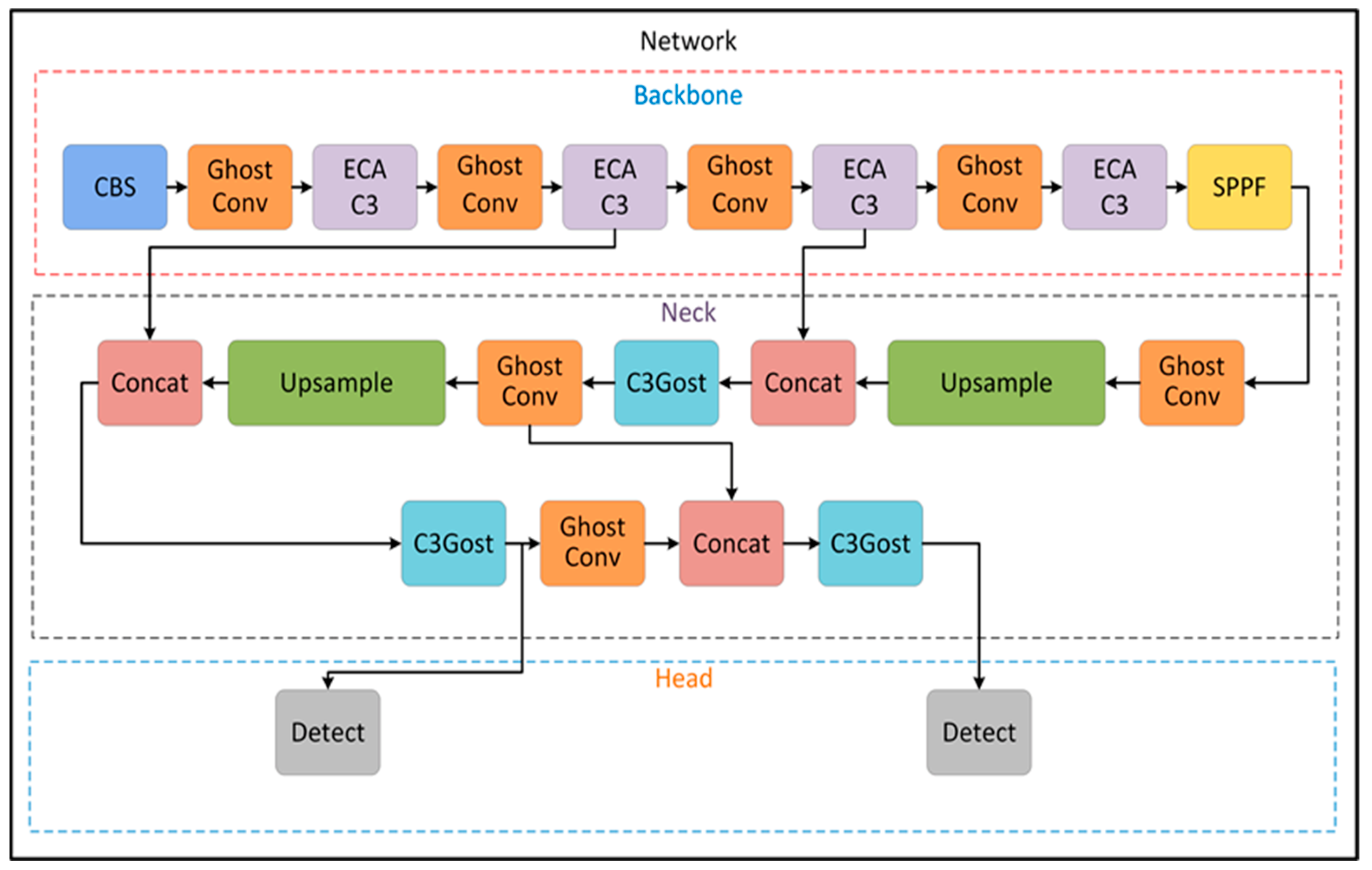
  • To lighten the network, the Ghost module was used both in the backbone and neck sections of YOLOv5. In addition, the C3Ghost module has been added to the neck section, and the P5 head, responsible for detecting large objects, has been removed from the head. In this way, low memory consumption with small model size, reduced computing costs, and fast inference are achieved.
  • In this network, ECA is a channel-based attention mechanism that further optimises this network by enhancing the feature extraction capability to recognise accurate surface defects.
  • The efficacy of the proposed model is validated through comprehensive experimentation on a custom dataset.
The following part of the paper, Section 2, presents studies on defect detection, lightweight networks, and YOLO networks. A detailed explanation of the detection methodology developed in this study is provided in Section 3. Section 4 outlines the dataset, experimental framework, and a comparative evaluation of the obtained results. Section 5 contains the discussion. Finally, Section 6 presents a summary of the overall results of the study.

2. Related Work

2.1. Deep Learning-Based Defect Detection Methods

In the literature, there are CNN-based, transformer-based, and hybrid models where CNN and transformers are integrated into deep learning-based defect detection studies. These studies aim to improve the performance of surface defect detection with different architectural approaches and algorithms. Methods based on both traditional CNN architectures and next-generation approaches have been developed.
A high-accuracy Faster R-CNN algorithm is proposed for fabric surface defect detection, developed for a custom-prepared dataset [35]. For identifying surface defects on railway, a novel network based on Mask R-CNN was developed, achieving an average accuracy of 98.70% [36]. The approach of RAF-SSD combined the attention mechanism along with a multi-feature fusion network and a 12.9% increase in detection rate compared to the traditional deep learning model proposed by Liu and Gao [37].
Transformers, initially popularised in natural language processing, are increasingly gaining attention in computer vision and deep learning-based defect detection due to their key advantages: the attention mechanism, long-range dependency capture, and transfer learning capabilities.
Unlike CNNs operating directly on image pixels, transformers divide an input image into patches of fixed pixel size [38]. Then, they propose a new network architecture, the LSwin Transformer, for the detection of steel surface defects, which showed very promising performance in surface defect detection [39,40]. Another study, named ETDNet, on steel surface defects effectively classified defects of various shapes and sizes [41]. Shang et al. [42] proposed an intelligent surface defect detection method called DATNet, employing a Transformer-based encoder to prevent blade failure and tool wear.
Transformers are general-purpose models that can be adapted for both NLP and computer vision tasks. They have an attentional mechanism that models long-distance dependencies between image regions to dynamically focus on different parts, which makes them effective in variable-sized images or images with irregular structures [43]. However, the self-attention mechanism requires a large computational cost, thus limiting its use on resource-constrained devices, and requires a large dataset for performance reasons. Training and fine-tuning processes, especially the identification of hyperparameters, can be quite challenging [44,45].
CNNs can be successful in extracting low-level features. The natural modelling of locality and translation invariance by CNN fits into image processing [46], making it a great choice for resource-constrained or real-time devices [47]. Quite often, with less data, it is possible to come up with more plausible good performance [48]. In the meantime, local connections are always the primary focus in CNNs, and, to catch dependencies in larger scales, extra layers or more complex architecture are often needed [49]. These two important architectures, when embedded in deep learning defect detection, can revolutionise quality control in an industrial process. Any architecture is thus completely dependent on application and task, since every model may prove most appropriate regarding the considered factors.

2.2. Research on Model Lightweight and Improvement
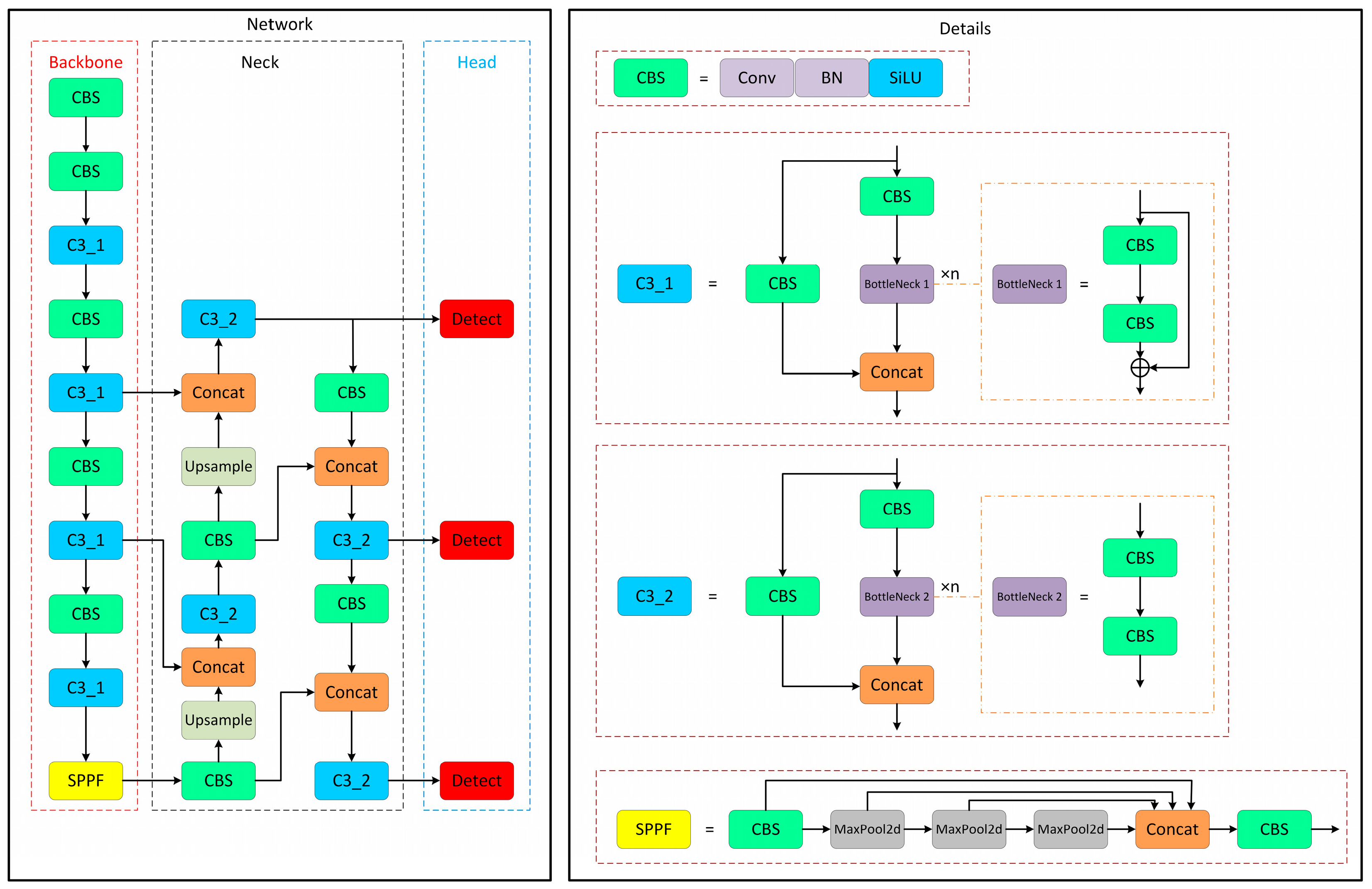
In industrial production and processes, real-time requirements often arise for the detection of objects/defects. Real-time edge devices installed at a production site usually have limited computational capacity, and computational costs make it difficult to deploy large and complex networks [50,51,52]. A model for real-time object detection tasks needs to take into account memory requirements and computational costs and find a balance with detection performance. Therefore, lightweight networks like SqueezeNet [53], MobileNetV1 [54], ShuffleNet [55], and GhostNet [56] have been developed that balance accuracy with speed. In addition, the YOLO series of algorithms have been developed for this purpose.
SqueezeNet puts forth a novel network architecture, designated the fire module, which is designed to achieve satisfactory accuracy with a reduced number of parameters. In its place, a 1 × 1 convolution is employed, and the channel of the 3 × 3 convolution input is reduced. The next stage of the network performs the downsampling. SqueezeNext [57] employs a two-stage compression process to achieve a substantial reduction in the number of channels. The use of a separable 3 × 3 convolution allows for a further reduction in model size.
In the MobileNet series [54,58], the Deep Separable Convolution (DSConv) module has been proposed. By lowering the parameter count, the model is smaller, and the calculations are less complex. It is well-suited to integration into mobile devices. In ShuffleNet, the network is extended by the incorporation of a group convolution module based on DSConv and a channel shuffling.
In ShuffleNetV2 [59], channel splitting is employed in lieu of groupwise convolutions, with the objective of reducing the number of network parameters. This approach is intended to mitigate the potential for a large number of group convolutions and shuffling operations to increase the frequency of memory accesses.
GhostNet proposes a small model architecture, the Ghost module, which is designed to utilise fewer parameters and less computational power. The Ghost module initially generates a feature map via simple convolution and uses various inexpensive linear operations to expand the features and process the spatial information. A significant advantage of GhostNet is that it exhibits excellent feature extraction capability while simultaneously reducing the number of parameters [56].
Although there are no other studies in the literature for LPG cylinder surface defects, similar studies on defect detection with model lightweighting based on YOLO have come to the forefront, with some improvements in each of them.
An improved YOLO-RDP model for metal surface defect detection based on YOLOv7-tiny has been proposed for application in edge devices [60]. In the Backbone part of the model, GSConv and VOV-GSCSP modules are used to optimise RexNet and the neck layer of the network. In addition, a dual-head object detection head called DdyHead is designed, and a pruning method is used. The experimental results showed that 3.7% and 3.5% improvement in mAP values were realised in the NEU-DET and GC10-DET datasets, respectively. In another study, a YOLOv5-based algorithm with three basic (GhostConv, ECAc3, and Decoupled Head) improvements was proposed for real-time detection of defects on the cover surface. The proposed model is named ESD-YOLOv5 [11]. The detection results of the ESD-YOLOv5 model on the study-specific dataset showed a 2.3% improvement in the mAP@50 metric compared to the YOLOv5 baseline model, but a 33% decrease in extraction speed from 137 FPS to 91 FPS. Zhou et al. [61] proposed a new defect detection model (SKS-YOLO) based on YOLOv5s with a simplified kernel and squeeze-excitation module for defect detection on steel plates. The SKS-YOLO model provided 4.4% improvement in accuracy compared to YOLOv5s. While the FPS value of YOLOv5s was 66, it decreased to 55 in SKS-YOLO, resulting in an 18% reduction in extraction speed.
Liu et al. [34] developed an LF-YOLO model based on an EFE module and RMF module for weld defect detection from X-ray images. In the weld defect dataset, the LF-YOLO model achieved an accuracy of 92.9 mAP@50 with a computational load of 4.0 GFLOPs, 7.3 M parameters, and 61.5 FPS, while the basic YOLOv3 (MobileNetv2) model achieved 90.2 mAP@50 accuracy with a computational load of 1.6 GFLOPs, 3.7 M parameters, and 71 FPS. In another study for transmission line defect detection, a model named TLI-YOLOv5 was proposed that incorporates the attention module SimAM into the YOLOv5 network and includes the Wise-IoU loss function [62]. In tests on the UAV transmission line inspection dataset, TLI-YOLOv5 achieved a 2.91% increase in accuracy (mAP50) compared to the original YOLOv5n, with an extraction rate of 76.1 FPS and a model size of 4.15 MB.

2.3. YOLO Networks

The first version of YOLO, YOLOv1 [24], set a new trend in real-time object detection by integrating region proposal and classification into a unified network. Since then, each successive model brought significant improvements in accuracy, efficiency, and real-time performance. YOLOv2 was able to expand detection capabilities into more than 9000 object categories using the Darknet-19 backbone [63]. YOLOv3 introduced Darknet-53 with an FPN architecture to improve small object detection [64]. YOLOv4 [27] and YOLOv5 [28], integrated with the CSPNet [65] backbone and complemented with advanced feature fusion modules such as PANet [66] and SPP [50], pushed this performance even further. YOLOv5 development was done with PyTorch, which made migration to the ONNX and CoreML frameworks quite easy to make it run on iOS devices and mobile apps [67,68].
Recent versions include YOLOv6 [69], YOLOv7 [70], and YOLOv8 [71,72], which have put more emphasis on lightweight architectures, improved backbone designs, and other innovative optimisations such as anchor-free detection and efficient layer aggregation. YOLOv9 [73] introduced GELAN for balancing model lightness, speed, and accuracy, while YOLOv10 [74] integrated dual-label assignment and rank-guided block design for enhanced efficiency [75]. The most recent YOLOv11 model, released in 2024, emphasizes reduced parameters and adaptability for both cloud and edge deployments, showcasing continued advancements in real-time object detection [71].

YOLOv5s Architecture
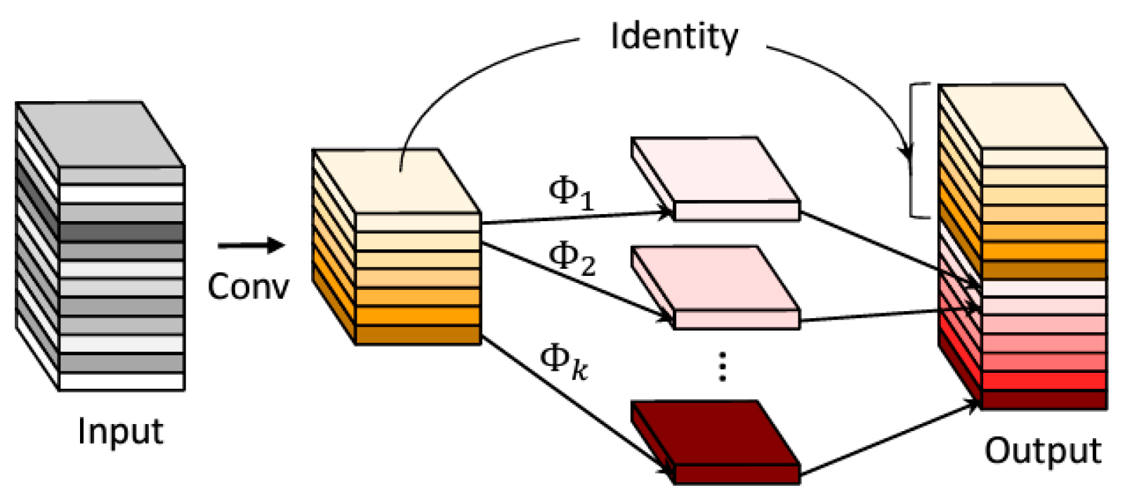
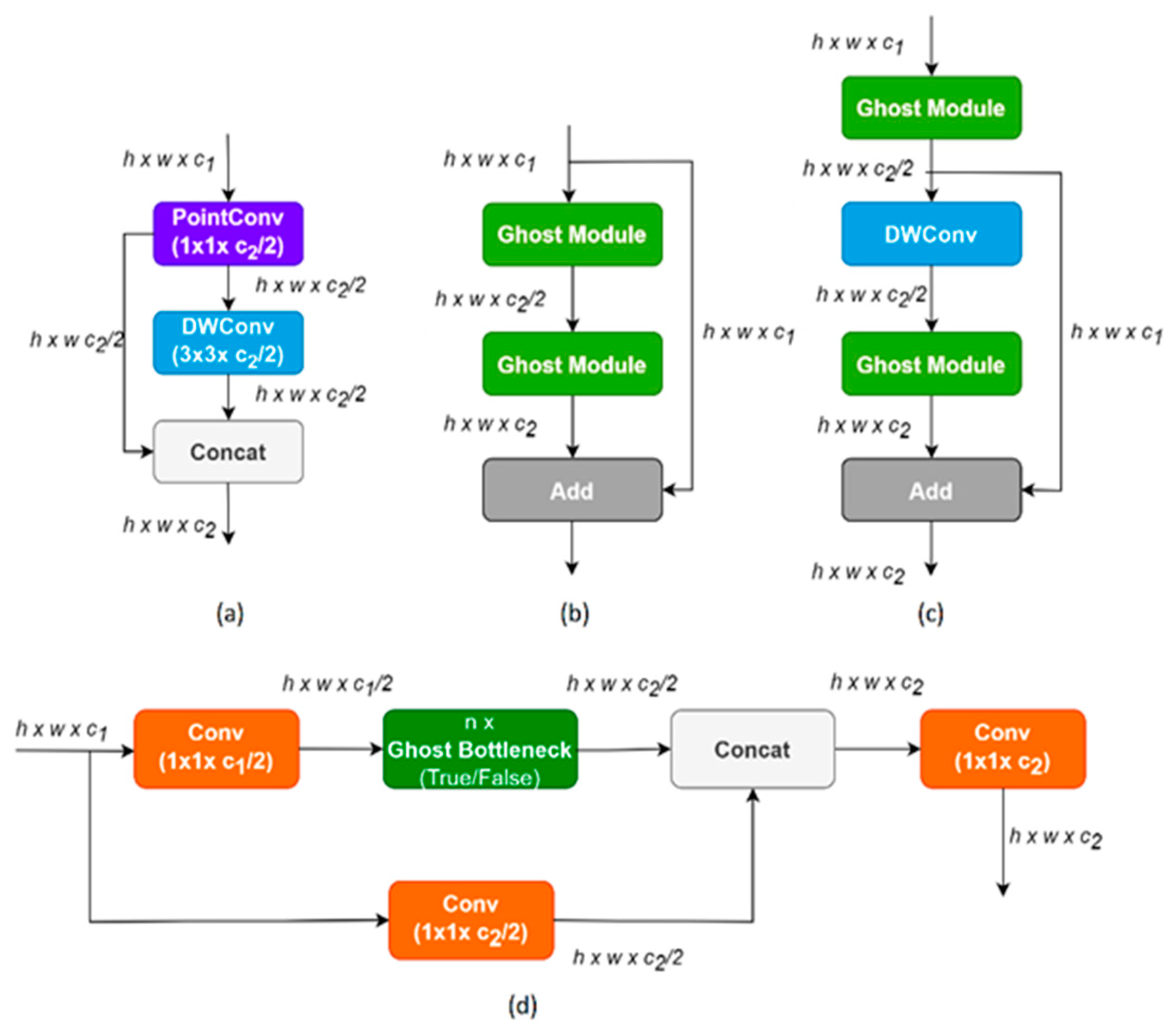
YOLOv5 is a three-part model comprising a backbone network, neck network, and head (Figure 1). It feeds the features extracted from input images through the backbone network into the neck network. The convolution module enhances the convergence of the model by performing batch normalisation, which enables the model to learn complex features using the SiLU activation function. The C3 module, including C3_1, performs the concatenation of different scale features and accelerates the network’s running time. The SPP module downsamples the input parallelly to retain context and edge details. The neck network integrates a parallel feature fusion network (FFN) and PAN to achieve effective feature fusion of low- and high-level information.
YOLOv5 uses the YOLOv3 head structure to perform object detection by regression computation and shows the prediction result. It generates the head of the object class, coordinates, and bounding boxes. By processing the input image, the convolutional layers extract feature maps at three levels (P3, P4, P5), which are then passed to the detection head for producing bounding boxes and class labels. The head network performs object detection by adopting a complete intersection over union (CIoU) loss, together with the NMS algorithm. As for the YOLOv5 v6.0 model, there are no major changes made to the backbone, but minor changes include replacing Focus with its equivalent convolution layer to enhance exportability and replacing SPP with SPPF for increased processing speed. More specifically, an optimised module called SPPF was adopted [28].
Whenever an image is entered into the model, a grid cell of a given size is placed over the image. The centre of an object falling in a given cell is responsible for estimating its coordinates and class. Each cell of the grid performs the task of estimating the dimensions of the bounding box, along with calculating their scores of confidence. Confidence scores signify the probability of an object being enclosed by the bounding box. The confidence score is mathematically represented in Equation (1):
c o n f i d e n c e   s c o r e = c o b j e c t × I o U t r u t h   p r e d
where c ( o b j e c t ) is the probability of the object present, varying between 0 and 1. The confidence score is assigned a value of zero when no object is detected. The Intersection over Union ( I o U t r u t h   p r e d ) quantifies how much the predicted bounding box overlaps with the ground truth box. A bounding box is characterised by x, y coordinates, width w, height h, and a confidence score, where the first four define its position and dimensions.

2.4. Ghost Module

This module aims to derive additional feature representations from the initial convolutional layer while reducing computation costs. For this purpose, another linear convolution process is performed by reducing the filters of convolution layers that have similarity in the intermediate feature maps computed by nonlinear convolution networks. In traditional convolution, for input data X   R c × h × w (where c represents the number of channels, h the height, and w the width), the generation of n feature maps is defined as shown in Equation (2):
Y = X f + b
where Y   R h × w × n represents the output feature map with n channels, height h, and width w, and f   R c × k × k × n denotes the convolutional filter with a kernel size of k × k. The symbol ∗ indicates the convolution operation, and b is the bias term. The number of FLOPs in this convolution process can be computed as n · c · h · w · k · k . This value is often substantial, since both the number of filters n and channels c are typically large.
The Ghost module considers that the output feature maps from traditional convolutional layers often exhibit significant redundancy, with many of them being highly similar. It assumes the existence of “ghosts”, which are generated by free-of-cost transformation. Therefore, m feature maps are generated using Y R m × h × w primary convolution, as in Equation (3):
Y = X f
where f     R c × k × k × m represents the filters used, with m     n , and the bias term is neglected. To obtain the desired n feature maps, a series of low-cost linear operations is applied to each feature in Y, generating s ghost features that are applied with Equation (4):
y i j = Φ i , j y i ,   i = 1 , . . . , m , j = 1 , . . . , s
where, y i   , denotes the i-th feature map in Y   , and Φ i , j represents the j-th linear operation of each y i   to generate the j-th ghost feature map y i j . The last Φ i , s is the identity mapping, as shown in Figure 2. Using Equation (4), n = m · s feature maps Y = [ y 11 , y 12 ,   . , y m s ] can be obtained from the output of a ghost module, as illustrated in Figure 2 [56]. The output feature map is then produced by combining the feature map generated through standard convolution with the one produced by ghost convolution.
Assuming a feature map of dimension c · h · w , a convolution kernel produces a feature map of dimension c · h · w after applying a regular convolution kernel of size k and a linear transform convolution kernel of size d. It can be concluded that the computation for the regular convolution to produce s ghost features after the transformation is c ·   h · w · c · k · k , and the computation of the ghost convolution is c s = h · w · c · k · k + ( s 1 ) · c s · h · w · d · d . A comparison of these two computations is presented in Equation (5):
r = c ·   h ·   w ·   c   ·   k   ·   k c s · h ·   w · c   · k   ·   k + s 1 · c s · h ·   w ·   d   ·   d = c   ·   k   ·   k 1 s · c   · k   ·   k + s 1 s ·   d   ·   d s · c s + c 1 s
where d × d and k × k have a similar size and sc. It can be observed that the computational cost of the standard convolution is s times greater than that of the Ghost convolution.
To minimise the computational complexity of convolutional neural networks and enhance their applicability on lightweight and resource-constrained devices, the Ghost module (Figure 3a) was adapted to the standard bottleneck structure to create the Ghost Bottleneck module [76]. There are two Ghost Bottleneck structures using Step = 1 and Step = 2 values. As shown in Figure 3b, in the first structure, the Ghost Bottleneck includes two Ghost modules, with a shortcut connection linking the inputs and outputs of these modules. Batch normalisation (BN) and ReLU nonlinearity are applied to the first layer, but ReLU is not applied to the other layer. In the second Ghost Bottleneck structure (Figure 3c), subsampling is applied by the layer, and in-depth cross-evolution is added between the two Ghost modules. To optimise efficiency, the primary convolution within the Ghost module uses pointwise convolution [56].
An optimised feature extraction structure based on the C3 module in YOLOv5, C3Ghost (Figure 3d), has been developed by adding Ghost Bottleneck to the C3 module (Ultralytics). The C3 module, with its multiple layers and redundant connections, provides a suitable environment for embedding Ghost modules into the structure, further reducing the computational cost and number of parameters while retaining feature extraction capabilities. The first standard convolution in the C3Ghost structure decreases the channel count to half of the output channels. Then, it comes to feature extraction through Ghost bottlenecks and residual branches set in serial. Thus, the depth semantic information of the input data is extracted through the two branches, and the two feature sets are combined using the concat module. After the concatenation process, convolution is applied for the enhancement of the combined features and context learning.

2.5. Attention Mechanism

Attention mechanisms contribute to a fair number of improvements for defect detection, especially on complex scenarios and small object detection, by dynamically estimating the relative importance of features in the input data. The role of the attention mechanism is to grant higher weights with regard to relevant features and allow the model to focus on important information and disregard the less relevant one, thereby enhancing model accuracy and efficiency. Some of them include Squeeze-and-Excitation Networks (SENets) [78], Coordinate Attention (CA) [79], the Normalisation-based Attention Module (NAM) [80], Efficient Channel Attention (ECA) [31], and the Convolutional Block Attention Module (CBAM) [81], which can be used as modules in network architectures to enhance the generalisation capabilities of the CNNs.
The ECA is an efficient channel attention method, inspired by the blocks of SENet for a good balance between performance and architectural simplicity (Figure 4).
The SENet attention mechanism uses spatial dimensions to pool and capture dependencies between channels through two fully connected layers. While this method achieved good results, it also increased computational complexity. The ECA module uses fast one-dimensional convolution in place of a fully connected layer, thereby reducing computational overhead and improved channel attention learning by capturing nonlinear information between channels. With this approach, the network has learned better capture of channel attention, reducing the number of parameters in the network and improving its performance [31].
The ECA module in Figure 4 takes the aggregated features from global average pooling (GAP), applies a fast 1D convolution in k dimension, and produces channel weights. Here k is adaptively calculated according to the channel dimension C. Representing the coverage rate of cross-channel information, k is the kernel size of the one-dimensional convolution and is proportional to the channel size C. There is mapping between the total channel size C and k, where the mapping ϕ is a linear function γ × k b , as in Equation (6):
ϕ ( C ) = γ × k b
Since the number of channels in convolutional networks is set to a power of 2, and the mapping relation with a linear function is simple, the linear function is obtained with a nonlinear function, as in Equation (7):
C = ϕ ( k ) = 2 ( γ × k b )
Thus, for a given channel size C, the kernel size k is obtained through an adaptive function defined in Equation (8):
k = ψ C = c   γ + b γ o d d
where k is the kernel size, c is the channel size, and γ and b are set to 2 and 1, respectively, to make the kernel size close to an odd number.

3. Proposed Method

YOLOv5, a single-stage real-time object detection model, is frequently encountered in different industrial scenarios and academic studies, with enhancements for defect detection tasks and mitigations in the network structure. The most important reasons for this are the model’s fast prediction capability, low latency, satisfactory accuracy performance, open-source structure, ability to run on limited-resource devices, and easy integration into different platforms. In this study, YOLOv5, which stands out in terms of accuracy and speed balance as a result of preliminary experiments, was taken as the basic architecture, and improvements were made for carbon footprint, real-time requirements, and use in resource-constrained devices. This YOLOv5s-based network enhancement with Ghost blocks, ECA mechanism, and P3–P4 head structure is proposed and named GLDD-YOLOv5 in this study. Figure 5 shows the proposed network structure.

3.1. Backbone

The base YOLOv5s model has approximately 7 M parameters, a computational cost of 15.9 GFLOPs, and a weight file size of 14.4 MB. The aim was to make the model lighter and more efficient by reducing these values in the context of speed and accuracy trade-offs. First, to reduce the computational complexity of the model, the CBS module in the backbone structure and neck structure of the YOLOv5s network was replaced with the Ghost convolution module. The backbone structure consists of deep convolutional layers to extract feature maps at hierarchically different scales from the input image. The GhostConv module replaces the standard convolution process with the Ghost convolution process, which provides more information with fewer parameters, resulting in deeper and more abstract representations without significant changes in accuracy. This results in lower computational cost, fewer parameters, and less memory consumption.
The C3 module (C3_1), which follows the CBS convolution blocks in the neck structure, is replaced by the ECAC3 attention module. The addition of this attention mechanism improves the learning of which features of the model are more important on a channel-by-channel basis. It reduces the computational burden by capturing nonlinear defect information across channels with a one-dimensional convolution. Weights are dynamically adjusted to emphasise important features more. This supports deeper and more abstract representation learning. With the ECAC3 change, the overall performance and flexibility of the model is improved, supporting the development of a more sensitive and efficient defect detection algorithm.

3.2. Neck

The neck part produces the feature pyramid by enriching the features extracted from the backbone at different resolutions. Upsample and concat operations are applied to ensure interaction between the feature maps. To lower the model’s computational complexity, the Ghost convolution module takes the role of the CBS module in the neck structure, much like in the backbone. C3_2 modules are also designed with C3Ghost modules. C3Gost is a C3 module based on Ghost convolution that provides a more efficient convolution process by minimising information loss in the convolution of both low-level detail and high-level semantic information in defects.

3.3. Head

In YOLOv5, feature maps are generated from the input image at three different levels. These feature maps are fed to the detection head of YOLOv5 for object detection and classification. While the P3 feature map has the highest resolution and the most input image detail, it covers smaller areas. The P4 feature map has a lower resolution and contains more depth channels than P3. The P5 feature map has the lowest spatial resolution, has less input image detail, covers larger areas, and contains the most depth channels. However, since the P5 feature map is large in size, the computational cost is high. When the dataset was analysed, it was observed that there are no very large defects in the defect size distribution. Therefore, the prediction head of the model was updated to detect small and medium-sized defects.
Because the P5 processes feature maps with a larger receptive field and more depth channels, it requires a significant amount of memory and FLOPs. In the ablation experiments (Section 4.5), removing P5 from the detection head reduced the computational load from 11.4 GFLOP to 8.4 GFLOP (−26.3%) and increased the inference speed from 138.8 FPS to 163.9 FPS (+18.1%). Meanwhile, the number of parameters dropped from 4.83 M to 3.96 M, which means that computational complexity was reduced for the model.
Despite this reduction in the head structure, small and medium-sized defect detection has been improved, where the sensitivity increased from 0.799 to 0.822 (+2.9%) and mAP@0.5 from 0.777 to 0.806 (+3.7%). These values confirm that removing P5 not only reduces the computational load but also improves performance due to the specific defect size distribution in the dataset.
Considering the dataset characteristics, resource limitations, and real-time efficiency requirements together, and as a result of ablation experiments, this architectural change is justified. A two-level head structure (P3 and P4) is proposed in the architecture.

4. Results

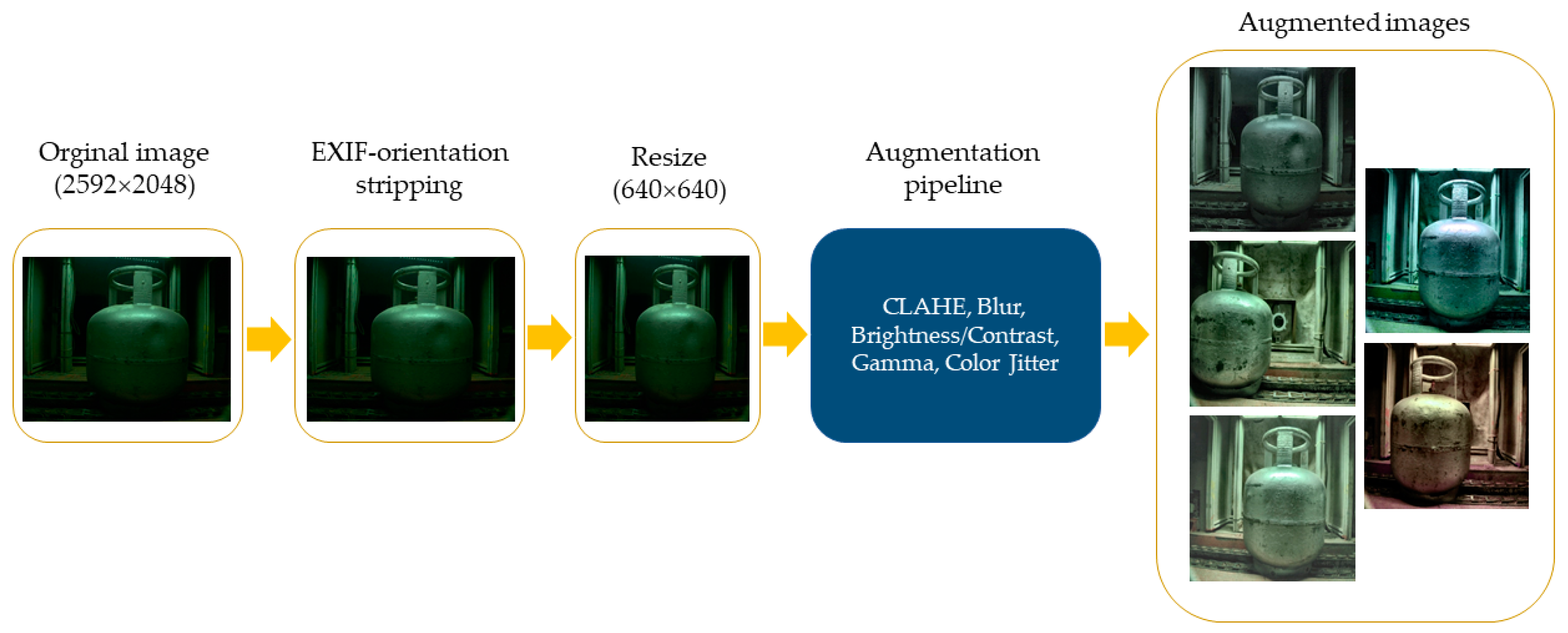
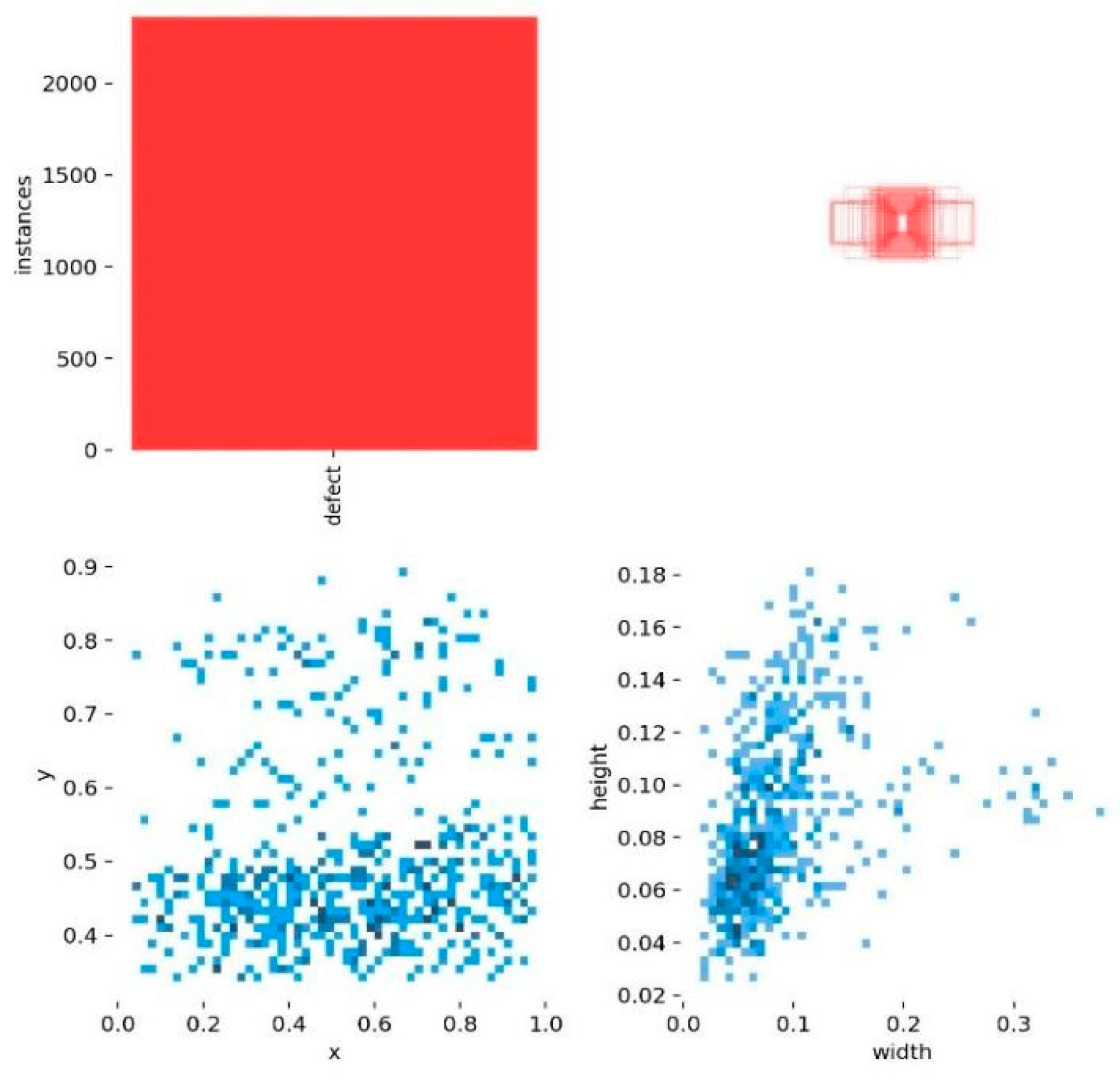
4.1. Experimental Dataset

The data used in the study were taken from an LPG company in Turkey, and the image data were acquired with a Basler acA2500-60uc USB 3.0 camera manufactured by Basler AG, located in Ahrensburg, Germany, which provides 60 FPS per second imaging at 5 MP resolution. The dataset contains a total of 2360 colour images with a size of 2592 × 2048. Since only LPG cylinders with surface defects were to be detected, the defects in each image were labelled using a single-class tool: https://www.makesense.ai/tool (accessed on 18 May 2024). The dataset was divided into training, validation, and test sets, at 70%, 15%, and 15% respectively. The test set was used to evaluate the defect detection accuracy of the trained model.
EXIF-orientation stripping and resizing to 640 × 640 were performed on the images. A data augmentation technique was applied to reduce the overfitting problem and increase the generalisation capability of the model. These included contrast-limited adaptive histogram equalisation (CLAHE), blur, random brightness and contrast adjustments, gamma corrections, and colour jitter. The augmentation pipeline was realised in code with the albumentations library, together with a bounding box format for YOLO. Figure 6 gives an overview of the dataset preparation and augmentation process.
Figure 7 shows the defect location and size distribution in the dataset images. The graphs at the bottom of Figure 7 show the location density of the defects. When the distribution of the x and y coordinates of the defects was examined, they were more dense in a certain region, and when the distribution of the bounding box dimensions (width-height) was examined, the defects were small and medium in size. The graph on the upper right of Figure 7 shows the areas where the defect bounding boxes overlap. This may indicate that the defects are repeated in similar locations.

4.2. Evaluation Metrics

Precision, recall, and mean average precision (mAP), which are standard metrics in object recognition, were used to evaluate model performance. Precision (P) is the proportion of the model’s true positive (TP) predictions out of all positive predictions. Recall (R) measures how successfully the model detects all true positive samples. Using the AP metric, which summarises the precision-recall curve and measures the precision at various recall levels for a given class, we found the average accuracy metrics (mAPs) of the model across all classes for different IoU thresholds. To evaluate the detection accuracy of the model, the overall average precision at the IoU (Intersection Over Union) threshold of 0.5, shown at mAP@0.5, was used.
In addition, FPS (frames per second), GFLOPs (giga floating point operations per second), model size, and number of parameters were considered to evaluate the real-time performance and computational efficiency of the model. Model size and number of parameters affect both memory footprint and inference time. GFLOPs are a measure of computational complexity, helping to compare the resource requirements for inference on different hardware platforms. FPS indicates how many image frames can be inferred in one second. Inference time refers to the time it takes the model to make a detection in one frame of image.
In this study, the inference time is taken as the sum of the pre-process, inference, and NMS times for each image as the average of the test image inferences. In addition, as an indicator of a lightweight and efficient green deep learning model, the carbon footprint generated during the running of the models was measured. The total carbon footprint during inference from test images was calculated by multiplying the energy consumption of the hardware (Watts), the execution time (hours), and the emission factor (kgCO2e/kWh) using the Python language CodeCarbon library (https://github.com/mlco2/codecarbon (accessed on 23 July 2024)).

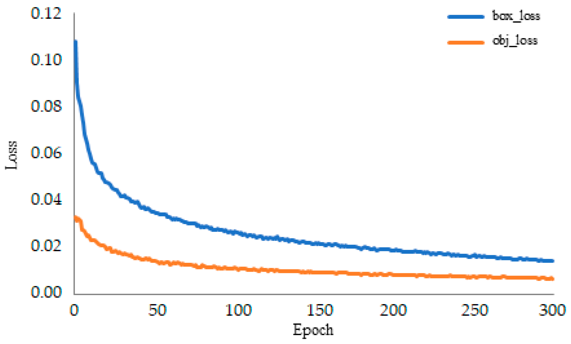
4.3. Implementation Details

The experiments were performed on a desktop workstation equipped with an Intel(R) Core(TM) i9-10920X @3.50 GHz processor and an NVIDIA GeForce RTX 2080 Ti GPU with 11,264 MB memory. The development environment includes Ubuntu 22.04.4 LTS, PyTorch 2.2.1, Python 3.12.2, and CUDA 12.1. The model was trained, then validated, and finally tested using the same hyperparameters and default values. The size of the original image fed into the model was 640 × 640. While training the weights, updating was performed using the SGD optimiser. The maximum number of epochs was 400, and the batch size was taken as 16. Momentum and weight reduction were taken as 0.937 and 0.0005, respectively. The initial learning rate was taken to be 0.01, and the method for reduction was changed to step by step in each epoch. While in the process of automatic frame detection, frames were optimised using a genetic algorithm.

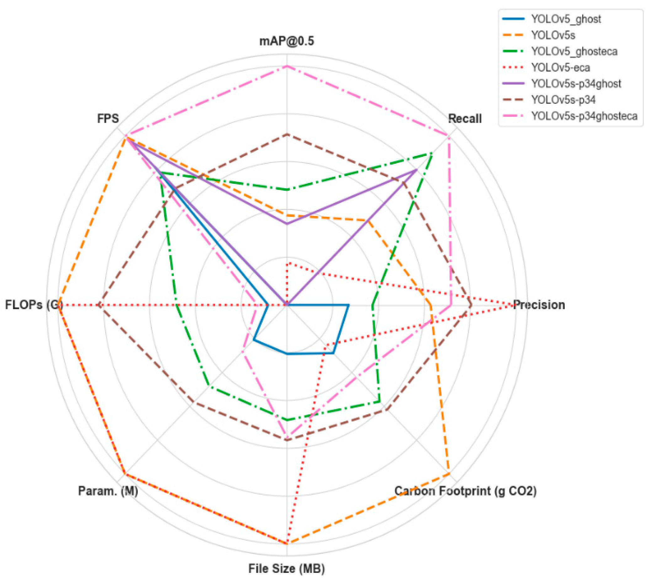
4.4. Comparison of YOLO Networks on a Custom Dataset

In the first phase of the study, the performances of different YOLO networks were evaluated with the dataset created specifically for this study in order to determine the base model. Considering the resource-constrained device requirements, the small-scale models of the models from YOLOv5 to YOLOv10 were trained with a personal dataset (no augmentation), and metrics were obtained. Since some YOLO versions do not have small models, those available as open source were evaluated. Table 1 shows the YOLO models compared and the values obtained.
As shown in Table 1, YOLOv5s seems to be a balanced model in terms of speed, accuracy, and efficiency, with 4.0 ms inference time, 0.79 mAP@0.5 accuracy, 15.9 GFLOPs computational cost, and 7.02 M parameters. The file size of 14.4 MB and low computational requirement make this model a suitable candidate to run on resource-constrained devices. The YOLOv6s model is relatively slow, with a 4.6 ms inference time, but yields 0.78 mAP@0.5 accuracy. However, due to 45.17 GFLOPs’ computational cost and 40.7 MB file size, it may be too large and computationally expensive to run on resource-constrained devices.
YOLOv8s is a satisfactory model in terms of inference time (5.4 ms). Although its accuracy (0.76 mAP@0.5) is reasonable, it is relatively better than YOLOv6s in terms of its 28.4 GFLOPs computational cost and 22.5 MB file size. YOLOv7, which is among the larger models, is slower and has lower performance, with a 8.3 ms inference time and a 0.59 mAP@0.5 accuracy value. With a 105.1 GFLOPs computational cost and a 74.8 MB file size, it is far from being preferred for use in edge devices compared to other models.
Although YOLOv9s offers one of the highest accuracy rates (0.78 mAP@0.5) and has higher computational requirements than YOLOv5s, with 38.7 GFLOPs and 9.74 M parameters. Likewise, its inference time (13.2 ms) is also relatively long. The inference speed (11.9 ms) and accuracy level (0.74 mAP@0.5) of the YOLO10s model are low compared to other models. Although it is a model that can be considered in scenarios requiring low resource usage, with its computational cost of 24.8 GFLOPs and 16.6 MB file size, it lags behind YOLOv5s and YOLOv9s in terms of accuracy. In light of all these, the YOLOv5s model stands out as the most suitable basic model for a system that will run on resource-constrained devices in terms of speed, accuracy, and computational cost.

4.5. Ablation Experiments

In the first phase of the study, modifications were made to the architecture of the basic model YOLOv5s with a Ghost module, ECA mechanism, and P3–P4 head, and ablation experiments were performed to verify the effectiveness of the proposed new model. The basic model was modified in the spine, neck, and head structure to achieve the optimal balance in terms of accuracy, energy consumption, weight, and real-time operation for resource-constrained devices. The impact of each modification on model accuracy, speed, computational efficiency, file size, and carbon footprint were analysed. The ablation experiment results of each module effect obtained by taking the input image size 640 × 640 are shown in Table 2.
The Ghost module, widely used in model lightweighting, was implemented in the YOLOv5s model architecture by replacing the standard convolution blocks with Ghost convolution and C3Ghost blocks. This change reduced the computational load, number of parameters, and file size of the model by close to 50%. This provides a very favourable memory footprint for edge devices. However, although it provides satisfactory performance in terms of accuracy and speed, it lags behind YOLOV5s. A total carbon footprint of 0.136 gCO2e was generated during the extraction.
The ECA attention mechanism is known to improve the feature extraction capability of the channels in the network. Studies comparing the ECA attention mechanism with other attention mechanisms such as CA and CBAM in the YOLOv5s network have confirmed that the addition of ECA to the backbone network is the most effective compared with other attention mechanisms [30,82]. The YOLOv5-ECA model with only ECA modification surpasses the baseline model with a precision of 0.841, but is slightly lower than the baseline model, with an accuracy of 0.76 mAP@0.5. In terms of FPS, number of parameters, file size, and carbon footprint values, it remains the same as the baseline model.
The combined Ghost and ECA modifications resulted in an accuracy value of 0.777 mAP@0.5, which is an insignificant accuracy improvement over the baseline model. In this modification, the three-head structure in the original YOLOv5s has not been changed. The model outperformed the baseline model by 138.8 FPS. The most obvious advantages of this modification are an increase in computational efficiency with 11.4 GFLOPs, a reduction in the number of parameters with 4.83 M parameters, and a reduction in file size with 10.1 MB. A carbon footprint of 0.150 gCO2e was measured during inference.
The P34 modification of the YOLOv5s model (YOLOv5-p34), which was created by removing the P5 head structure and leaving the P3 and P4 heads, offers a strong balance in terms of accuracy and speed. YOLOv5s-P34 shows high performance compared to YOLOv5s in terms of accuracy, with 0.79 mAP@0.5 and a speed with 175 FPS. At the same time, the number of parameters, file size, and computational load are low. The carbon footprint value was 0.143 gCO2e. In order to further lighten this structure, P34 and Ghost modifications were combined to create the YOLOv5-P34-Ghost model. Although the model showed a lower value than P34 and Ghost-ECA modifications, with an accuracy value of 0.769 mAP@0.5, and a decrease compared to YOLOv5-P34, with an extraction value of 158.7 FPS, it had the lowest value among all modifications, with a computational load of 7.3 GFLOPs, 2.80 M parameters, and 6.1 MB file size.
The ECA mechanism was added to this structure in order to increase the accuracy by improving the feature extraction capability without losing the gains obtained with the YOLOv5-P34-Ghost model. The YOLOv5-P34-Ghost-ECA modification achieved the highest accuracy rates of 0.822 precision, 0.785 recall, and 0.806 mAP@0.5. The model provides fast and efficient inference performance with an inference rate of 163.9 FPS and a computational load of 8.4 GFLOPs. With 3.96 M parameters and a 10.7 MB file size, it produced a carbon footprint of 0.145 gCO2e during inference. This proposed YOLOv5-P34-Ghost-ECA modification is named GLDD-YOLOv5 for the study.
The box loss and object loss curve of the proposed model over 300 epochs during the training process are shown in Figure 8. Box loss refers to the deviation between the predicted bounding box and the actual value. Object loss is a type of confidence loss that determines whether an object is present in the grid and calculates the confidence level of the model. At around Epoch 250, both loss values stabilised and decreased to very low levels. The graph shows that the model has undergone an effective learning process, improving its ability to accurately predict object location and presence.
This ablation study analysed the effects of each optimised modification on the accuracy, speed, and energy efficiency of LPG cylinder surface defect detection. As a result of the ablation experiments, it was found that the Ghost and ECA modifications provide positive effects on both accuracy and energy efficiency, while the P34 structure improves overall performance. All results obtained from the ablation experiments are shown in Figure 9.

4.6. Comparison with Large-Scale Object Detection Network

Transformer structures, which are widely used in natural language processing, have recently been used in computer vision and have become an alternative to CNN-based models. In order to make an alternative evaluation, RT-DETR [83], an optimised transformer model for real-time object detection, was trained on the dataset, and the performance of the model was tested on the dataset. The results obtained are given comparatively in Table 3.
Table 3 shows that the proposed GLDD-YOLOv5 model runs with higher mAP@0.5 accuracy, higher FPS, and lower FLOP values than the RT-DETR model. Although it is not correct to evaluate RT-DETR and GLDD-YOLOv5 models in the same category, this was intended to emphasise the superiority of the proposed model over the large-scale object detection network in terms of defect detection accuracy.

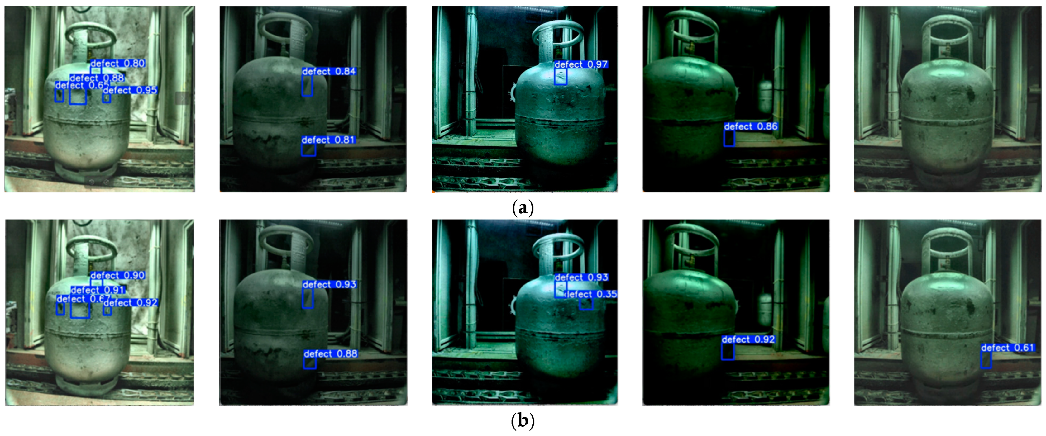
4.7. Qualitative Visualisation of the Detection Results

This section presents a qualitative performance comparison between the proposed GLDD-YOLOv5 model and the baseline YOLOv5s model for defect detection. In the process environment, there are challenges such as the fact that the background (non-object parts) contains defect-like structures, there are hard-to-see defects on the lower parts of LPG cylinder surfaces, and the colours of the objects in the background and the object to be detected are very close to each other. In addition, there are likely to be changes in the ambient light level from time to time. The models were run for the defect detection task on test images simulating ambient conditions with different image processing techniques, and some of the results are shown in Figure 10. Figure 10a illustrates the defect detection results of the basic YOLOv5s model, while Figure 10b illustrates the defect detection results of the GLDD-YOLOv5 model.
The proposed GLDD-YOLOv5 model showed relatively high confidence scores in the detection of small or less noticeable defects in low light, bright images, contrast, and complex background conditions. YOLOv5s failed to detect some defects (Figure 10, third and fifth columns) or gave a lower confidence score (Figure 10, second and fourth columns). Furthermore, the GLDD-YOLOv5 model has relatively high localisation accuracy in the bounding box placement around the detected defects (Figure 10, first, second, and fourth columns).
This comparison reveals that the GLDD-YOLOv5 model outperforms the baseline YOLOv5s in defect detection under challenging conditions such as very small defect areas, different lighting conditions, similar backgrounds, and complex surfaces. This demonstrates the potential of GLDD-YOLOv5 to be applied when the accuracy and reliability of defect detection is essential.

5. Discussion

Overall, the proposed model performed well in terms of accuracy, speed, computational load, and memory footprint balance. It was observed that GLDD-YOLOv5 has higher adaptability and more capability in defect detection in a complex environment and under different lighting conditions compared to existing state-of-the-art models. It also showed relatively higher accuracy in bounding box localisation.
The GLDD-YOLOv5 model proposed in this study provides a 4.6% improvement in accuracy (mAP50) compared to YOLOv5s, while improving the computational cost by 44% with 8.4 GFLOPs, the number of parameters by 45% with 3.96 M, and the file size by 26% with 10.7 MB. Although it shows a 6% decrease in inference speed (from 175 FPS to 163.9 FPS), this is minimal compared to other models. It produced a total carbon footprint of 0.145 gCO2e in the inference phase with the test dataset.
Evaluation of the carbon footprint in the study revealed that optimisation of the models is critical not only in terms of computational efficiency but also in terms of sustainability. The proposed model provides a perspective on developing environmentally friendly, effective, efficient, and fast object detection solutions in resource-limited environments such as edge devices.
In light of these evaluations, GLDD-YOLOv5 performed better than other models in the field of industrial defect detection and managed to increase the accuracy rate without sacrificing too much speed. GLDD-YOLOv5 appears to be a particularly high-performance and efficient solution.
Nevertheless, there were some limitations to the study. Due to the ongoing operation of the industrial plant, the available was limited in scope and focused on specific defect types. Deployment of the defect detection system will facilitate expansion of the learning capacity of the model by diversifying the dataset to cover a wider range of data. Furthermore, evaluation of the model’s performance on different datasets was limited, as there is no open dataset serving a similar purpose in the existing literature. Future studies will investigate the generalisation capability of the model by evaluating it with various datasets. In addition, some complex backgrounds, which are not always possible under physical conditions, as well as limitations in adjusting camera viewing angles, which are necessary for optimal conditions, may lead to off-target false detections. The performance of the models can be further optimised in future studies by applying more lightweight techniques such as quantisation [84], model pruning [60,85] and information distillation [86].

6. Conclusions

This paper presents a high-precision defect detection model based on YOLOv5, specifically tailored for resource-constrained devices. A robust and efficient model, GLDD-YOLOv5, is proposed by integrating an ECA mechanism to increase the feature extraction capacity of the backbone network, Ghost modules to lighten the model architecture, and a P34 head structure to increase the detection speed. By replacing the backbone of the YOLOv5 network with both Ghost modules and ECA mechanisms, feature extraction capabilities were improved without compromising detection accuracy, and small to medium-sized defects in images were targeted. Adjustments to the model’s head structure further concentrated detection on small and medium-sized areas, effectively balancing detection accuracy and extraction speed. The contribution of each module has been demonstrated through ablation studies, showing the impact of each modification on model performance. The proposed model outperforms the other six YOLO family versions, achieving a remarkable balance of performance with an average detection accuracy of 80.6% (mAP@0.5), computational efficiency of 8.4 GFLOPs, 3.96 M parameters, and memory footprint of 10.7 MB. In terms of real-time performance, the model achieved 163.9 FPS on RTX2080Ti and produced a total carbon footprint of 0.549 × 10⁻³ gCO2e, demonstrating its environmental friendliness as well as its speed of inference compared to other models.
Considering these strengths, GLDD-YOLOv5 stands out as an important solution for LPG cylinder surface defect detection. Its high detection accuracy, low computational cost, adaptability to constrained environments, and environmental friendliness make it a suitable candidate for use in real-world and defect detection applications.
This study is limited to finding defects on the surface of LPG cylinder surfaces, and hence their location. The location of the defect on the surface, the type of defect, and the shape of the defect were not studied. In future studies, with expansion of the dataset, a different classification will be created by determining the type and location of the defect. In addition, it is planned to evaluate the performance of the proposed model by applying it to inexpensive edge devices such as Raspberry Pi 5 and Nvidia Jetson Nano. Future research could focus on further development of this architecture, potentially increasing its applicability to a wider range of surface defect detection scenarios in various industrial applications.

Funding

This research was funded by AYGAZ A.Ş., no grant number was assigned.

Institutional Review Board Statement

Not applicable.

Informed Consent Statement

Not applicable.

Data Availability Statement

Restrictions apply to the availability of these data. Data were obtained from funders and are available from the authors with the permission of the funders.

Acknowledgments

The author deeply appreciates the team at AYGAZ A.Ş. for their essential contribution in gathering the images that were used to create the dataset for this study.

Conflicts of Interest

The author declares no conflicts of interest. The funder had no role in the design of the study, analyses, interpretation of data, writing of the manuscript or decision to publish the results.

References

  1. Venegas-Vásconez, D.; Ayabaca-Sarria, C.; Reina-Guzmán, S.; Tipanluisa-Sarchi, L.; Farías-Fuentes, Ó. Liquefied Petroleum Gas Systems: A Review on Design and Sizing Guidelines. Ingenius Rev. Cienc. Tecnol. 2024, 31, 81–93. [Google Scholar]
  2. Turkish Standards Institute (TSE). TS EN 1439: LPG Equipment and Accessories—Periodic Inspection and Testing of LPG Cylinders. Available online: https://intweb.tse.org.tr/Standard/Standard/StandardAra.aspx (accessed on 27 December 2024).
  3. Singh, S.A.; Desai, K.A. Automated surface defect detection framework using machine vision and convolutional neural networks. J. Intell. Manuf. 2023, 34, 1995–2011. [Google Scholar] [CrossRef]
  4. Bai, J.; Wu, D.; Shelley, T.; Schubel, P.; Twine, D.; Russell, J.; Zeng, X.; Zhang, J. A comprehensive survey on machine learning-driven material defect detection: Challenges, solutions, and future prospects. arXiv 2024, arXiv:2406.07880. [Google Scholar] [CrossRef]
  5. Jung, H.; Lee, C.; Park, G. Fast and non-invasive surface crack detection of press panels using image processing. Proced. Eng. 2017, 188, 72–79. [Google Scholar] [CrossRef]
  6. Shi, T.; Kong, J.-Y.; Wang, X.-D.; Liu, Z.; Zheng, G. Improved Sobel algorithm for defect detection of rail surfaces with enhanced efficiency and accuracy. J. Cent. S. Univ. 2016, 23, 2867–2875. [Google Scholar] [CrossRef]
  7. Liu, W.; Yan, Y. Automated surface defect detection for cold-rolled steel strip based on wavelet anisotropic diffusion method. Int. J. Ind. Syst. Eng. 2014, 17, 224. [Google Scholar] [CrossRef]
  8. Neogi, N.; Mohanta, D.K.; Dutta, P.K. Defect detection of steel surfaces with global adaptive percentile thresholding of gradient image. J. Inst. Eng. India Ser. B 2017, 98, 557–565. [Google Scholar] [CrossRef]
  9. Hassanin, A.-A.I.M.; El-Samie, F.E.A.; El Banby, G.M. A real-time approach for automatic defect detection from PCBs based on SURF features and morphological operations. Multimed. Tools Appl. 2019, 78, 34437–34457. [Google Scholar] [CrossRef]
  10. Saberironaghi, A.; Ren, J.; El-Gindy, M. Defect detection methods for industrial products using deep learning techniques: A review. Algorithms 2023, 16, 95. [Google Scholar] [CrossRef]
  11. Li, J.; Pan, H.; Li, J. ESD-YOLOv5: A Full-Surface Defect Detection Network for Bearing Collars. Electronics 2023, 12, 16. [Google Scholar] [CrossRef]
  12. Su, P.; Han, H.; Liu, M.; Yang, T.; Liu, S. MOD-YOLO: Rethinking the YOLO Architecture at the Level of Feature Information and Applying It to Crack Detection. Expert Syst. Appl. 2024, 237, 121346. [Google Scholar] [CrossRef]
  13. Chen, X.; Wu, Y.; He, X.; Ming, W. A comprehensive review of deep learning-based PCB defect detection. IEEE Access 2023, 11, 139017–139038. [Google Scholar] [CrossRef]
  14. Liu, J.; Hu, M.; Dong, J.; Lu, X. Summary of insulator defect detection based on deep learning. Electr. Power Syst. Res. 2023, 224, 109688. [Google Scholar] [CrossRef]
  15. Demir, K.; Ay, M.; Cavas, M.; Demir, F. Automated steel surface defect detection and classification using a new deep learning-based approach. Neural Comput. Appl. 2023, 35, 8389–8406. [Google Scholar] [CrossRef]
  16. Li, Z.; Wei, X.; Hassaballah, M.; Li, Y.; Jiang, X. A deep learning model for steel surface defect detection. Complex Intell. Syst. 2024, 10, 885–897. [Google Scholar] [CrossRef]
  17. Singh, S.A.; Kumar, A.S.; Desai, K.A. Comparative assessment of common pre-trained CNNs for vision-based surface defect detection of machined components. Expert Syst. Appl. 2023, 218, 119623. [Google Scholar] [CrossRef]
  18. Li, C.; Li, J.; Li, Y.; He, L.; Fu, X.; Chen, J. Fabric defect detection in textile manufacturing: A survey of the state of the art. Secur. Commun. Netw. 2021, 2021, 9948808. [Google Scholar] [CrossRef]
  19. Yi, L.P.; Akbar, M.F.; Wahab, M.N.A.; Rosdi, B.A.; Fauthan, M.A.; Shrifan, N.H.M.M. The prospect of artificial intelligence-based wood surface inspection: A review. IEEE Access 2024, 12, 84706–84725. [Google Scholar] [CrossRef]
  20. Girshick, R.; Donahue, J.; Darrell, T.; Malik, J. Rich feature hierarchies for accurate object detection and semantic segmentation. In Proceedings of the 2014 IEEE Conference on Computer Vision and Pattern Recognition, Columbus, OH, USA, 23–28 June 2014; pp. 580–587. [Google Scholar] [CrossRef]
  21. Girshick, R. Fast R-CNN. In Proceedings of the IEEE International Conference on Computer Vision 2015, Santiago, Chile, 7–13 December 2015; pp. 1440–1448. [Google Scholar]
  22. Ren, S.; He, K.; Girshick, R.; Sun, J. Faster R-CNN: Towards real-time object detection with region proposal networks. IEEE Trans. Pattern Anal. Mach. Intell. 2017, 39, 1137–1149. [Google Scholar] [CrossRef]
  23. Liu, W.; Anguelov, D.; Erhan, D.; Szegedy, C.; Reed, S.; Fu, C.Y.; Berg, A.C. SSD: Single Shot MultiBox Detector. In Computer Vision—ECCV 2016; Lecture Notes in Computer Science; Leibe, B., Matas, J., Sebe, N., Welling, M., Eds.; Springer: Cham, Switzerland, 2016; Volume 9905. [Google Scholar] [CrossRef]
  24. Redmon, J.; Divvala, S.; Girshick, R.; Farhadi, A. You only look once: Unified, real-time object detection. In Proceedings of the 2016 IEEE Conference on Computer Vision and Pattern Recognition (CVPR), Las Vegas, NV, USA, 27–30 June 2016. [Google Scholar]
  25. Xu, J.; Zhou, W.; Fu, Z.; Zhou, H.; Li, L. A survey on green deep learning. arXiv 2021, arXiv:2111.05193. [Google Scholar]
  26. Schwartz, R.; Dodge, J.; Smith, N.A.; Etzioni, O. Green AI. Commun. ACM 2020, 63, 54–63. [Google Scholar] [CrossRef]
  27. Bochkovskiy, A.; Wang, C.-Y.; Liao, H.-Y.M. YOLOv4: Optimal speed and accuracy of object detection. arXiv 2020, arXiv:2004.10934. [Google Scholar]
  28. Jocher, G.; Chaurasia, A.; Qiu, J.; Stoken, N. YOLOv5 v6.0. GitHub Repository. 2021. Available online: https://github.com/ultralytics/yolov5/releases/tag/v6.0 (accessed on 2 October 2024).
  29. Ren, F.; Fei, J.; Li, H.; Doma, B.T. Steel surface defect detection using improved deep learning algorithm: ECA-SimSPPF-SIoU-YOLOv5. IEEE Access 2024, 12, 32545–32553. [Google Scholar] [CrossRef]
  30. Zhang, D.-Y.; Zhang, W.; Cheng, T.; Zhou, X.-G.; Yan, Z.; Wu, Y.; Zhang, G.; Yang, X. Detection of wheat scab fungus spores utilizing the YOLOv5-ECA-ASFF network structure. Comput. Electron. Agric. 2023, 210, 107953. [Google Scholar] [CrossRef]
  31. Wang, Q.; Wu, B.; Zhu, P.; Li, P.; Zuo, W.; Hu, Q. ECA-net: Efficient channel attention for deep convolutional neural networks. In Proceedings of the 2020 IEEE/CVF Conference on Computer Vision and Pattern Recognition (CVPR), Seattle, WA, USA, 13–19 June 2020. [Google Scholar]
  32. Lu, L.; Chen, Z.; Wang, R.; Liu, L.; Chi, H. YOLO-Inspection: Defect detection method for power transmission lines based on enhanced YOLOv5s. J. Real Time Image Process. 2023, 20, 104. [Google Scholar] [CrossRef]
  33. Huang, J.; Chen, J.; Wang, H. A lightweight and efficient one-stage detection framework. Comput. Electr. Eng. 2023, 105, 108520. [Google Scholar] [CrossRef]
  34. Liu, M.; Chen, Y.; Xie, J.; He, L.; Zhang, Y. LF-YOLO: A lighter and faster YOLO for weld defect detection of X-ray image. IEEE Sens. J. 2023, 23, 7430–7439. [Google Scholar] [CrossRef]
  35. Hou, W.; Wen, S.; Li, P.; Feng, S. Surface defect detection of fabric based on improved Faster R-CNN. In Proceedings of the 2023 IEEE International Conference on Sensors, Electronics and Computer Engineering (ICSECE), Jinzhou, China, 18–20 August 2023; pp. 600–604. [Google Scholar]
  36. Wang, J.; Xu, G.; Yan, F.; Wang, J.; Wang, Z. Defect transformer: An efficient hybrid transformer architecture for surface defect detection. Measurement 2023, 211, 112614. [Google Scholar] [CrossRef]
  37. Liu, X.; Gao, J. Surface defect detection method of hot rolling strip based on improved SSD model. In Database Systems for Advanced Applications, Proceedings of the DASFAA 2021 International Workshops: GDMA, MLDLDSA, MobiSocial, and MUST, Taipei, Taiwan, 11–14 April 2021; Springer International Publishing: Berlin/Heidelberg, Germany; pp. 209–222. [Google Scholar]
  38. Dosovitskiy, A.; Beyer, L.; Kolesnikov, A.; Weissenborn, D.; Zhai, X.; Unterthiner, T.; Dehghani, M.; Minderer, M.; Heigold, G.; Gelly, S.; et al. An image is worth 16x16 words: Transformers for image recognition at scale. arXiv 2020, arXiv:2010.11929. [Google Scholar]
  39. Liu, Z.; Gao, J. Swin Transformer: Hierarchical vision transformer using shifted windows. arXiv 2021, arXiv:2103.14030. [Google Scholar]
  40. Zhu, W.; Zhang, H.; Zhang, C.; Zhu, X.; Guan, Z.; Jia, J. Surface defect detection and classification of steel using an efficient Swin Transformer. Adv. Eng. Inform. 2023, 57, 102061. [Google Scholar] [CrossRef]
  41. Zhou, H.; Yang, R.; Hu, R.; Shu, C.; Tang, X.; Li, X. ETDNet: Efficient transformer-based detection network for surface defect detection. IEEE Trans. Instrum. Meas. 2023, 72, 2525014. [Google Scholar] [CrossRef]
  42. Shang, H.; Sun, C.; Liu, J.; Chen, X.; Yan, R. Defect-aware transformer network for intelligent visual surface defect detection. Adv. Eng. Inform. 2023, 55, 101882. [Google Scholar] [CrossRef]
  43. Khan, A.; Rauf, Z.; Sohail, A.; Rehman, A.; Asif, H.; Asif, A.; Farooq, U. A survey of the Vision Transformers and their CNN-Transformer based variants. arXiv 2023, arXiv:2305.09880. [Google Scholar] [CrossRef]
  44. Lee, S.I.; Koo, K.; Lee, J.H.; Lee, G.; Jeong, S.; Kim, H.O.S. Vis. Transform. Models Mob. /Edge Devices: A Survey. Multimed. Syst. 2024, 30, 109. [Google Scholar] [CrossRef]
  45. Maurício, J.; Domingues, I.; Bernardino, J. Comparing vision transformers and convolutional neural networks for image classification: A literature review. Appl. Sci. 2023, 13, 9. [Google Scholar] [CrossRef]
  46. Tao, Y.; Zongyang, Z.; Jun, Z.; Xinghua, C.; Fuqiang, Z. Low-altitude small-sized object detection using lightweight feature-enhanced convolutional neural network. J. Syst. Eng. Electron. 2021, 32, 841–853. [Google Scholar] [CrossRef]
  47. Kamath, V.; Renuka, A. Deep learning based object detection for resource-constrained devices: Systematic review, future trends and challenges ahead. Neurocomputing 2023, 531, 34–60. [Google Scholar] [CrossRef]
  48. Xiang, C.; Guo, J.; Cao, R.; Deng, L. A crack-segmentation algorithm fusing transformers and convolutional neural networks for complex detection scenarios. Autom. Constr. 2023, 152, 104894. [Google Scholar] [CrossRef]
  49. Taye, M.M. Theoretical understanding of convolutional neural network: Concepts, architectures, applications, future directions. Computation 2023, 11, 52. [Google Scholar] [CrossRef]
  50. He, K.; Zhang, X.; Ren, S.; Sun, J. Deep residual learning for image recognition. In Proceedings of the 2016 IEEE Conference on Computer Vision and Pattern Recognition (CVPR), Las Vegas, NV, USA, 27–30 June 2016; pp. 770–778. [Google Scholar]
  51. Simonyan, K.; Zisserman, A. Very deep convolutional networks for large-scale image recognition. arXiv 2014, arXiv:1409.1556. [Google Scholar]
  52. Huang, G.; Liu, Z.; van der Maaten, L.; Weinberger, K.Q. Densely connected convolutional networks. In Proceedings of the IEEE Conference on Computer Vision and Pattern Recognition 2017, Honolulu, HI, USA, 21–26 July 2017; pp. 4700–4708. [Google Scholar]
  53. Iandola, F.N.; Han, S.; Moskewicz, M.W.; Ashraf, K.; Dally, W.J.; Keutzer, K. SqueezeNet: AlexNet-level accuracy with 50× fewer parameters and <0.5 MB model size. arXiv 2016, arXiv:1602.07360. [Google Scholar]
  54. Howard, G.; Sandler, M.; Zhu, M.; Zhmoginov, A.; Chen, L.-C. MobileNets: Efficient Convolutional Neural Networks for Mobile Vision Applications. arXiv 2017, arXiv:1704.04861. [Google Scholar] [CrossRef]
  55. Zhang, X.; Zhou, X.; Lin, M.; Sun, J. ShuffleNet: An extremely efficient convolutional neural network for mobile devices. In Proceedings of the 2018 IEEE/CVF Conference on Computer Vision and Pattern Recognition, Salt Lake City, UT, USA, 18–23 June 2018; pp. 6848–6856. [Google Scholar]
  56. Han, K.; Wang, Y.; Tian, Q.; Guo, J.; Xu, C.; Xu, C. GhostNet: More features from cheap operations. In Proceedings of the 2020 IEEE/CVF Conference on Computer Vision and Pattern Recognition (CVPR), Seattle, WA, USA, 13–19 June 2020; pp. 1580–1589. [Google Scholar]
  57. Gholami, A.; Kwon, K.; Wu, B.; Tai, Z.; Yue, X.; Jin, P.; Keutzer, K. SqueezeNext: Hardware-aware neural network design. In Proceedings of the IEEE Conference on Computer Vision and Pattern Recognition Workshops 2018, Salt Lake City, UT, USA, 18–22 June 2018; pp. 1638–1647. [Google Scholar]
  58. Sandler, M.; Howard, A.; Zhu, M.; Zhmoginov, A.; Chen, L.-C. MobileNetV2: Inverted residuals and linear bottlenecks. In Proceedings of the 2018 IEEE/CVF Conference on Computer Vision and Pattern Recognition, Salt Lake City, UT, USA, 18–23 June 2018; pp. 4510–4520. [Google Scholar]
  59. Ma, N.; Zhang, X.; Zheng, H.-T.; Sun, J. ShuffleNet V2: Practical guidelines for efficient CNN architecture design. arXiv 2018, arXiv:1807.11164. [Google Scholar]
  60. Zhang, G.; Liu, S.; Nie, S.; Yun, L. YOLO-RDP: Lightweight Steel Defect Detection through Improved YOLOv7-Tiny and Model Pruning. Symmetry 2024, 16, 458. [Google Scholar] [CrossRef]
  61. Zhou, S.; Ao, S.; Yang, Z.; Liu, H. Surface defect detection of steel plate based on SKS-YOLO. IEEE Access 2024, 12, 91499–91510. [Google Scholar] [CrossRef]
  62. Huang, H. TLI-YOLOv5: A lightweight object detection framework for transmission line inspection by unmanned aerial vehicle. Electronics 2023, 12, 3340. [Google Scholar] [CrossRef]
  63. Sapkota, R.; Meng, Z.; Churuvija, M.; Du, X.; Ma, Z.; Karkee, M. Comprehensive performance evaluation of YOLOv10, YOLOv9 and YOLOv8 on detecting and counting fruitlet in complex orchard environments. arXiv 2024, arXiv:2407.12040. [Google Scholar] [CrossRef]
  64. Lin, T.Y.; Dollár, P.; Girshick, R.; He, K.; Hariharan, B.; Belongie, S. Feature pyramid networks for object detection. In Proceedings of the IEEE Conference on Computer Vision and Pattern Recognition 2017, Honolulu, HI, USA, 21–26 July 2017; pp. 2117–2125. [Google Scholar]
  65. Wang, C.-Y.; Liao, H.-Y.M.; Wu, Y.-H.; Chen, P.-Y.; Hsieh, J.-W.; Yeh, I.-H. CSPNet: A new backbone that can enhance learning capability of CNN. In Proceedings of the 2020 IEEE/CVF Conference on Computer Vision and Pattern Recognition Workshops (CVPRW), Seattle, WA, USA, 14–19 June 2020; pp. 1571–1580. [Google Scholar]
  66. Ma, Z.; Li, M.; Wang, Y. PAN: Path integral based convolution for deep graph neural networks. arXiv 2019, arXiv:1904.10996. [Google Scholar] [CrossRef]
  67. Hussain, M.; Khanam, R. In-depth review of YOLOv1 to YOLOv10 variants for enhanced photovoltaic defect detection. Solar 2024, 4, 351–386. [Google Scholar] [CrossRef]
  68. Sohan, M.; Ram, T.S.; Reddy, C.V.R. A review on YOLOv8 and its advancements. In Proceedings of the International Conference on Data Intelligence and Cognitive Informatics 2024, Tirunelveli, India, 18–20 November 2024; Springer: Singapore, 2024; pp. 529–545. [Google Scholar]
  69. Alif, M.A.R.; Hussain, M. YOLOv1 to YOLOv10: A comprehensive review of YOLO variants and their application in the agricultural domain. arXiv 2024, arXiv:2406.10139. [Google Scholar] [CrossRef]
  70. Xu, X.; Jiang, Y.; Chen, W.; Huang, Y.; Zhang, Y.; Sun, X. Damo-YOLO: A report on real-time object detection design. arXiv 2022, arXiv:2406.10139. [Google Scholar] [CrossRef]
  71. Ultralytics. Home. 2023. Available online: https://docs.ultralytics.com/ (accessed on 5 November 2024).
  72. Solawetz, J. What Is YOLOv8? A Complete Guide. Roboflow Blog. 2024. Available online: https://blog.roboflow.com/whats-new-in-yolov8/ (accessed on 5 November 2024).
  73. Wang, C.-Y.; Yeh, I.-H.; Liao, H.-Y.M. YOLOv9: Learning what you want to learn using programmable gradient information. arXiv 2024, arXiv:2402.2105. [Google Scholar]
  74. Wang, A.; Liu, F.; Gao, S.; Zhang, S.; Li, C.; Zhang, X.; Zhang, W.; Sun, W.; Ding, X. YOLOv10: Real-time end-to-end object detection. arXiv 2024, arXiv:2405.14458. [Google Scholar]
  75. Wang, C.-Y.; Liao, H.-Y.M. YOLOv1 to YOLOv10: The fastest and most accurate real-time object detection systems. arXiv 2024, arXiv:2408.1738. [Google Scholar] [CrossRef]
  76. Jin, Y.; Lu, Z.; Wang, R.; Liang, C. Research on lightweight pedestrian detection based on improved YOLOv5. Math. Model. Eng. 2023, 9, 178–187. [Google Scholar] [CrossRef]
  77. Arifando, R.; Eto, S.; Wada, C. Improved YOLOv5-based lightweight object detection algorithm for people with visual impairment to detect buses. Appl. Sci. 2023, 13, 5802. [Google Scholar] [CrossRef]
  78. Hu, J.; Shen, L.; Sun, G. Squeeze-and-Excitation Networks. In Proceedings of the IEEE Conference on Computer Vision and Pattern Recognition 2018, Salt Lake City, UT, USA, 18–23 June 2018; pp. 7132–7141. [Google Scholar]
  79. Hou, Q.; Zhou, D.; Feng, J. Coordinate Attention for Efficient Mobile Network Design. In Proceedings of the 2021 IEEE/CVF Conference on Computer Vision and Pattern Recognition (CVPR) 2021, Nashville, TN, USA, 20–25 June 2021; pp. 13713–13722. [Google Scholar]
  80. Liu, Y.; Shao, Z.; Teng, Y.; Hoffmann, N. NAM: Normalization-Based Attention Module. arXiv 2021, arXiv:2111.12419. [Google Scholar]
  81. Woo, S.; Park, J.; Lee, J.-Y.; Kweon, I.S. CBAM: Convolutional Block Attention Module. arXiv 2018, arXiv:1807.06521. [Google Scholar]
  82. Wang, S.; Wang, Y.; Chang, Y.; Zhao, R.; She, Y. EBSE-YOLO: High Precision Recognition Algorithm for Small Target Foreign Object Detection. IEEE Access 2023, 11, 57951–57964. [Google Scholar] [CrossRef]
  83. Zhao, Y.; Zhao, Y.; Lv, W.; Xu, S.; Wei, J.; Wang, G.; Dang, Q.; Liu, Y.; Chen, J. DETRs beat YOLOs on real-time object detection. In Proceedings of the IEEE/CVF Conference on Computer Vision and Pattern Recognition, Seattle, WA, USA, 16–22 June 2024; pp. 16965–16974. [Google Scholar]
  84. Liu, X.; Wang, T.; Yang, J.; Tang, C.; Lv, J. MPQ-YOLO: Ultra Low Mixed-Precision Quantization of YOLO for Edge Devices Deployment. Neurocomputing 2024, 574, 127210. [Google Scholar] [CrossRef]
  85. Zou, Y.; Liu, C. A Light-Weight Object Detection Method Based on Knowledge Distillation and Model Pruning for Seam Tracking System. Measurement 2023, 220, 113438. [Google Scholar] [CrossRef]
  86. Guan, B.; Li, J. Lightweight Detection Network for Bridge Defects Based on Model Pruning and Knowledge Distillation. Structures 2024, 62, 106276. [Google Scholar] [CrossRef]
Figure 1. Network architecture of YOLOv5-v6.0 [61].
Applsci 15 00458 g001
Figure 2. Ghost convolution process.
Applsci 15 00458 g002
Figure 3. Ghost module, Ghost Bottleneck, and C3Ghost module structure: (a) Ghost module; (b) Ghost Bottleneck with stride = 1; (c) Ghost Bottleneck with stride = 2; (d) C3Ghost module [77].
Applsci 15 00458 g003
Figure 4. ECA module.
Applsci 15 00458 g004
Figure 5. Proposed network structure.
Applsci 15 00458 g005
Figure 6. Dataset preparation and augmentation process.
Applsci 15 00458 g006
Figure 7. Distribution of bounding box coordinates and dimensions in the dataset.
Applsci 15 00458 g007
Figure 8. GLDD-YOLOv5 training box_loss and object_loss graph.
Applsci 15 00458 g008
Figure 9. Normalised graphical representation of the impact of each module on the YOLO network.
Applsci 15 00458 g009
Figure 10. Comparison of detection results on a custom dataset: (a) YOLOv5s detection results; (b) YOLOv5-P34GhostECA detection results.
Applsci 15 00458 g010
Table 1. Evaluation of results of different YOLO networks.
ModelInput Size
(pixel)
Inference Time (ms) *mAP@0.5FLOPs (G)Param. (M)File Size (MB)
YOLOv5s640 × 6404.00.7915.97.0214.4
YOLOv6s640 × 6404.60.7845.1718.5040.7
YOLOv7640 × 6408.30.59105.137.1974.8
YOLOv8s640 × 6405.40.7628.411.122.5
YOLOv9s640 × 64013.20.7838.79.7420.3
YOLO10s640 × 64011.90.7424.88.0616.6
* only the inference time, not including pre-process and NMS times.
Table 2. Ablation experiment results of each module in the YOLO network.
YOLO Networks
YOLOv5-GhostYOLOv5-ECAYOLOv5-P34-GhostYOLOv5sYOLOv5-Ghost-ECAYOLOv5-P34YOLOv5-P34-Ghost-ECA
Ghost---
ECA----
P34----
Precision0.7920.8410.7740.8160.7990.8280.822
Recall0.6950.7120.7670.740.7760.760.785
mAP@0.50.750.760.7690.7710.7770.790.806
FPS135163158.7169138.8175163.9
FLOPs (G)815.87.315.811.414.38.4
Param. (M)3.677.022.807.024.835.233.96
File Size (MB)7.814.46.114.410.110.810.7
Carbon Footprint (gCO2e)0.1470.1500.1440.1510.1500.1430.145
Table 3. Comparison of the proposed model and the RT-DETR model.
ModelInput Size
(pixel)
FPSmAP@0.5mAP@0.5_0.95FLOPs (G)File Size (MB)
RT-DETR640 × 64031.230.720.3068.81171.5
GLDD-YOLOv5640 × 640163.90.8060.348.410.7
Disclaimer/Publisher’s Note: The statements, opinions and data contained in all publications are solely those of the individual author(s) and contributor(s) and not of MDPI and/or the editor(s). MDPI and/or the editor(s) disclaim responsibility for any injury to people or property resulting from any ideas, methods, instructions or products referred to in the content.

