Abstract
The inhomogeneity of spectral pixel response is an unavoidable phenomenon in hyperspectral imaging, which is mainly manifested by the existence of inhomogeneity banding noise in the acquired hyperspectral data. It must be carried out to get rid of this type of striped noise since it is frequently uneven and densely distributed, which negatively impacts data processing and application. By analyzing the source of the instrument noise, this work first created a novel non-uniform noise removal method for a spatial dimensional push sweep hyperspectral imaging system. Clean and clear medical hyperspectral brain tumor tissue images were generated by combining scene-based and reference-based non-uniformity correction denoising algorithms, providing a strong basis for further diagnosis and classification. The precise procedure entails gathering the reference dark background image for rectification and the actual medical hyperspectral brain tumor image. The original hyperspectral brain tumor image is then smoothed using a weighted least squares algorithm model embedded with bilateral filtering (BLF-WLS), followed by a calculation and separation of the instrument fixed-mode fringe noise component from the acquired reference dark background image. The purpose of eliminating non-uniform fringe noise is achieved. In comparison to other common image denoising methods, the evaluation is based on the subjective effect and unreferenced image denoising evaluation indices. The approach discussed in this paper, according to the experiments, produces the best results in terms of the subjective effect and unreferenced image denoising evaluation indices (MICV and MNR). The image processed by this method has almost no residual non-uniform noise, the image is clear, and the best visual effect is achieved. It can be concluded that different denoising methods designed for different noises have better denoising effects on hyperspectral images. The non-uniformity denoising method designed in this paper based on a spatial dimension push-sweep hyperspectral imaging system can be widely used.
1. Introduction
Hyperspectral imaging combines imaging technology with spectral detection. It involves capturing image data across a wide range of continuous spectral bands. While imaging the spatial features of the target, each spatial pixel forms dozens or even hundreds of narrow bands through dispersion to carry out continuous spectral coverage. Hyperspectral images show great potential in the diagnosis of tumors due to their rich spatial and spectral information [1,2,3,4,5]. Studies have demonstrated that hyperspectral imaging (HSI) can characterize the morphology, content, and physiology of biological tissues non-invasively in order to accurately diagnose and cure diseases [5,6,7,8]. Using the HSI method, Hu et al. [1,2] succeeded in classifying stomach cancer cells with a high degree of accuracy. Several categorization techniques were applied by Q. Hao et al. [3] to differentiate the tissues of brain tumors. The convolutional neural network was utilized to separate pigmented basal cell carcinoma from a melanocyte tumor, resulting in a reliable classification accuracy [4]. The extent of tumor infiltration has been foreseen by Halicek et al. [9] using HSI to image fresh tumor specimens obtained during surgery. Therefore, using hyperspectral imaging to acquire non-invasive and rich image information to achieve an accurate diagnosis of cancer has become an important research direction in the medical field. However, whether it is the classification of tumor tissue or the prediction of tumor expansion, it must be carried out to make sure that the medical imaging system can obtain clear and noise-free hyperspectral images of biological tissue in order to produce accurate diagnostic results.
As we all know, hyperspectral images were first used in remote sensing, and there are many accurate and robust algorithms for the strip noise removal of hyperspectral images in remote sensing. However, the methods used in remote sensing cannot be directly applied to medical hyperspectral images due to the disparities in imaging systems and image quality requirements. A higher picture quality is frequently needed for the medical hyperspectral imaging of cells or microscopic biological tissues, and non-uniform noise significantly reduces the precision of medical hyperspectral image diagnosis. Due to variations in imaging techniques, the quality of images produced by various medical hyperspectral imaging systems varies greatly. Therefore, in order to enhance imaging quality, distinct image non-uniformity noise removal algorithms must be developed based on the unique characteristics of each imaging system [10]. The response of the sensor of the spatial dimensional push sweep hyperspectral imaging system used for diagnostics is uneven because of the instability of the manufacturing process. The hyperspectral pictures’ imaging quality and spectral correctness have been negatively affected by non-uniformity, which depends on the advancement of effective non-uniformity correction techniques [11]. The fringe noise in the acquired image is a manifestation of the strong non-uniformity of the spectrometer detector. The presence of these noises will impact the detected object’s reflection value, which will further affect the extraction of the object’s spectrum and reduce the processing work’s accuracy, as, consequently, one of the crucial problems in the field of hyperspectral images is the non-uniformity correction of the hyperspectral banding noise [12,13,14].
There are two types of hyperspectral picture non-uniformity correcting algorithms. The first is a reference-based non-uniformity correction algorithm, which mainly utilizes two-point and multi-point correction methods, among other techniques. In order to calculate the correction coefficient and remove the fringe component from the tumor hyperspectral image, the reference-based non-uniformity correction algorithm uses an image of a uniform light source or an image without a light source as a reference image. The other is the non-uniformity correction algorithm based on the scene. Further, the scenario-based methods are mainly divided into three categories: statistical optimization, filtering, and neural network.
The denoising principle of the transform domain algorithm based on mathematical statistics is to convert the image from the spatial domain to the transform domain by a certain transformation method, then denoise the image in the transform domain, and, finally, reverse-transform the processed result to the spatial domain to complete the denoising [15]. Statistical methods mainly include low-rank and sparse representation [16,17], principal component analysis [17], and adaptive filtering [18]. These techniques presuppose that the target pixel signal distribution is adjusted to the same reference distribution and that the signal response distribution of each detector is the same. A different kind of approach is based on filtering, which is further separated into global and local filtering. While global filtering offers the advantage of maintaining more of the image’s information, local filtering is more computationally efficient. Wang [19] et al. applied bilateral filtering to infrared images, which can effectively smooth image noise. Other filtering methods, such as wavelet-based filters [20,21,22], or finite impulse response filters [23], remove fringe noise by constructing filters at a given frequency. In addition, Chen Boyang proposed an adaptive wavelet filter to quickly and accurately learn the appropriate wavelet filtering coefficients [24]. Ende Wang proposed a fringe removal algorithm based on wavelet decomposition and gradient equalization [25]. However, no filter can completely accommodate all frequencies of fringe noise, and certain picture components that contain information will unavoidably be filtered out, leading the clean image that results to lose some of its information or generate “artifacts”. In the field of medical hyperspectral diagnosis, the decline in image quality will lead to the loss of biological tissue image information, which seriously affects the accuracy of subsequent classification diagnosis.
Whether based on filtering or statistical methods, denoising algorithms primarily aim to eliminate non-uniform noise from the detector by continuously improving the software algorithm. However, they do not take into account the imaging characteristics of the hyperspectral imaging system, neglecting the mode noise inherent to the instrument itself. As a result, the effectiveness of removing non-uniform noise in practical applications is limited.
The third method to remove fringe noise is based on deep learning, which shows each band of the hyperspectral image as an image, so that each band of the image is removed separately. Deep networks in conjunction with prior strategies have been proposed as a few typical methods to eliminate fringe noise from hyperspectral pictures [10,26,27], and Chang et al. [28] used a deep neural network based on wavelet transform, which can better separate fringe noise. In addition, there are some classical end-to-end denoising algorithms based on deep learning, such as DNCNN [29], ADNet [30], etc. The deep-learning algorithm relies on samples, and there is no clean image for reference in the actual pathological sample images collected, so it is challenging to accomplish the desired result without homogeneity noise.
In summary, since the generation mechanism of non-uniform noise in medical hyperspectral imaging systems has not been analyzed, neither reference-based nor scenario-based correction denoising methods can completely remove non-uniform noise. By analyzing the source of inhomogeneity noise in the spatial dimensional push sweep hyperspectral imaging system, this paper proposes an algorithm for removing inhomogeneity noise in the spatial dimensional push sweep hyperspectral imaging system based on the reference and scene. The following is a summary of this paper’s significant contributions:
- (1)
- The real hyperspectral brain tumor image dataset was collected, and the mechanism of non-uniform fringe noise was analyzed for the real hyperspectral pathological image dataset by analyzing the detection mode and instrument characteristics of the spatial dimensional push sweep hyperspectral imaging system.
- (2)
- New reference-based and scenario-based correction methods are proposed, respectively. On the one hand, a weighted least squares algorithm with embedded bilateral filtering (BLF-WLS) is proposed, which can preserve the details of pathological images and remove the noise caused by conversion imaging. On the other hand, the instrument fixed-mode noise components in the image data are separated by modeling and computing the black background images that were simultaneously captured.
- (3)
- Through the combination of scene-based and reference-based non-uniformity correction denoising methods, clean and clear hyperspectral brain tumor tissue images were obtained. Combining scene-based and reference-based denoising approaches can be taken into consideration for the non-uniformity noise removal of other spatial dimensions push sweep hyperspectral imaging systems due to its effective denoising effect.
2. The Proposed Method
2.1. Noise Analysis
Due to the influence of manufacturing technology, the non-uniform noise in the space dimensional push sweep hyperspectral imaging system consists of two parts: one is the non-uniform fringe noise caused by the different photoelectric response rate of the detector; the other part is due to the shared amplifier and the stripe non-uniformity caused by the photoelectric conversion process [31,32,33]. We define the noise caused by different detector responses as the instrument fixed-mode noise (); the other part of the non-uniform fringe noise is defined as random noise (). Suppose that the measured image data containing noise is ; then, the relationship between and clean image is shown in Formula (1). Therefore, the key to eliminating non-uniform noise is to separate from as completely as possible, so as to completely eliminate the error caused by the non-uniformity of the sensor, and obtain the accurate absorption reflectivity value of the brain tumor sample tissue:
Aiming at the above noise sources, this paper proposes a method that can simultaneously remove the fixed-mode noise and random signal noise of the tumor hyperspectral image instrument. The removal of the instrument’s fixed-mode noise is suggested using an enhanced reference dark background imaging correction methodology. This technique can more precisely separate the instrument’s fixed-mode fringe noise and retrieve the reference image’s edge. For the random noise generated during signal conversion and processing, we propose a weighted least squares method with embedded bilateral filtering. This method can reduce noise while retaining more image information compared to other image filtering denoising techniques. In order to generate a clear and noise-free hyperspectral brain tumor image, our method’s particular approach is to smooth and filter the image with the BLF-WLS algorithm, which retains more details. Then, utilizing the smooth image, we subtract the fringe component present in the dark background image. Figure 1 shows the flow of the suggested method.
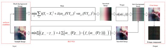
Figure 1.
Spatial dimensions push sweep hyperspectral imaging system noise removal method.
2.2. Scenario-Based Noise Removal
2.2.1. WLS Algorithm
The WLS [34] algorithm is a kind of edge-preserving filter. The purpose of this algorithm proposed in this paper is that the algorithm based on bilateral filtering cannot extract good details on a multi-scale level, and there may be artifacts, but the edge part is as good as possible. The goal of filtering is to get as close to the original image as possible, retain the edge information of the strong gradient to the greatest extent, and smooth the edge information of the small gradient. Assign the initial, undenoised image as , and the smoothed result image as . The optimization target will be determined by Formula (2).
represents the pixel position, and , represents the horizontal and vertical gradient of the output image at . Weights and are defined as follows:
2.2.2. BLF-WLS Model
The bilateral function is also known as the “edge preserving” filter because of its ability to preserve the image’s edge information. Maintaining as much of the sample picture’s edge information as possible is a key objective of image denoising because, due to the peculiarities of the samples in pathological hyperspectral images, biometric traits can still be recovered at the image’s edge. Our proposed BLF-WLS model is to embed the bilateral filter function as a weight into the weighted least squares model, so that the image can achieve the purpose of preserving edge information to a greater extent. The distinctive attribute of the BLF-WLS filtering model is that the edge information is kept as the optimization objective to maximize the retention of the edge biometric data. The BLF-WLS model is innovative in that it incorporates picture bilateral filtering results as weights into WLS optimization objectives. This is carried out in an effort to preserve as much of the edge information of medical tumor images as possible, since edge biometric traits frequently serve as a crucial point of reference for the precision of medical image diagnosis. The BLF-WLS model is shown in Formula (4):
—Input Image
—Output Image
, —Weighted value
, —Image gradient
represents the pixel position, , represent the original image and the output image, respectively, and the matrix representation of optimization objectives is shown as (5).
The image size is . Let us introduce a variable ; then, is a scalar representing the total number of pixels in the image. A diagonal matrix where and are , and together is the matrix representation of the discrete difference operator, and represents the weight of the bilateral operator. By setting the optimization goal, the gradient is 0, and the equation can be obtained as follows:
In the formula, ; as for the gradient design of weights, we did not use the logarithmic brightness of WLS algorithm, but the gradient of the original image, which has been proven to achieve a smoother effect more quickly. The weight design is as follows:
2.3. Reference Dark Background Correction
The reference dark background image refers to the instrument’s response output value when there is no light input. This value allows the spatial dimensional push sweep hyperspectral imaging system’s instrument fixed-mode noise component () to be calculated and separated. Denoising is then accomplished by removing the fringe component from the noisy image. Instrument fixed-mode noise is caused by the imaging principle of the spatial dimensional push sweep hyperspectral imaging system, and has a certain regularity. It must be removed before calculating the reflectance of tumor hyperspectral images; otherwise, it will not only affect the subjective visual effect of images, but also lead to deviations in the reflectance of biological tissues, affecting the subsequent diagnosis and classification work. In this paper, the law of the fixed-mode noise of the instrument is found through a lot of experiments and calculations, and the fixed-mode noise of the instrument is eliminated according to this law.
The sample image is captured simultaneously with the reference dark background image, which is consistent with the hyperspectral image in both the spatial and spectral dimensions. Since the varied acquisition environment will also affect the detector’s non-uniformity error, both the sample picture and the dark background image must be acquired simultaneously. Separating the edge and fringe noise of the reference image as much as possible is essential for removing non-uniform fringe noise based on the reference. Many papers have been published on the removal technology of edge extraction [14,33]. These methods usually adopt a threshold to distinguish between edge and fringe noise in the image to avoid edge blurring. However, this method incorrectly removes the weak edges of the image and preserves the strong fringe noise. WLS [34] is a good edge-preserving picture filtering and denoising technique. We smooth the reference dark background picture using the WLS algorithm, then subtract it from the original dark background image to obtain the reference dark background image’s edge component in order to more effectively separate the edges of the reference dark background image. The algorithm for removing instrument fixed-mode noise () is shown in Formula (8):
where is the new image after denoising, is the image after BLF-WLS smoothing, is the reference dark background image acquired synchronously, is called the weighting coefficient, and the specific calculation is shown in Formula (9). is the mean value of dark background data calculated by the band.
Among them, refers to the weighted least square filtering of the reference dark background image. The purpose of this step is to retain the edge value of the reference image to the greatest extent, and then subtract the value of the dark background image to obtain the edge value of the reference dark background image, and then average the value of the space and spectral dimension respectively, and, finally, obtain the weighted coefficient .
3. Experiment
3.1. Hyperspectral Brain Tumor Tissue Image Acquisition
All of the datasets of hyperspectral brain tumor tissue images are actual experimental data that were gathered in conjunction with The Second Affiliated Hospital of the Fourth Military Medical University (Tangdu Hospital). In order to obtain hyperspectral brain tumor tissue images with a spectral dimension of 258 and a spatial dimension of 700 × 600, the surgically excised tumor tissues were photographed using the spatial dimensional push scan hyperspectral imaging technology that we created. Consequently, each sample image has a data size of 700 × 600 × 258. When we obtained the sample image, we also collected a dark background image that was the same size. Typically, when a brain tumor is removed, normal brain tissue is also present in addition to the malignant tissue. We currently have 39 HSI datasets of brain tumor images from 15 distinct patients (still being collected continuously). Table 1 lists the specifications of the employed hyperspectral imaging system, and Figure 2 displays an illustration of the acquisition procedure. The specific practice is to obtain hyperspectral images of fresh brain tissue after the micromagnification of fresh brain tissue specimens cut by doctors during surgery by the spatial dimensional thru-scan hyperspectral imaging system developed by our research group, and the light source used for irradiation is a halogen light source. In order to facilitate observation, 630.25 nm (band 105), 518.05 nm (band 56), and 480.17 nm (band 39) were selected as red, green, and blue three-channel synthetic pseudo-color images.

Table 1.
Instrument parameters.
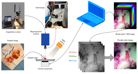
Figure 2.
Spatial dimensional push sweep hyperspectral brain tumor image acquisition system.
3.2. Denoised Image
The gathered images of brain tumors were all undergoing an attack from relatively strong non-uniform noise. We gathered four tumor images taken at various times, together with their corresponding reference dark background images, to examine the efficacy of the denoising method. Data1 through Data4 refer to the four images in the sequence of collecting time. The difference between the before and after correction is assessed using subjective evaluation criteria and an objective evaluation index of picture denoising without reference in accordance with the non-uniform strip noise removal method suggested in this paper.
The hyperspectral image of the original brain tumor is in Figure 3. It is clear that the original image typically contains non-uniform fringe noise that permeates the entire piece of data and travels along the entire band in the same direction. The center band’s fringe components are fewer, the fringe components of the other bands vary, and the front and back bands are significantly impacted by fringe noise. Figure 4 shows the image following the proposed way of removal. As can be observed, there is less loss of image detail and the non-uniform fringe noise disappears.
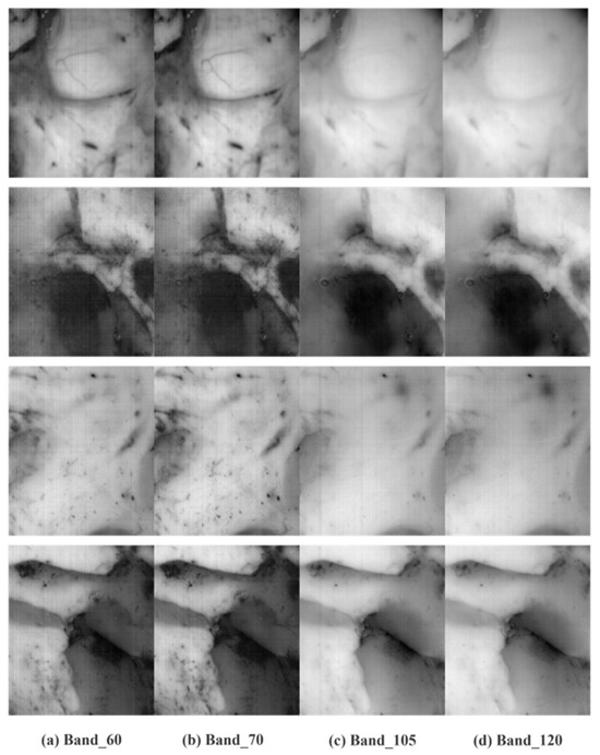
Figure 3.
Hyperspectral image of the original brain tumor.
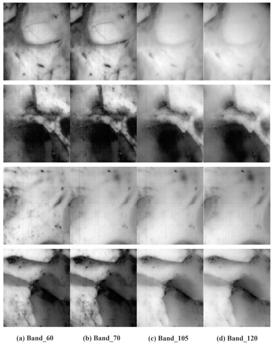
Figure 4.
Denoised hyperspectral image of brain tumor.
The grayscale distribution of the original image and the denoised image are compared in Figure 5. The amount of non-uniform noise in the image is reflected in the grayscale distribution space. While the grayscale distribution of an image with noise is not smooth and has several burrs, it is smooth once the noise has been removed, and the “burr” phenomena is clearly no longer present. The experimental results show that the denoising process is more effective than other methods, and the fringe components of the original image can be separated more thoroughly.
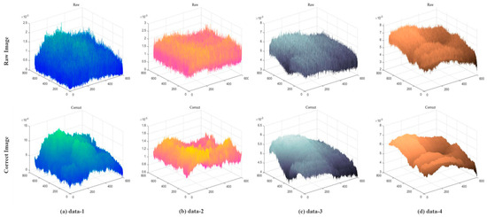
Figure 5.
Gray distribution space.
3.3. Comparative Experiment
Two traditional denoising methods (WNNM [34] and GDGIF [35]) and two neural network denoising algorithms (DNCNN [29] and ADNet [30]) were chosen for the experiment since they had better image denoising effects. The denoising effect of the algorithm is evaluated subjectively through two display modes of the single-band image and false color image. The qualitative evaluation indices include the subjective visual effect of human eyes and the column mean curve of the image. Figure 6 shows the effect of several methods on noise removal in some bands of hyperspectral images. The part specially marked is for the biological detail characteristics of tumor hyperspectral images, which plays an important role in the subsequent image processing. Therefore, cleaner noise removal and clearer details result in the best experimental results being obtained.
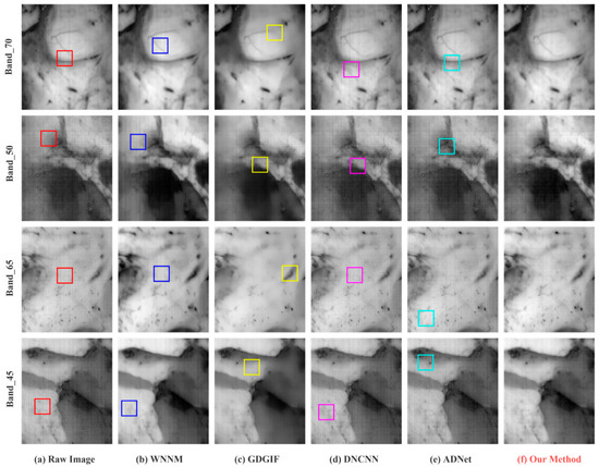
Figure 6.
Comparison of single-band images.
The experiment selected different single-band images of tumor hyperspectral images, which are important reference bands for the classification and diagnosis of subsequent tumor hyperspectral images, and some details are biological tissues or biological tissue boundaries with obvious characteristics. The four original band pictures of the images all exhibit rather significant fringe noise, as can be observed. Although the two conventional techniques have the same effect of eliminating fringe noise, they both suffer from image distortion due to excessive edge smoothing. The fringe noise after removal is still severe even if the two neural networks’ denoised images are clean and maintain the highest amount of visual information. It is evident that the separation of the fringe components is incomplete. The approach presented in this paper can successfully achieve denoising while effectively separating the fringe components.
In order to better display the denoising effect, 630.25 nm (band 105), 518.05 nm (band 56), and 480.17 nm (band 39) were selected in the experiment to synthesize pseudo-color images. Figure 7 and Figure 8 shows the denoising effect of each method and the details of the images before and after denoising.
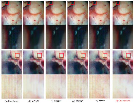
Figure 7.
Comparison of the denoising results and details in Data1 and Data2.
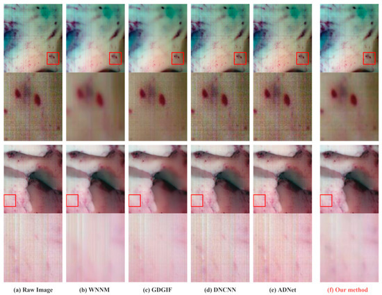
Figure 8.
Comparison of the denoising results and details in Data3 and Data4.
As can be observed, the standard filter denoising method leaves some noise in some areas of the image while being overly smooth in others, causing artifacts to form at the edges of the image. The removal of noise by a neural network do not show a significant contribution, and it may potentially add new fringe noise from the subjective influence of human vision. The detailed part specially marked includes the blood vessels of brain tissue, the boundary between tumor and normal tissue, and the gray matter of the brain, which are important references for tumor hyperspectral diagnosis methods. Therefore, the denoising effect of this part is directly related to the accuracy of the diagnostic results. The method suggested in this work may successfully eliminate non-uniform fringe noise while maintaining the image edge features, as can be convincingly demonstrated in the sections that follow.
3.4. Column Value
When removing non-uniform fringes from hyperspectral images using the moment matching approach, the column mean value is frequently employed as a crucial reference index. The precise procedure is adjusting each column’s means to the reference column’s mean and standard deviation. Since the true column mean value of the image cannot be reflected, the adjusted column mean value curve of the image is roughly a straight line, which alters the actual spectral distribution of the image. In order to assess the degree of spectral distribution retention of the denoised image, this study uses the column mean curve as a subjective evaluation index and compares it to the column mean curve of the original image.
The mean curve of the original noise-filled image column is frequently too rough, with several sharp points and extraneous peaks and valleys that complicate feature extraction and classification tasks and reduce processing accuracy. Therefore, the main objective of removing non-uniform noise is to remove this extra sharpness, making the curve as smooth as possible while maintaining the original trend, and the secondary objective is to avoid over-smoothing that would result in the loss of the curve’s details. The reflectivity value must not deviate too much from the original image in order to accomplish the aforementioned goals. Since medical hyperspectral images have dozens or even hundreds of bands, a single column mean curve for a single-band image can only reflect the non-uniform band noise removal results of a single image. In order to reflect the denoising effect of different non-uniform strip noise removal algorithms on all band images, in the experiment, the spectral dimension average of the column mean values of all bands may accurately indicate the influence of all bands’ adjustment. Figure 9 shows the comparison of the mean column mean curve before and after denoising for the whole band.
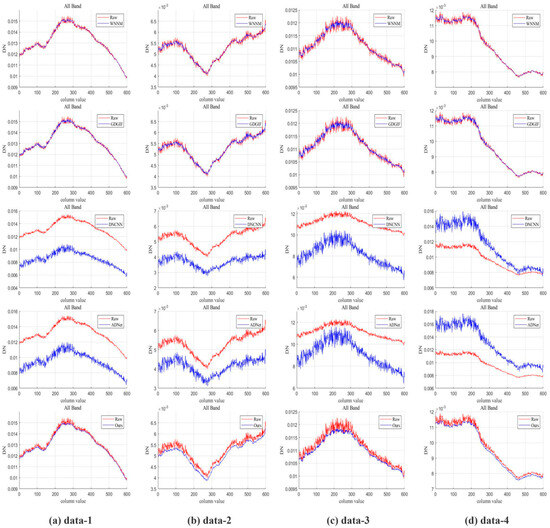
Figure 9.
Column mean curve.
The image column mean curves that have been denoised by all approaches are smoother than the original image column mean curves, and the classical denoising method is more effective than the neural network denoising method. According to the analysis, the denoising effect is not immediately apparent because there are not enough distinct reference images for the network to learn from. While the column mean distribution curve is smoothed using the conventional filtering and denoising method, some prominent feature values from the original image are also removed at the same time as the smoothing, which results in the loss of image information. Compared with the original image column mean curve, the image column mean curve after denoising by our method fits the original image column mean curve to the greatest extent, and the actual spectral distribution is best preserved.
The above subjective visual effects of human eyes directly reflect the effectiveness of non-uniform banding noise removal, thus demonstrating the rationality of the method proposed in this paper for the removal of non-uniform banding noise in the push sweep tumor hyperspectral imaging system. Our goal is to establish a dataset of brain tissue hyperspectral images, and this method will continue to be used in the subsequent images collected.
3.5. Objective Evaluation Index
The typical denoising evaluation index cannot be used in this experiment since it is based on real brain tumor tissue image data that were not obtained with a clean hyperspectral image serving as the reference image. It is believed that the universal evaluation index can be utilized as a comparison for evaluating non-reference images for denoising. The objective evaluation indicators for assessing picture quality are the NR [36] and ICV [36] coefficients. To find out if an image has fringe noise, the statistical properties of the image data are examined. Thus, in order to assess the intensity of non-uniform noise, the average noise reduction coefficient (MNR) and average inverse anomaly coefficient (MICV) are utilized in this work.
(1) MICV
The calculation formula of MICV is shown as (10):
The specific calculation method is to select a uniform image region on the removed image, calculate the mean and standard deviation of the region, respectively, and then average the calculated results in the whole band to obtain the value. The size of the image region selected in this experiment is . The larger the MICV value, the better the strip noise removal effect. The MICV calculation of the image after denoising by this method and other methods is shown in Table 2.
Table 2.
Comparison of MICV values.
(2) MNR
The NR index reflects the strip noise removal level of the image, and the formula for calculating NR is as follows:
where represents the average power spectrum of the undenoised original image, and represents the average power spectrum of the fringe noise. The larger the value of the MNR index, the stronger the denoising ability of the algorithm. We regard the single-band hyperspectral images as different images, calculate the NR value of each image, and then perform the full-band average to reflect the banding noise removal capability of the full-band hyperspectral images, and obtain the MNR calculation formula:
Both MICV and MNR indicators reflect the noise component of the image by analyzing the rules and characteristics of the data. Through a mathematical analysis, it can be seen that, the cleaner the image, the higher the value of MICV and MNR. The data in Table 3 show that the method proposed in this paper achieves a high score in the evaluation index without reference, which proves that the denoising method proposed in this paper can effectively remove the non-uniform noise of the spatial dimensional push sweep hyperspectral imaging system. In order to remove the non-uniform noise in the subsequent data collection, the approach will continue to be applied.
Table 3.
Comparison of MNR values.
4. Discussion
Non-reference hyperspectral image denoising is an important branch in the research field of hyperspectral image denoising. Due to the limitation of the imaging equipment, it is difficult to obtain clear and noiseless hyperspectral images. Most of the current denoising methods analyze the possible universal laws of images from the perspective of mathematical statistics, and regard the parts that violate the rules as noise, with a high computational complexity and weak generalization ability. In addition, the banding noise caused by different imaging modes of hyperspectral images is also different. Therefore, tracing back to the source, starting from the imaging system itself, and analyzing the reason of instrument noise can result in a better noise reduction effect.
The lack of noiseless reference images for comparison makes it difficult to conduct research on non-reference hyperspectral image denoising methods because the data that are acquired typically have non-uniform noise. There are various causes of noise production due to the variances between various imaging systems. The reference image in the spatial dimensional push sweep hyperspectral imaging system is the response output (dark background image), which has a good removal effect on the fixed-mode noise. The approach can be considered to remove the non-uniform fringe noise of the spatial dimensional push sweep hyperspectral imaging system, as demonstrated by the denoising index of no reference picture, which indicates that the sample image removed by the dark background image irradiated by no light source has good image quality. A possible limitation is that the non-signal input response output that is currently obtained does not account for temperature changes in the detector. Second, further research is necessary to determine whether variations in the detecting pixel positions across various imaging systems have an impact on the computation of correction factors. Secondly, it is necessary to confirm that the proposed approach is universal for more hyperspectral imaging equipment. As for the random signal noise caused by the imaging process, the filtering method is effective, but it will bring a decline in image quality, although it does not affect the subsequent data processing work, but the visual effect of the human eye changes. Therefore, for the removal of this part of noise, more accurate algorithms need to be explored to better balance the noise removal and visual effects.
5. Conclusions
In this paper, a method for removing non-uniform band noise in the hyperspectral imaging system is proposed in order to solve the noise problem in hyperspectral brain tumor images collected in real scenes. The proposed strategy of extracting edge information from a dark background image can the calculate correction factor more accurately and reduce the fixed-mode noise effectively. At the same time, the bilateral filter embedded least squares filter (BLF-WLS) algorithm proposed in this paper can remove the fringe noise and retain the image details well, avoiding the blur and detail loss that may be caused by the traditional denoising method. The experimental results show that the proposed method can reduce the non-uniform noise to a certain extent and maintain the image features well. By using subjective and objective evaluation indices, and comparing it with other denoising techniques, the experimental results show that the proposed method has certain advantages in the denoising effect and image detail retention. Despite the long runtime of the method, future work will focus on optimizing the smoothing algorithm to improve computational efficiency, while there are plans to extend the technique to more hyperspectral brain tumor images to further validate its effect and universality.
Author Contributions
Conceptualization, J.Y.; Software, J.Y. and M.Q.; Validation, J.Y. and C.T.; Formal analysis, C.T.; Investigation, J.Y.; Data curation, Y.W.; Writing—original draft, J.Y.; Writing—review & editing, J.Y. and C.T.; Supervision, J.D.; Project administration, Z.Z. and B.H.; Funding acquisition, Z.Z. and B.H. All authors have read and agreed to the published version of the manuscript.
Funding
This study was granted by the project of “Research on automatic hyperspectral pathology diagnosis technology” (Project No. Y855W11213) supported by the Key Laboratory Foundation of Chinese Academy of Sciences, the project of “Research on microscopic hyperspectral imaging technology” (Project No. Y839S11) supported by the Key Laboratory of Biomedical Spectroscopy of Xi’an, and the Open Research Fund for development of high-end scientific instruments and core components of the Center for Shared Technologies and Facilities, XIOPM, CAS (Project No. SJZ1-202406004).
Institutional Review Board Statement
Not applicable.
Informed Consent Statement
Not applicable.
Data Availability Statement
The data will be made available by the corresponding author upon reasonable request.
Conflicts of Interest
The authors declare that they have no conflicts of interest.
References
- Sato, D.; Takamatsu, T.; Umezawa, M.; Kitagawa, Y.; Maeda, K.; Hosokawa, N.; Okubo, K.; Kamimura, M.; Kadota, T.; Akimoto, T.; et al. Author Correction: Distinction of surgically resected gastrointestinal stromal tumor by near-infrared hyperspectral imaging. Sci. Rep. 2021, 11, 19030. [Google Scholar] [CrossRef] [PubMed]
- Hu, B.; Du, J.; Zhang, Z.; Wang, Q. Tumor tissue classification based on micro-hyperspectral technology and deep learning. Biomed. Opt. Express 2019, 10, 6370–6389. [Google Scholar] [CrossRef] [PubMed]
- Hao, Q.; Pei, Y.; Zhou, R.; Sun, B.; Sun, J.; Li, S.; Kang, X. Fusing Multiple Deep Models for In Vivo Human Brain Hyperspectral Image Classification to Identify Glioblastoma Tumor. IEEE Trans. Instrum. Meas. 2021, 70, 4007314. [Google Scholar] [CrossRef]
- Räsänen, J.; Salmivuori, M.; Pölönen, I.; Grönroos, M.; Neittaanmäki, N. Hyperspectral Imaging Reveals Spectral Differences and Can Distinguish Malignant Melanoma from Pigmented Basal Cell Carcinomas: A Pilot Study. Acta Derm.-Venereol. 2021, 101, adv00405. [Google Scholar] [CrossRef]
- Cooney, G.S.; Barberio, M.; Diana, M.; Sucher, R.; Chalopin, C.; Köhler, H. Comparison of spectral characteristics in human and pig biliary system with hyperspectral imaging (HSI). Curr. Dir. Biomed. Eng. 2020, 6, 20200012. [Google Scholar] [CrossRef]
- Bilal, A.; Liu, X.; Shafiq, M.; Ahmed, Z.; Long, H. NIMEQ-SACNet: A novel self-attention precision medicine model for vision-threatening diabetic retinopathy using image data. Comput. Biol. Med. 2024, 171, 108099. [Google Scholar] [CrossRef]
- Bilal, A.; Imran, A.; Baig, T.I.; Liu, X.; Long, H.; Alzahrani, A.; Shafiq, M. Improved Support Vector Machine based on CNN-SVD for vision-threatening diabetic retinopathy detection and classification. PLoS ONE 2024, 19, e0295951. [Google Scholar] [CrossRef]
- Ortega, S.; Fabelo, H.; Iakovidis, D.K.; Koulaouzidis, A.; Callico, G.M. Use of hyperspectral/multispectral imaging in gastroenterology: Shedding some–different–light into the dark. J. Clin. Med. 2019, 8, 36. [Google Scholar] [CrossRef] [PubMed]
- Halicek, M.; Little, J.V.; Chen, A.Y.; Fei, B. Multiparametric radiomics for predicting the aggressiveness of papillary thyroid carcinoma using hyperspectral images. In Proceedings of the Medical Imaging: Computer-Aided Diagnosis, Online, 15–20 February 2021; p. 1159728. [Google Scholar]
- Kuang, X.; Sui, X.; Chen, Q.; Gu, G. Single Infrared Image Stripe Noise Removal Using Deep Convolutional Networks. IEEE Photonics J. 2017, 9, 3900913. [Google Scholar] [CrossRef]
- Wu, B.; Liu, C.; Xu, R.; He, Z.; Liu, B.; Chen, W.; Zhang, Q. A Target-Based Non-Uniformity Self-Correction Method for Infrared Push-Broom Hyperspectral Sensors. Remote Sens. 2023, 15, 1186. [Google Scholar] [CrossRef]
- Acito, N.; Diani, M.; Corsini, G. Subspace-based striping noise reduction in hyperspectral images. IEEE Trans. Geosci. Remote Sens. 2011, 49, 1325–1342. [Google Scholar] [CrossRef]
- Arslan, Y.; Oguz, F.; Besikci, C. Extended wavelength SWIR InGaAs focal plane array: Characteristics and limitations. Infrared Phys. Technol. 2015, 70, 134–137. [Google Scholar] [CrossRef]
- Naratanan, B.; Hardie, R.C.; Muse, R.A. Scene-based nonuniformity correction technique that exploits knowledge of the focal-plane array readout architecture. Appl. Opt. 2005, 44, 3482–3491. [Google Scholar] [CrossRef] [PubMed]
- Gadallah, F.L.; Csillag, F.; Smith, E.J.M. Destriping multisensor imagery with moment matching. Int. J. Remote Sens. 2000, 21, 2505–2511. [Google Scholar] [CrossRef]
- Liu, L.; Chen, Y. Hyperspectral image restoration for stripe noise removal using low-rank matrix factorization. Pattern Recognit. 2021, 115, 107907. [Google Scholar] [CrossRef]
- Peng, C.; Zhang, J.; Zhao, Y.; Li, H. Hyperspectral Image Denoising Using Nonconvex Local Low-Rank and Sparse Separation With Spatial–Spectral Total Variation Regularization. IEEE Trans. Geosci. Remote Sens. 2022, 60, 1–17. [Google Scholar] [CrossRef]
- Li, D.; Chu, D.; Guan, X.; He, W.; Shen, H. Adaptive Regularized Low-Rank Tensor Decomposition for Hyperspectral Image Denoising and Destriping. IEEE Trans. Geosci. Remote Sens. 2024, 62, 5513917. [Google Scholar] [CrossRef]
- Wang, Z.C. Research on a Bilateral Filtering Based Image Denoising Algorithm for Nightly Infrared Monitoring Images. In Proceedings of the 3rd International Conference on Computer Science and Service System (CSSS), Bangkok, Thailand, 13–15 June 2014; pp. 199–203. [Google Scholar] [CrossRef]
- Li, K.; Zhong, F.; Sun, L. Hyperspectral Image Denoising Based on Multi-Resolution Gated Network with Wavelet Transform. In Proceedings of the 2022 3rd International Conference on Computer Vision, Image and Deep Learning & International Conference on Computer Engineering and Applications (CVIDL & ICCEA), Changchun, China, 20–22 May 2022; pp. 637–642. [Google Scholar] [CrossRef]
- Haar, D.; Zhang, L.; Wang, Y.; Chen, F. Haar Nuclear Norms with Applications to Remote Sensing Imagery Restoration. Remote Sens. 2023, 15, 1234–1249. [Google Scholar]
- Zhang, X.; Li, Y. A new wavelet-based denoising approach for hyperspectral image restoration under mixed noise conditions. Remote Sens. 2021, 13, 2459. [Google Scholar]
- Liu, Y.; Li, W. FIR-based noise suppression method for hyperspectral image denoising. Remote Sens. 2022, 14, 2354. [Google Scholar] [CrossRef]
- Chen, J.; Shao, Y.; Guo, H.; Wang, W.; Zhu, B. Destriping CMODIS data by power filtering. IEEE Trans. Geosci. Remote Sens. 2003, 41, 2119–2124. [Google Scholar] [CrossRef]
- Chen, B.; Feng, X.; Wu, R.; Guo, Q.; Wang, X.; Ge, S. Adaptive wavelet filter with edge compensation for remote sensing image denoising. IEEE Access 2019, 7, 91966–91979. [Google Scholar] [CrossRef]
- Wang, E.; Jiang, P.; Hou, X.; Zhu, Y.; Peng, L. Infrared stripe correction algorithm based on wavelet analysis and gradient equalization. Appl. Sci. 2019, 9, 1993. [Google Scholar] [CrossRef]
- Guan, J.; Lai, R.; Xiong, A. Wavelet deep neural network for stripe noise removal. IEEE Access 2019, 7, 44544–44554. [Google Scholar] [CrossRef]
- Chang, Y.; Yan, L.; Liu, L.; Fang, H.; Zhong, S. Infrared aerothermal nonuniform correction via deep multiscale residual network. IEEE Geosci. Remote Sens. Lett. 2019, 16, 1120–1124. [Google Scholar] [CrossRef]
- Zhang, K.; Zuo, W.; Chen, Y.; Meng, D.; Zhang, L. Beyond a Gaussian denoiser: Residual learning of deep CNN for image denoising. IEEE Trans. Image Process. 2017, 26, 3142–3155. [Google Scholar] [CrossRef] [PubMed]
- Tian, C.; Xu, Y.; Li, Z.; Zuo, W.; Fei, L.; Liu, H. Attention-guided CNN for image denoising. Neural Netw. 2020, 124, 117–129. [Google Scholar] [CrossRef]
- Rossi, A.; Diani, M.; Corsini, G. A comparison of deghosting techniques in adaptive nonuniformity correction for IR focal-plane array systems. In Proceedings of the Electro-Optical and Infrared Systems: Technology and Applications VII, Toulouse, France, 20–23 September 2010; p. 78340D. [Google Scholar] [CrossRef]
- Medina, O.J.; Pezoa, J.E.; Torres, S.N. A frequency domain model for the spatial fixed-pattern noise in infrared focal plane arrays. In Proceedings of the Infrared Sensors, Devices, and Applications; and Single Photon Imaging II, San Diego, CA, USA, 21–25 August 2011; p. 81550H. [Google Scholar] [CrossRef]
- Qian, W.; Chen, Q.; Gu, G.; Guan, Z. Correction method for stripe nonuniformity. Appl. Opt. 2010, 49, 1764–1773. [Google Scholar] [CrossRef]
- Farbman, Z.; Fattal, R.; Lischinski, D.; Szeliski, R. Edge-preserving decompositions for multi-scale tone and detail manipulation. ACM Trans. Graph. (TOG) 2008, 27, 1–10. [Google Scholar] [CrossRef]
- Gu, S.; Zhang, L.; Zuo, W.; Feng, X. Weighted Nuclear Norm Minimization with Application to Image Denoising. In Proceedings of the IEEE Conference on Computer Vision and Pattern Recognition, Columbus, OH, USA, 23–28 June 2014; pp. 2862–2869. [Google Scholar] [CrossRef]
- Li, Q.; Zhong, R.; Wang, Y. A Method for the Destriping of an Orbita Hyperspectral Image with Adaptive Moment Matching and Unidirectional Total Variation. Remote Sens. 2019, 11, 2098. [Google Scholar] [CrossRef]
Disclaimer/Publisher’s Note: The statements, opinions and data contained in all publications are solely those of the individual author(s) and contributor(s) and not of MDPI and/or the editor(s). MDPI and/or the editor(s) disclaim responsibility for any injury to people or property resulting from any ideas, methods, instructions or products referred to in the content. |
© 2024 by the authors. Licensee MDPI, Basel, Switzerland. This article is an open access article distributed under the terms and conditions of the Creative Commons Attribution (CC BY) license (https://creativecommons.org/licenses/by/4.0/).