Abstract
In the domain of modern manufacturing digitalization, artificial intelligence tools are increasingly employed for condition monitoring and technical diagnostics. However, the majority of existing methodologies primarily concentrate on the technical diagnosis of rotating machines, with a noticeable lack of research addressing these issues in sequential machines. In this paper, we deal with the selection of suitable vibration signal characteristics for the detection of an industrial robot’s release from its base during a handling operation. Statistical methods, including one-way ANOVA and t-tests, were used to identify the most significant features, which allowed us to isolate vibration metrics with significant predictive potential. These selected features were then used as inputs to various machine learning models to evaluate the hypothesis that these parameters can reliably indicate fastening releasing events. The results show that the optimized parameters significantly improve the detection accuracy, thus providing a reliable basis for future applications in predictive maintenance and monitoring. The findings represent an advance in robotic condition monitoring, providing a structured approach to feature selection that improves the reliability of disconnection detection in automated systems with potential applicability in various industrial environments.
1. Introduction
Condition monitoring is an effective and widely used tool in modern manufacturing. It contributes to improving production productivity and reliability. Condition monitoring of a variety of industrial equipment is used today to ensure that it is possible to detect any problems in time to prevent unplanned downtime and extensive damage.
Vibrodiagnostics plays a significant role in monitoring the condition of machinery and equipment. Vibration signatures are an attractive parameter for condition monitoring as they are easily measurable and allow up-to-date information about the machine’s condition without direct intervention in the production process. By analysing vibration patterns, anomalies such as mechanical damage, misalignment, or component failures can be detected in the machine long before they develop into critical problems [1,2].
In addition to the traditional statistical methods of evaluation and processing of such signals, methods or algorithms based on artificial intelligence are also gaining popularity, as they can monitor and evaluate non-linear dependencies of the analysed parameters [3,4,5]. Lorenz et. all [5] in the study defines several key techniques that are currently used in vibration signal classification, which include Fuzzy Logic [6,7], Artificial Neural Networks [8,9,10,11,12,13], and traditional signal processing techniques [14,15,16]. Recent research in this field has also explored the application of various machine learning and AI techniques for vibration-based condition monitoring and fault diagnosis of rotating machinery [17,18,19,20,21,22].
The key advantages of these techniques include improved diagnostic accuracy, reduced analysis effort, and the ability to handle complex, nonlinear relationships in vibration data [18,19,20]. A growing trend can be seen with the implementation of models based on various machine learning principles, even in industrial cases [3,23,24,25,26].
The diversity of model architectures used is also noticeable. LSTM and recurrent neural networks have been successfully used for RUL prediction [10,27] and maintenance task scheduling [28]. Deep convolutional neural networks, in addition to the traditional visual data processing domain, have been successfully used for bearing fault detection [29,30,31], gear faults [2,32], and shaft misalignments [19].
Researchers have also explored the integration of AI-based methods with traditional vibration analysis techniques, such as time-frequency analysis to enhance the diagnosis of rotating machinery under variable speed conditions [33,34]. These hybrid approaches have improved performance in extracting relevant features and identifying fault signatures [33,34].
However, there are still some gaps and challenges in this area of research. Data-driven models typically rely on signal processing, which demands increased computational capacity and can pose significant challenges in real manufacturing environments. Moreover, it is essential to investigate the integration of machine learning with various data sources and domain-specific knowledge to improve the performance and reliability of these techniques [5,26]. Furthermore, the interpretability and explainability of AI-based vibration diagnosis methods is an area that requires further research [18,20]. In addition, a more comprehensive investigation is necessary to evaluate the robustness of these techniques in response to environmental and operational changes, as well as to ascertain their applicability to a broader range of rotating machine types [20,22,26].
2. Motivation
As shown above, vibrodiagnostics and condition monitoring are closely related and represent an important and relevant domain of interest for science and practical application. However, the primary research is dedicated to the field of rotating machinery and components, for which there are validated methods of vibration signal processing in the time domain, frequency domain, and time-frequency domain [2].
At the same time, it is evident that studies focusing on the vibrodiagnostics of sequential machines, including industrial robots, are significantly fewer than those addressing the vibrodiagnostics of rotational components. In the case of industrial robotics-related research, it is possible to see examples of successful applications of combined approaches based on deep neural networks for anomaly detection [35] and models used for audio-based fault detection [36]. There are also methods based on optical flow processing for detecting robot arm motion errors [37] and classification models based on the motion parameters of the joints of the industrial robot arm [38]. In previous research, we have also validated the ability of the LSTM neural network to classify the robot motion speed based on the vibration signal obtained from the MEMS accelerometer [39]. Within the broader field of vibrodiagnostics, industrial robot vibrodiagnostics also face similar challenges. These include difficulties in interpreting the designed models, the need for signal pre-processing, and complicated integration into real industrial environments. This is often compounded by the computational complexity and the inherently complex nature of operations performed under unstable conditions, such as load variations and variations in operating speed.
In modern manufacturing, the field of application of industrial robots is much more extensive than just handling heavy products. It also includes applications requiring high precision, such as machining, measuring, precision assembly, etc. In precision applications, it is important to maintain stable values of the performance criteria of an industrial robot [40]. Therefore, early identification of changes in these parameters can prevent the occurrence of collision situations or the production of non-conforming products.
The objective of our research is to contribute to the resolution of problems associated with vibrodiagnostics, with a particular focus on industrial robots. We have focused our attention on the selection of appropriate vibration signal characteristics, intending to facilitate the application of AI and ML-based models into real production environments. The selected features should be straightforward to compute, while simultaneously providing sufficient attributes to enable the detection of anomalies in the operation of an industrial robot using machine learning and artificial intelligence models.
Based on the above, in the present paper, we consider the selection of the most effective metrics and properties of vibration signals that could be used in a follow-up implementation in a production environment for the detection of potential faults and predictive maintenance of industrial robots. The case study deals with the detection of the release of a FANUC industrial robot from its base during a handling operation for the application of the obtained knowledge in the predictive maintenance of sequential machines.
Based on the aforementioned, the hypothesis of the given research is that, based on the selected parameters of the vibration signal, it is possible to use the selected machine learning algorithms to detect the unfastening of the robot at its base with an accuracy of at least 95%.
3. Preparation of the Experiment
Tracking robot fastening release is crucial for ensuring production quality, preventing downtime, and improving maintenance processes. This ultimately leads to more reliable and cost-effective operations. Traditional methods of detecting robot fastening loosening often rely on manual checks or basic feedback from sensors.
However, recent advances in machine learning and signal processing represent a transformative approach to this challenge. By analysing the specific parameters of vibration signals generated during robot operation, machine learning algorithms can detect even subtle changes in the robot’s fastening. In our case, the main goal of the experiment is to find out what vibration signal metrics can provide relevant and objective data about the robot’s fastening to its base.
3.1. Robotic Workstation and Work Cycle
The experiments took place at the assembly workstation (Figure 1) in the laboratory at the Department of Automation and Production Systems, University of Žilina. The industrial robot Fanuc LR Mate 200iC was responsible for carrying out manipulation tasks within this workplace. The assembly and subsequent manipulation tasks of the industrial robot were designed to closely simulate real production process conditions.
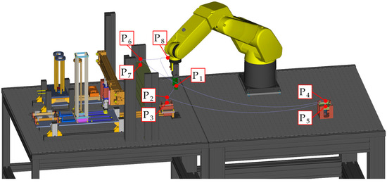
Figure 1.
Robotic workstation.
During the working cycle, the robot takes the pre-assembled products from the assembly station (Figure 1, points P2 and P3), moves them to the fixture (Figure 1, points P4, P5), and finally places them in the storage rack (Figure 1, points P6, P7, P8). In real production, cycle time plays a significant role because reducing cycle time is crucial for increasing overall productivity in the production process. For this reason, the program for the industrial robot is designed to ensure that all movements are carried out at the maximum speed of the TCP (Tool Center Point) of the robot. During the process of removing a part and inserting it into the fixture and storage rack, the robot’s end member moves at low speeds to ensure accuracy and safety. The specific values of the robot’s TCP speeds when moving between points are detailed in Table 1. The total working cycle time of the robot is 17.93 s.

Table 1.
Movement speeds of the robot’s TCP.
The Fanuc LR Mate 200iC (FANUC CORPORATION, Oshino-mura, Yamanashi Prefecture, Japan) industrial robot is fastened to the work surface using a mounting plate attached to a table made of modular profiles. The robot is fastened to the mounting plate with four M10×25 screws (torqued to 64 Nm) [41], and the plate is then clamped to the workbench using four M8×20 screws (torqued to 30 Nm) [41] and T-nuts. The clamping method is illustrated in Figure 2.
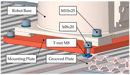
Figure 2.
Clamping method used for industrial robot.
3.2. Vibration Monitoring Sensors Description and Positioning
During the experiment, we simulated the release of the robot fastening by loosening the M8×20 screws, which secure the robot and the clamping plate to the workbench. We used Baluff BCM0002 (Balluff GmbH, Neuhausen, Germany) condition monitoring sensors for the experiment. These sensors can detect not only vibrations, but also other operational data related to the equipment or its environment, such as surface temperature, humidity, and atmospheric pressure. The essential technical specifications of the sensor used can be found in Table 2.
Table 2.
Technical characteristics for vibrations of condition monitoring sensor.
For the measurements, three sensors, which were placed on the mounting plate via a Balluff BAM03FA magnetic bracket (see Figure 3a) were used. This type of magnetic bracket is used specifically for this sensor type and the installation has been carried out according to the sensor manufacturer’s instructions. The positioning of the sensors is shown in Figure 3b. The position of the sensors was determined with a view to install them as close as possible to the object to be traced while ensuring that the accelerometer axes were aligned with the robot’s World Coordinate System (WCS).
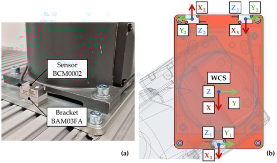
Figure 3.
Sensor clamping method (a), and placement of sensors on the clamping plate, including orientation of accelerometer axes (b).
4. Experimental Methodology
In the following section, we focus on the methodology for the experimental investigation of release detection for industrial robots during manipulation operations. This research methodology comprises several interdependent stages, each described in detail in the individual subsections. These range from the procedures for data collection and pre-processing to the selection of the crucial characteristics of the vibration signal for subsequent use in the implementation of the chosen machine learning techniques.
The primary objective of this chapter is to present a comprehensive framework for industrial robot unfastening detection that combines advanced signal processing technologies and artificial intelligence methods.
4.1. Data Gathering
Selected industrial condition monitoring sensors offer the possibility of sensing a number of various parameters that need to be configured via a web-based interface. In the presented research, we are dealing with an industrial robot, which belongs to the class of sequential machines, along with presses, pneumatic linear actuators, and linear drives. For sequential machines, three vibration monitoring profiles are available. These profiles vary according to the speed of the machine. In the case of our research, in this context, the profile was set to sense at very fast process speeds. The sensor calculates the RMS and peak-to-peak values of the vibration velocity for the three axes within the configured time window of the vibration module.
Both methods have their advantages and disadvantages and specific areas of application. The RMS method has proven to be more effective in monitoring the long-term effects of vibration on various equipment and structures. This method provides a comprehensive overview of the total vibration intensity, which is crucial for failure prediction. For this research, we decided to use the peak-to-peak (P-P) method. This represents the measurement from the minimum peak to the maximum peak of the signal (Figure 4). An increase in this value may indicate the occurrence of spikes or faults. Measuring this metric is useful in applications where it is important to know the maximum vibration amplitude, which aids in real-time fault detection [42].
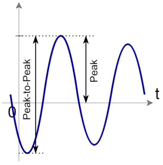
Figure 4.
Peak-to-peak measurement.
The vibration velocity data is collected by the IO-Link hub, which subsequently communicates with the PC using Matlab script. One BCM sensor cyclically transmits four parameters at the same time (20 bytes of real-time data) through the IO-Link interface. These are divided into five slots, each with 4 bytes. The first four slots contain float32 numbers, which contain information about the P-P values of the vibration velocity for a certain set time window (20 ms). The next process is to decode the values and store them in a .csv file for post-processing. The experimental data were collected from three BCM sensors. Each sensor captures peak-to-peak velocity values in three axes (X, Y, and Z axes).
Abnormal robot operation data includes vibration patterns in cases where the robot attachment to the base is loosened due to multiple forces in the operating process. This condition was simulated by manually loosening all screws after 6 h of operation. Therefore, in the case of our research, all data collected before the loosening moment is considered normal data. Since the fact that the exact moment when the base started loosening is clearly defined, we can consider that all data after this event correspond to anomalous conditions.
4.2. Data Preparation
Data preprocessing is essential for improving the quality and performance of machine learning models because it ensures that the input data is in an optimized format for the algorithms, thereby minimizing errors and maximizing prediction accuracy. In general, data preprocessing includes such steps as normalization, removal of missing values and duplicate records, correction or removal of defective data that does not indicate an error in the operation of the device but errors in the data collection process, etc. The proposed methods of preparing the data obtained in the experiments will be described in more detail below.
4.2.1. Data Preprocessing
The data collected for the experiment represent the P-P values of the acceleration in the X, Y, and Z axes for each of the three sensors that are located on the robot’s base. The dataset includes 10 input parameters: a timestamp and nine records of the recorded vibrations (in the X, Y, and Z axes for the 3 sensors). In addition, the moment, when the robot’s fastening on the pedestal was released is also known (after 6 h of continuous operation).
The data set was divided into normal operation data and data corresponding to abnormal conditions. The following data were processed into sequences. Each sequence corresponds to one robot operating cycle. The length of one sequence is 17.93 s, which corresponds to 52 callbacks from the BCM0002 sensor. For solving the following classification task, each sequence was also labelled “Normal” if the sequence corresponds to a fault-free operation of the machine and “Anomaly” if the sequence corresponds to the operation of the robot on a loose base. Examples of a normal and abnormal sequence are shown in Figure 5.
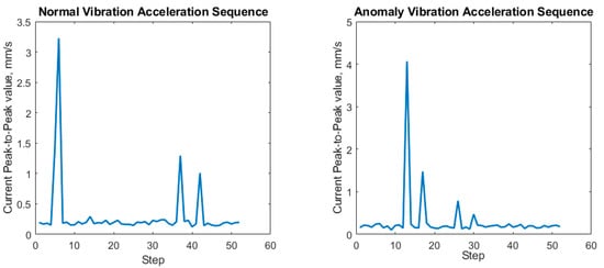
Figure 5.
Examples of normal and anomaly sequences.
Since the sensor transmits the pre-processed signal within the selected time window by the set profile, it is not necessary to use additional data processing, such as signal filtering, interpolation, or removal of invalid values.
4.2.2. Feature Extraction
Feature extraction is a crucial step in the machine learning process because it transforms the raw data into a set of relevant and meaningful attributes that better represent the underlying patterns necessary for analysis. By isolating these key features, feature extraction helps to reduce the dimensionality of the data, making it more manageable and computationally efficient for machine learning algorithms to process. In addition, effective feature extraction helps reduce the risk of overfitting when the model might otherwise tend to merely over-replicate erroneous patterns.
There are many techniques to extract features. In particular, the frequently used ones are [43]:
- Time-Domain Features—signal amplitude, zero-crossing rate, sum of squared amplitudes (signal energy), signal entropy.
- Frequency-Domain Features—Fourier Transform, Power Spectral Density (PSD), Spectral Centroid, Spectral Bandwidth.
- Time-Frequency Features—Wavelet Transform, Short-Time Fourier Transform (STFT).
- Statistical Features—Statistical measures that describe the distribution and shape of the signal data (mean, variance, skewness, kurtosis, etc.), autocorrelation.
- Other the application-specific techniques.
To extract signal features, we used the Diagnostic Feature Designer tool from Matlab software. It allows rapid feature extraction of signals using selected techniques and the subsequent selection of the most relevant features using multiple evaluation algorithms that use specific criteria to determine which features are the most effective.
As mentioned previously, a large number of criteria are defined for rotating machines and components such as gearboxes, bearings, and rotors of electric motors [5]. However, for sequential mechanisms, there is a lack of research in the relevant field. For this reason, it is difficult to predict what signal characteristics will best indicate the state of the device. At the same time, the dataset contains nine parameters, so calculating all possible properties that the software offers for all signals and their subsequent analysis would be time-consuming and computationally intensive. Therefore, we decided to use only statistical features, and for the first attempt, feature extraction was performed for one sensor (using data from all three axes).
For the sensor located at the front of the robot’s base (see Figure 3), the basic statistical features of the signal were computed. These properties can be applied to any kind of signal, including the time-synchronized average (TSA) vibration signal. Any changes in these features can indicate changes in the state of the system. The calculated features are:
- clearance factor,
- crest factor,
- impulse factor,
- kurtosis,
- mean,
- RMS,
- skewness,
- std.
Next, selecting the features that most accurately represent the predicted variable is necessary. From an initial point of view, a feature can be effective if it separates data groups with different state labels (normal and anomaly) with sufficient clarity. For an initial evaluation of the effectiveness of the feature, histograms were plotted (Figure 6) to show the separation of data between the group of normal and anomalous sequences.
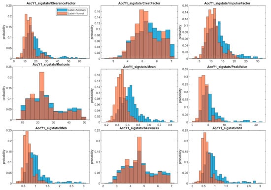
Figure 6.
Feature histograms for normal and anomaly data.
Figure 6 shows histograms representing the distribution of various statistical properties of the dataset. The width of one column in each case is chosen individually depending on the range of change in the value of a given property for a better graphical representation. From the analysis of these bar charts, it is possible to observe that even though none of the metrics show a perfect distribution of normal and abnormal sequences, it is possible to observe the following dependencies:
- ClearanceFactor, PeakFactor, Mean, Std, RMS, and PeakValue properties have the lowest overlap (shown in brown in Figure 6) between them, and a slight rightward shift in the distribution of anomalous values can be seen for each of these properties. At first glance, these properties seem to be able to describe the investigated signal more explicitly.
- In contrast, the feature factors Skewness and Kurtosis show a large rate of overlap and an almost identical distribution of data along the horizontal axis. The CrestFactor feature, while characterized by less overlap, also shows the same distribution along the horizontal axis.
It can be concluded that the most significant metrics are with high probability among the first group of features. Since the graphical representation only allows a first insight into the aspect in which each feature represents the target categorical variable, to select the right features for training machine learning models and to increase the efficiency of the training process, analysis and selection of appropriate features will be performed in the next step.
4.3. Feature Ranking Methods
Selecting relevant features for machine learning is another crucial step in developing an effective machine learning model. This means selecting only those attributes that have a significant impact on the output of the model.
After feature extraction, the experiment dataset contains nine new features for each axis of each sensor; thus, the total number of potential features for designing and training machine learning algorithms is 81 (or 27 for a single sensor). However, some of these features may be redundant, some may be correlated, and some may be irrelevant to the model. In this case, using the whole dataset for training the model may lead to an overfitting. With overfitting, the machine learning model loses the ability to generalize the patterns and characteristics that were detected in the training data, leading to low accuracy of the trained model on the new data. To avoid this, we performed simple statistical feature selection algorithms: t-test and one-way ANOVA.
4.3.1. T-Test
T-test can be applied between two classes to compare their means and conclude whether they are from the same distribution. In doing so, it is assumed that the distribution of the parameter under examination is normal. A high t-test value for a given parameter indicates that the investigated parameter (feature) varies widely for each class and, hence, represents a suitable choice for training a machine learning classification algorithm. The computation of the T-value for each pair of parameters is according to the Formula (1), where and are the means of the two groups being compared, and are the pooled standard errors of the two groups, and and are the number of observations in each of the groups.
When selecting appropriate features using a t-test, the null hypothesis and alternative hypothesis are critical in determining the significance of each feature with the target variable.
The null hypothesis usually assumes that there is no significant difference in the mean values of an element between different groups of the target variable. That means that the attribute provides no discriminating power between groups and any observed differences in means are caused by random chance. In the present research, the null hypothesis is established as follows:
H0:
There is no significant difference between anomalous and normal data for the values of the investigated feature.
The alternative hypothesis suggests that there is a statistically significant difference in the mean values of the feature between the groups. This indicates that this feature could potentially be useful for distinguishing between classes and should be considered for inclusion in the model. The alternative hypothesis is stated as follows:
H1:
The difference between the anomalous and normal data in the investigated feature is substantial, making it meaningful for classification tasks.
After calculating values for each parameter, the features were sorted by importance. The histograms in Figure 7 show all calculated features for each axis, sorted by importance.
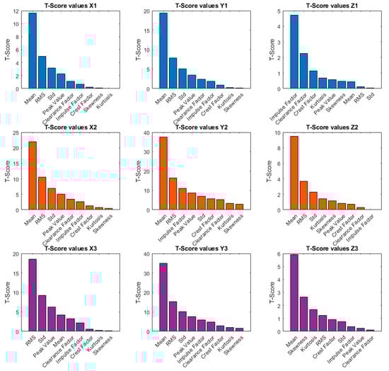
Figure 7.
T-score values for each sensor.
After the performed calculation, it is important to compare values with the defined critical value of the to decide if the null hypothesis will be rejected for the selected feature. A lower calculated than the critical value leads to the rejection of the null hypothesis, therefore supporting the alternative hypothesis. This process allows the selection of features that have a statistically significant relationship with the target variable, enhancing the predictive power of the model. The table below (Table 3) shows the parameters for which the alternative hypothesis was accepted. In the present research, the number of degrees of freedom is assumed to be , the significance level is , and the critical value of the is .
Table 3.
Accepting an alternative or null hypothesis for the specified signal features based on a t-test.
Based on the t-test, for sensor 1 for the X1 axis (Figure 7), the Mean feature has the highest , which means that it is the most significant in discriminating between classes. RMS, STD, and Peak Value also show a relatively high . For the Y1 axis, the results are similar to the case of the X1 axis: Mean has the highest . This parameter is followed by RMS and Std metrics. The Z1 axis shows a different pattern—in this case, the Impulse Factor, Clearance Factor, and Skewness parameters were shown to be the most significant factors.
For sensor 2, for the X2 and Z2 axes (Figure 7), the Mean parameter again leads with the highest , followed by the RMS and Std parameters. For the Y2 axis, the Mean parameter also leads, followed by the STD and Impulse Factor as significant features.
For sensor 3, the most significant parameter for the X3 axis (Figure 7) is RMS, followed by Std and Peak Value. For the Y3 axis, Mean, RMS, and Std lead as the most significant parameters. Mean and Skewness are the most significant parameters for the Z3 axis.
4.3.2. One-Way ANOVA
Analysis of variance is used to compare sample means for two or more classes and determine if observed differences may be due to chance or reflect true differences between classes. Like the t-test, the null hypothesis (that there is no difference between the means of the groups) and the alternative hypothesis (that at least one group is significantly different from the overall mean of the dependent variable) are established. A significant difference in the means indicates that the function has good discriminative capacity and is likely to be useful in discriminating between classes in a classification task.
One-way ANOVA was performed in the context of the present paper with the following parameters: , the significance level is , and the critical value of is . Figure 8 shows bar graphs of the for each of the characteristics under investigation.
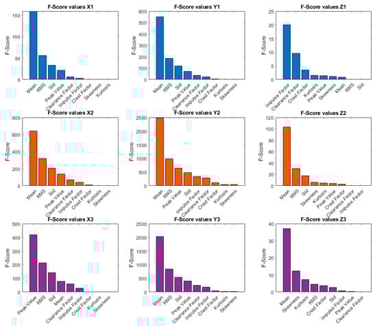
Figure 8.
F-score values for each sensor.
A higher indicates that the group means are more spread out, suggesting that a significant difference may exist between at least one pair of groups. Similar to the t-test, if the calculated for a given variable is less than a specified critical value, the null hypothesis is confirmed for that trait and the parameter is considered to have low discriminatory power. Table 4 shows for which parameters the null hypothesis was rejected, and the alternative hypothesis was accepted.
Table 4.
Accepting an alternative or null hypothesis for the specified signal features based on one-way ANOVA.
The results of the one-way ANOVA analysis for sensor 1 (Figure 8) are identical to the t-test results and again demonstrate that within the X1 axis and Y1 axis Mean, Std, and RMS are the features with the highest resolution for the anomalous and normal data. In contrast to X1 and Y1, for the Z1 axis, Impulse Factor has the highest , indicating that it is crucial for class distribution in this dataset, but RMS and Std have a very low , indicating low relevance of the given features.
For sensor 2 in all three axes (Figure 8), the Mean parameter has the highest , followed by the RMS and Std parameters for the X2 and Z2 axes, and the RMS and Peak Value parameters for the Y2 axis.
Sensor 3 differs from the standard displays, especially within the X3 axis (Figure 8). Peak Value has the highest , indicating that it is the most important feature of this data set. This is followed by RMS and Std, while Skewness and Kurtosis have minimal significance. For the Y3 axis, the dominant feature is again Mean, while for the Z3 axis dominant features are also Skewness and Kurtosis, as in the case of the t-test.
4.4. Feature Selection
After the one-way ANOVA and t-test analyses were performed, the analysis of statistical results along with the analysis of the obtained histograms were followed to select relevant features for the training of the following machine learning algorithms. The selection of the features also considered the fact that, for the potential application of the classification model in practice in terms of optimizing data processing times, it is necessary to select the same parameters for each axis.
It can be concluded that among the listed signal properties, none can be used to explicitly identify anomalies in the signal waveform from all three sensors in each axis, suggesting the need to use a set of properties to identify the errors. However, based on the above, some significant dependencies in data can be observed.
Mean is consistently one of the most important characteristics in most data sets and often shows the highest in the case of t-test and in the case of one-way ANOVA. It can also be seen in the bar graphs in Figure 7 and Figure 8 that the values of the statistical score for a given trait are much higher in most cases than the values of any other feature. RMS and Std are also often significant in distinguishing between groups of anomalous and normal data. These features are likely to be crucial for classification tasks.
Peak Value in addition to Mean, RMS, and Std, has a relatively high , suggesting that it is also a potential key feature for classification. For the above parameters, the alternative hypothesis was accepted in most cases (6 features out of 9 for t-test and 7 out of 9 for one-way ANOVA). The acceptance of the null hypothesis for Mean, Std, and RMS in the case of Z1 is likely due to the sensor location in the middle of the front face of the base of the robot and, hence, significantly less variation in the anomalous data compared to sensors that are located near the fixing screws.
After generalizing the above, we decided to use Mean, Std, RMS, and Peak Value parameters as key metrics for designing and training machine learning algorithms for the detection classification of normal and abnormal vibration sequences. The selection of the key features allowed us to reduce the dimensionality from the original 27 parameters for a single sensor (81 parameters for the whole dataset) to 12 parameters for a single sensor (36 parameters for the whole dataset). In addition, the Balluff BCM0002 sensors, when properly configured with the sensing profiles, allow direct sensing of three of the selected metrics, namely, Mean, RMS, and Std of the signal, which is also a benefit for feature implementation of the trained models.
4.5. Machine Learning Models for Unfastening Detection
For the next step, we designed several artificial neural network models and popular ensemble learning models because their classification abilities have been demonstrated in many previous studies. A brief description of the structures of the models used is given in Table 5 and Table 6.
Table 5.
Ensemble models.
Table 6.
Neural network models.
The design and training of the machine learning models were performed using Classification Learner in MATLAB software. The Classification Learner application simplifies the training of models for data classification. This tool allows rapid testing of multiple classifiers simultaneously using a comprehensive environment for exploring data, selecting features, specifying validation schemes, training models, and evaluating results.
All the proposed algorithms belong to the class of supervised learning algorithms, which require the use of a pre-labelled dataset for training and testing purposes. The data used in the present research contains two classes namely “Normal” and “Anomaly” and are divided into training data (70% of the original dataset) and test data (30% of the original dataset).
5. Detection of the Robot Mounting Release from the Base Using Machine Learning Algorithms
Detecting loose robot fasteners is key to ensuring the reliability and safety of the entire automated process. Traditional methods for detecting loose fasteners tend to rely on manual inspection or fixed rule-based systems that are error-prone and limited in adaptability. In contrast, machine learning algorithms can use large data sets to learn complex patterns related to mounting anomalies, enabling more robust and scalable detection solutions.
As mentioned, choosing key signal features reduced the total number of training parameters from 81 to 36 for the whole dataset. However, the fact that the selected metrics are the same for each sensor must be considered. Therefore, it may be irrational to design and train machine learning models using data from all three sensors.
Correct placement of the minimum required number of sensors also plays an essential role in condition monitoring. The manufacturer of the Balluff BCM0002 sensors suggests methods for sensor placement, shown in Figure 9. These methods are common for monitoring rotating components.
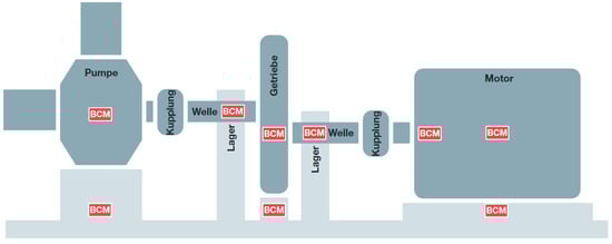
Figure 9.
Examples of placement of BCM-type sensors for correct vibration measurement [44].
However, we investigate the release detection of a sequential machine. For this reason, we decided to place one sensor in accordance with the manufacturer’s recommendation (sensor 1 in Figure 3). The two remaining sensors were placed at the locations where the most variation in attachment release is expected to occur. For the above reasons, we decided to divide experiment into two steps:
- Firstly, the selected models are trained and tested separately on data from each sensor.
- Next, for the final analysis, data from sensors that enable the models to demonstrate the highest accuracy will be utilized.
In the next section, we test designed machine learning techniques for detecting loose assembly elements in robotic assembly processes. We will use the signal features selected in the previous section for training and verification of the selected models. Our goal is to prove the main hypothesis of the current research and to establish basic concepts for future research in the field of technical diagnosis of sequential mechanisms using machine learning algorithms.
5.1. Testing Chosen Machine Learning Models for Unfastening Detection
Models that were introduced in the Section 4.5 were trained on data from each of the sensors. To avoid overfitting and to examine the accuracy of each model, a cross-validation method was chosen.
The classification results after training are shown in Table 7 and Table 8. The accuracy of all models based on sensor 1 data is significantly lower than that of sensor 2 and sensor 3, for which the accuracy is comparable and above 90%. This fact can be explained by the configuration of the workstation and the robot’s behaviour: all the tasks that the robot performs during the working cycle take place in front of the robot’s base, and thus vibrations caused by the releasing of the robot’s fastening are more visible on sensors 2 and 3, which are located at the rear part of the mounting plate (see Figure 3).
Table 7.
Ensemble model accuracy.
Table 8.
Neural network model accuracy.
For all models used, except Boosted Trees and Subspace Discriminant at a given stage, the main research hypothesis is assumed to be met using data from sensors 2 and 3 (classification accuracy is above 95%). Therefore, we excluded Boosted Trees and Subspace Discriminant models from subsequent analysis. Next, since sensors 2 and 3 differ only in their axis orientation, and the prediction results after validation on the training data are largely the same, we decided to focus only on sensor 2 for the following analysis and testing using new data.
5.2. Testing Results and Discussion
To prove that the selected machine learning algorithms can detect the robot’s releasing at the base with an accuracy of 95% or higher by using specific parameters of the vibration signal, we tested the chosen machine learning models using new data gathered from sensor 2. The test data considered a total of 590 observations, including 297 normal sequences and 293 anomaly sequences. The resulting testing accuracy is shown in Table 9, sorted by highest accuracy.
Table 9.
Tested classification accuracy.
As can be seen, all models except Subspace KNN achieved a resulting accuracy on the test data above 95%. However, the percentage accuracy shows only the number of correct predictions (both positive and negative) out of all predictions (Formula (2)). Even though the test dataset can be considered consistent since the numbers of normal and abnormal samples are almost the same, we took a closer look at the performance of the models since, in real operations, misclassification of an anomalous sequence as normal can have serious consequences.
To examine the performance of the models using the new data, we used confusion matrices compiled for the Wide Neural Network model, which was the model with the highest accuracy, and the Subspace KNN model, which proved to have the lowest percentage accuracy.
Using the confusion matrix helps to summarize the prediction results and gives an overview of how well the models perform in different classes. The confusion matrix allows a comprehensive view of the models using three more metrics, namely, recall, precision, and specificity, in addition to accuracy. Confusion matrices for the selected models are shown in Figure 10.
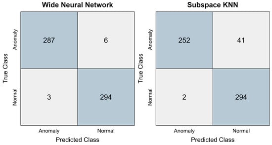
Figure 10.
Confusion matrixes for selected models.
The resulting accuracy of the model (Precision) is given by Equation (3), where TP, or true positive, refers to a sample that belongs to the class “Normal” and is correctly classified. FP, or false positive, represents the number of samples that have been classified as normal even though they represent anomalous data. This metric shows how many of the predicted positive cases were truly positive. High precision means a low rate of false positive cases [45].
Recall for the positive class shows the number of samples correctly predicted as belonging to the positive class out of all samples that truly belong to the positive class. This metric is represented by Equation (4), where FN, or false negative, refers to a sample that belongs to the normal class but is misclassified as belonging to the anomalous class [45].
Another particularly useful metric for the defined problem is specificity, which is the number of samples correctly assigned to the anomalous class out of all samples in the dataset that truly belong to the anomalous class. Specificity is calculated using Equation (5), where TN, or true negative, refers to the sample that belongs to the anomalous class and is correctly classified [45].
These metrics were calculated for all tested models. The results are presented in Table 10.
Table 10.
Calculated evaluation metrics.
As we mentioned at the beginning of the section, the Wide Neural Network (WNN) model shows significantly better accuracy (98.47%) compared to the Subspace KNN model (92.70%), indicating that the WNN is more reliable in correctly classifying both anomalies and normal sequences.
WNN has also a higher precision (98.00%), which means that it better minimizes false positives compared to Subspace KNN, which has a lower precision (87.76%). This suggests that Subspace KNN may more often mislabel normal sequences as an anomaly sequence.
Both models perform well in the recall, with Subspace KNN slightly outperforming WNN (99.32% vs. 98.99%). This indicates that both models are highly effective in detecting anomalies, with KNN being slightly better at avoiding false negatives.
In case of specificity WNN excels here with a specificity of 97.95%, which is much higher than the 86.01% for Subspace KNN. This means that the Subspace KNN model is more prone to false positives and more likely to mislabel anomalous sequences as normal.
Based on the above, the WNN model trained using the vibration signal metrics chosen in 5.3.3 performs well in accuracy, precision, and specificity, making it more reliable in detecting true anomalies and minimizing false positives. While Subspace KNN performs slightly better in recall, indicating its strength in detecting almost all true normal sequences, the model suffers from lower accuracy and specificity, indicating a higher rate of classifying anomalous samples as normal. This factor is crucial in practical implementation, as much more expense may be incurred just by incorrectly fitting anomalous data into the normal category. For this specific anomaly detection task, the WNN model appears to be a more balanced and accurate choice overall.
6. Conclusions and Feature Work
The proposed methodology was demonstrated through a case study involving the detection of a release fault in a FANUC industrial robot during handling operations. This scenario highlights the potential of our approach for improving predictive maintenance strategies, particularly for industrial robots.
In addressing a particular problem—detecting a robot’s releasing at its base—Mean, Std, RMS, and Peak Value were shown to be the best-performing signal metrics, even under the realistic conditions of manipulation tasks concerning change in robot movement speed within the technological process. Moreover, we confirmed the hypothesis of the experiment: the chosen metrics allow the detection of anomalies in the vibration signal with an accuracy of higher than 95%, and this accuracy has been achieved for several neural network models and ensemble-learning techniques.
Furthermore, to validate the hypothesis and reveal any weaknesses in the proposed models, a classification problem was solved to detect the anomaly—detection of the robot’s release during the reloading process. Based on the Mean, Std, Peak Value, and RMS metrics of the vibration signal sequences, the performance of two machine learning models, Wide Neural Network (WNN) and Subspace K-Nearest Neighbors (KNN), were compared. The evaluation was based on four key metrics: accuracy, precision, recall, and specificity. In the analysis of the results, it was shown that although accuracies above 90% can still be considered high, the amount of incorrectly captured anomalous samples plays a key role in the choice of the right AI model. In fact, in addition to reducing the overall accuracy of the model, low values of the recall and specificity metrics indicate a low discriminative ability of the model, and therefore implementation of a similar model in practice can lead to increased costs and risks in production.
By leveraging carefully chosen vibration signal properties, our approach facilitates early fault detection, minimizes unplanned downtime, and enhances the reliability of industrial robots. These metrics will play a key role in the early detection of anomalies, enabling timely maintenance interventions and minimizing machine downtime.
In our future work, we will focus on further validating the proposed models and metrics across various robotic systems and operating conditions. Additionally, the application of these techniques, aimed at developing intelligent real-time fault detection and prediction systems for industrial equipment and improving the system’s ability to generalize across different production environments, contribute to the advancement of modern manufacturing.
Author Contributions
Conceptualization, D.F.; funding acquisition, I.K. and I.Z.; investigation, D.F. and V.T.; methodology, D.F. and V.T.; project administration, I.Z. and K.T.; supervision, I.K.; visualization, T.D.; writing—original draft preparation, D.F.; writing—review and editing, V.T. and T.D. All authors have read and agreed to the published version of the manuscript.
Funding
This research was funded by Research of Implementation Methods and Means of Artificial Intelligence in Automated Quality Control Systems of Products with Volatile Quality Parameters, 1/0470/23 and Transformation and Innovation Consortium of Robotics and Automation of the Slovak Republic (Acronym Robotic), 09I02-03-V01-00010.
Institutional Review Board Statement
Not applicable.
Informed Consent Statement
Not applicable.
Data Availability Statement
The data presented in this study are available on request from the corresponding author.
Conflicts of Interest
The authors declare no conflicts of interest.
References
- Peťková, V. Teória a Aplikácia Vybraných Metód Technickej Diagnostiky; Knapíková, A., Ed.; Technická univerzita v Košiciach: Nitra, Slovakia, 2010; ISBN 978-80-553-0483-0. [Google Scholar]
- Lei, Y.; Lin, J.; Zuo, M.J.; He, Z. Condition Monitoring and Fault Diagnosis of Planetary Gearboxes: A Review. Measurement 2014, 48, 292–305. [Google Scholar] [CrossRef]
- Fink, O. Data-Driven Intelligent Predictive Maintenance of Industrial Assets. In Women in Industrial and Systems Engineering; Springer: Cham, Switzerland, 2020; pp. 589–605. [Google Scholar]
- Carvalho, T.P.; Soares, F.A.A.M.N.; Vita, R.; Francisco, R.d.P.; Basto, J.P.; Alcalá, S.G.S. A Systematic Literature Review of Machine Learning Methods Applied to Predictive Maintenance. Comput. Ind. Eng. 2019, 137, 106024. [Google Scholar] [CrossRef]
- Lorenz, A.; Siewertsen, B.; Kyhe Clemmensen, V.; Blaamann Petersen, J.; Friederich, J.; Lazarova-Molnar, S. Vibration Data Analysis for Fault Detection in Manufacturing Systems—A Systematic Literature Review. In Proceedings of the ICIEA 2022-17th IEEE Conference on Industrial Electronics and Applications, Chengdu, China, 16–19 December 2022; pp. 851–857. [Google Scholar] [CrossRef]
- Li, C.; Cerrada, M.; Cabrera, D.; Sanchez, R.V.; Pacheco, F.; Ulutagay, G.; Valente De Oliveira, J. A Comparison of Fuzzy Clustering Algorithms for Bearing Fault Diagnosis. J. Intell. Fuzzy Syst. 2018, 34, 3565–3580. [Google Scholar] [CrossRef]
- Helmi, H.; Forouzantabar, A. Rolling Bearing Fault Detection of Electric Motor Using Time Domain and Frequency Domain Features Extraction and ANFIS. IET Electr. Power Appl. 2019, 13, 662–669. [Google Scholar] [CrossRef]
- Kumar, H.S.; Srinivasa Pai, P.; Sriram, N.S.; Vijay, G.S. ANN Based Evaluation of Performance of Wavelet Transform for Condition Monitoring of Rolling Element Bearing. Procedia Eng. 2013, 64, 805–814. [Google Scholar] [CrossRef]
- Guo, X.; Chen, L.; Shen, C. Hierarchical Adaptive Deep Convolution Neural Network and Its Application to Bearing Fault Diagnosis. Measurement 2016, 93, 490–502. [Google Scholar] [CrossRef]
- Sampaio, G.S.; Vallim Filho, A.R.d.A.; da Silva, L.S.; da Silva, L.A. Prediction of Motor Failure Time Using An Artificial Neural Network. Sensors 2019, 19, 4342. [Google Scholar] [CrossRef]
- Magar, R.; Ghule, L.; Li, J.; Zhao, Y.; Farimani, A.B. FaultNet: A Deep Convolutional Neural Network for Bearing Fault Classification. IEEE Access 2021, 9, 25189–25199. [Google Scholar] [CrossRef]
- Sepulveda, N.E.; Sinha, J. Parameter Optimisation in the Vibration-Based Machine Learning Model for Accurate and Reliable Faults Diagnosis in Rotating Machines. Machines 2020, 8, 66. [Google Scholar] [CrossRef]
- Almutairi, K.M.; Sinha, J.K. Experimental Vibration Data in Fault Diagnosis: A Machine Learning Approach to Robust Classification of Rotor and Bearing Defects in Rotating Machines. Machines 2023, 11, 943. [Google Scholar] [CrossRef]
- Gilles, J. Empirical Wavelet Transform. IEEE Trans. Signal Process. 2013, 61, 3999–4010. [Google Scholar] [CrossRef]
- Tan, L.; Jiang, J. Digital Signal Processing: Fundamentals and Applications. In Digital Signal Processing: Fundamentals and Applications, 3rd ed.; Academic Press: Cambridge, MA, USA, 2019; pp. 1–903. [Google Scholar] [CrossRef]
- Liu, Z.; Zhang, L.; Carrasco, J. Vibration Analysis for Large-Scale Wind Turbine Blade Bearing Fault Detection with an Empirical Wavelet Thresholding Method. Renew. Energy 2020, 146, 99–110. [Google Scholar] [CrossRef]
- Yuan, X.; He, Y.; Wan, S.; Qiu, M.; Jiang, H. Remote Vibration Monitoring and Fault Diagnosis System of Synchronous Motor Based on Internet of Things Technology. Mob. Inf. Syst. 2021, 2021, 3456624. [Google Scholar] [CrossRef]
- Mey, O.; Neufeld, D. Explainable AI Algorithms for Vibration Data-Based Fault Detection: Use Case-Adadpted Methods and Critical Evaluation. Sensors 2022, 22, 9037. [Google Scholar] [CrossRef]
- Mey, O.; Neudeck, W.; Schneider, A.; Enge-Rosenblatt, O. Machine Learning-Based Unbalance Detection of a Rotating Shaft Using Vibration Data. In Proceedings of the IEEE International Conference on Emerging Technologies and Factory Automation, ETFA 2020, Vienna, Austria, 8–11 September 2020; pp. 1610–1617. [Google Scholar] [CrossRef]
- Toh, G.; Park, J. Review of Vibration-Based Structural Health Monitoring Using Deep Learning. Appl. Sci. 2020, 10, 1680. [Google Scholar] [CrossRef]
- Rahman, A.; Hoque, M.E.; Rashid, F.; Alam, F.; Ahmed, M.M. Health Condition Monitoring and Control of Vibrations of a Rotating System through Vibration Analysis. J. Sens. 2022, 2022, 4281596. [Google Scholar] [CrossRef]
- Tiboni, M.; Remino, C.; Bussola, R.; Amici, C. A Review on Vibration-Based Condition Monitoring of Rotating Machinery. Appl. Sci. 2022, 12, 972. [Google Scholar] [CrossRef]
- Amihai, I.; Gitzel, R.; Kotriwala, A.M.; Pareschi, D.; Subbiah, S.; Sosale, G. An Industrial Case Study Using Vibration Data and Machine Learning to Predict Asset Health. In Proceedings of the 2018 20th IEEE International Conference on Business Informatics, CBI 2018, Vienna, Austria, 11–14 July 2018; Volume 1, pp. 178–185. [Google Scholar] [CrossRef]
- Zeba, G.; Dabić, M.; Čičak, M.; Daim, T.; Yalcin, H. Technology Mining: Artificial Intelligence in Manufacturing. Technol. Forecast Soc. Chang. 2021, 171, 120971. [Google Scholar] [CrossRef]
- Baron, P.; Kočiško, M.; Hlavatá, S.; Franas, E. Vibrodiagnostics as a Predictive Maintenance Tool in the Operation of Turbo Generators of a Small Hydropower Plant. Adv. Mech. Eng. 2022, 14, 16878132221101023. [Google Scholar] [CrossRef]
- Zuth, D.; Blecha, P.; Marada, T.; Huzlik, R.; Tuma, J.; Maradova, K.; Frkal, V. Vibrodiagnostics Faults Classification for the Safety Enhancement of Industrial Machinery. Machines 2021, 9, 222. [Google Scholar] [CrossRef]
- Rivas, A.; Fraile, J.M.; Chamoso, P.; González-Briones, A.; Sittón, I.; Corchado, J.M. A Predictive Maintenance Model Using Recurrent Neural Networks. In Proceedings of the Advances in Intelligent Systems and Computing; Springer: Berlin/Heidelberg, Germany, 2020; Volume 950, pp. 261–270. [Google Scholar]
- Wu, S.J.; Gebraeel, N.; Lawley, M.A.; Yih, Y. A Neural Network Integrated Decision Support System for Condition-Based Optimal Predictive Maintenance Policy. IEEE Trans. Syst. Man Cybern. Part A Syst. Hum. 2007, 37, 226–236. [Google Scholar] [CrossRef]
- Zan, T.; Wang, H.; Wang, M.; Liu, Z.; Gao, X. Application of Multi-Dimension Input Convolutional Neural Network in Fault Diagnosis of Rolling Bearings. Appl. Sci. 2019, 9, 2690. [Google Scholar] [CrossRef]
- Kumar, P.; Hati, A.S. Deep Convolutional Neural Network Based on Adaptive Gradient Optimizer for Fault Detection in SCIM. ISA Trans. 2021, 111, 350–359. [Google Scholar] [CrossRef] [PubMed]
- Wu, C.; Jiang, P.; Ding, C.; Feng, F.; Chen, T. Intelligent Fault Diagnosis of Rotating Machinery Based on One-Dimensional Convolutional Neural Network. Comput. Ind. 2019, 108, 53–61. [Google Scholar] [CrossRef]
- Jing, L.; Zhao, M.; Li, P.; Xu, X. A Convolutional Neural Network Based Feature Learning and Fault Diagnosis Method for the Condition Monitoring of Gearbox. Measurement 2017, 111, 1–10. [Google Scholar] [CrossRef]
- Ding, C.; Huang, W.; Shen, C.; Jiang, X.; Wang, J.; Zhu, Z. Synchroextracting Frequency Synchronous Chirplet Transform for Fault Diagnosis of Rotating Machinery under Varying Speed Conditions. Struct. Health Monit. 2023, 23, 1403–1422. [Google Scholar] [CrossRef]
- Xu, Y.; Fu, C.; Hu, N.; Huang, B.; Gu, F.; Ball, A.D. A Phase Linearisation–Based Modulation Signal Bispectrum for Analysing Cyclostationary Bearing Signals. Struct. Health Monit. 2020, 20, 1231–1246. [Google Scholar] [CrossRef]
- Fathi, K.; van de Venn, H.W.; Honegger, M. Predictive Maintenance: An Autoencoder Anomaly-Based Approach for a 3 DoF Delta Robot. Sensors 2021, 21, 6979. [Google Scholar] [CrossRef]
- Olsson, E.; Funk, P.; Bengtsson, M. Fault Diagnosis of Industrial Robots Using Acoustic Signals and Case-Based Reasoning. In Lecture Notes in Computer Science (Including Subseries Lecture Notes in Artificial Intelligence and Lecture Notes in Bioinformatics); Springer: Berlin/Heidelberg, Germany, 2004; Volume 3155, pp. 686–701. [Google Scholar] [CrossRef]
- Fan, S.; Zhang, Y.; Zhang, Y.; Fang, Z. Motion Process Monitoring Using Optical Flow–Based Principal Component Analysis-Independent Component Analysis Method. Adv. Mech. Eng. 2017, 9, 1687814017733231. [Google Scholar] [CrossRef]
- Costa, M.A.; Wullt, B.; Norrlöf, M.; Gunnarsson, S. Failure Detection in Robotic Arms Using Statistical Modeling, Machine Learning and Hybrid Gradient Boosting. Measurement 2019, 146, 425–436. [Google Scholar] [CrossRef]
- Fedorova, D.; Tlach, V.; Kuric, I. Classification of Industrial Robot Movements Based on Vibration Monitoring Data Using Lstm Neural Network. In Proceedings of the Projektowanie, Badania i Eksploatacja; Rysiński, J., Ed.; Wydawnictwo Naukowe Uniwersytetu Bielsko-Bialskiego: Bielsko-Biała, Poland, 2023; pp. 169–178. [Google Scholar]
- Kuric, I.; Tlach, V.; Císar, M.; Sagová, Z.; Zajačko, I. Examination of Industrial Robot Performance Parameters Utilizing Machine Tool Diagnostic Methods. Int. J. Adv. Robot. Syst. 2020, 17, 1729881420905723. [Google Scholar] [CrossRef]
- FANUC Corporation. FANUC Robot LR Mate 200iC/ARC Mate 50iC MECHANICAL UNIT, OPERATOR’S MANUAL; B-82584EN/08; FANUC Corporation: Yamanashi, Japan, 2011. [Google Scholar]
- Igba, J.; Alemzadeh, K.; Durugbo, C.; Eiriksson, E.T. Analysing RMS and Peak Values of Vibration Signals for Condition Monitoring of Wind Turbine Gearboxes. Renew. Energy 2016, 91, 90–106. [Google Scholar] [CrossRef]
- Zhang, C.; Mousavi, A.A.; Masri, S.F.; Gholipour, G.; Yan, K.; Li, X. Vibration Feature Extraction Using Signal Processing Techniques for Structural Health Monitoring: A Review. Mech. Syst. Signal Process. 2022, 177, 109175. [Google Scholar] [CrossRef]
- Balluff GmbH. BCM R15E-002-DI00-01,5-S4 Condition Monitoring Sensor-User’s Guide; Balluff GmbH: Neuhausen, Germany, 2023. [Google Scholar]
- Hossin, M.; Sulaiman, M.N. A Review on Evaluation Metrics for Data Classification Evaluations. Int. J. Data Min. Knowl. Manag. Process 2015, 5, 1–11. [Google Scholar] [CrossRef]
Disclaimer/Publisher’s Note: The statements, opinions and data contained in all publications are solely those of the individual author(s) and contributor(s) and not of MDPI and/or the editor(s). MDPI and/or the editor(s) disclaim responsibility for any injury to people or property resulting from any ideas, methods, instructions or products referred to in the content. |
© 2024 by the authors. Licensee MDPI, Basel, Switzerland. This article is an open access article distributed under the terms and conditions of the Creative Commons Attribution (CC BY) license (https://creativecommons.org/licenses/by/4.0/).