Part A: Innovative Data Augmentation Approach to Enhance Machine Learning Efficiency—Case Study for Hydrodynamic Purposes

Abstract

These days, AI and machine learning (ML) have become pervasive in numerous fields. However, the maritime industry has faced challenges due to the dynamic and unstructured nature of environmental inputs. Hydrodynamic models, vital for predicting ship responses and estimating sea states, rely on diverse data sources of varying fidelities. The effectiveness of ML models in real-world applications hinges on the diversity, range, and quality of the data. Linear simulation techniques, chosen for their simplicity and cost-effectiveness, produce unrealistic and overly optimistic results. Conversely, high-fidelity experiments are prohibitively expensive. To address this, the study introduces an innovative feature engineering that incorporates uncertainty into features of linear models derived from higher fidelity modeling. This enhances productive data entropy, positively enhancing feature classification and improving the accuracy and feasibility of ML models in hydrodynamic responses of floating vessels. Tested with data from a known geometrical shape exposed to regular and irregular waves, the technique employs Ansys Aqwa for linear models. The results demonstrate the efficiency of the proposed technique, expanding the applicability of ML models in realistic scenarios. The application of the proposed approach extends beyond and can be further applied to any stochastic process, which expands the ML application for realistic use cases.

1. Introduction

Recently, there has been a growing inclination across various disciplines towards data science given the advances in various fields, such as voice-to-text recognition [1], natural language processing (NLP) [2], and image processing [3]; This trend is evident not only in industry but also in everyday daily activities, like in mobile phone applications. The fervent interests stem from the capability of the proposed models in replicating real-world phenomena through accurate mapping of input–output, especially for complicated tasks that could have hardly been done by analytical formula. Constructing a linear mapping of input–output relationships is straightforward, but the challenge arises from inherent nonlinear behaviors. ML models effectively capture these nonlinearities through iterative training on a dense network of linear models’ accumulation. The workflow is simple yet computationally intensive. Nonlinear datasets are divided into large arrays of linear models based on Equation (1), which involves vector of weight ($\mathrm{w}$) corresponding to slope and vector of bias ($\mathrm{b}$) factor to intercept. These factors are adjusted iteratively through forward/backpropagation to minimize the difference with loss function ($\mathrm{L}$), governing the mapping between input $\mathrm{x}$ and output $\mathrm{F}\left(\mathrm{x}\right)$ data as per Equation (2) [4].

$$\mathrm{L}-\mathrm{F}\left(\mathrm{x}\right)= \min {{\displaystyle \sum }}_{\mathrm{i}=1}^{\mathrm{n}}{\mathrm{w}}_{\mathrm{i}}{\mathrm{x}}_{\mathrm{i}}+{ \mathrm{b}}_{\mathrm{i}}$$

(1)

$${\mathrm{w}}_{\mathrm{i}}={ \mathrm{w}}_{\mathrm{i}-1}-{\displaystyle \frac{\partial \left(\mathrm{Loss} \mathrm{Function}-\mathrm{prediction}\right)}{\partial {\mathrm{w}}_{\mathrm{i}-1}}}$$

$${\mathrm{b}}_{\mathrm{i}}={ \mathrm{b}}_{\mathrm{i}-1}-{\displaystyle \frac{\partial \left(\mathrm{Loss} \mathrm{Function}-\mathrm{prediction}\right)}{\partial {\mathrm{b}}_{\mathrm{i}-1}}}$$

(2)

Inspired by other disciplines, the current wave has emerged in maritime and ocean engineering studies. Despite the excitement resulting from the new trend, the research has fallen short in real-world scenarios due to many limitations and challenges. First, the machine and deep learning models are efficient with deterministic inputs, whereas the environmental forces at sea are intrinsically stochastic [5]. As a result, a trained model with deterministic data would not work efficiently for real-world data since the deterministic input cannot mimic the involved, entwined relationship and chaos within stochastic inputs [6]. Theoretically, replicating the stochastic input–output is possible through probabilistic approaches; however, the associated computational costs can be inordinately expensive.

On the other hand, using raw real-world data as input to the ML model comes with other challenges. Fundamentally, real-world inputs are rife with complex interactions of dynamic factors like waves and winds, posing challenges in distinguishing dominant forces and attributing a share of them to the corresponding system response (output) [7]. Also, given the unstructured nature of environmental conditions, i.e., waves and winds, constructing a deterministic input–output relationship is infeasible due to the lack of control over input and measurement inaccuracy and errors [8]. As a result, uncertainties, including unknown causes, permeate the inputs, and the associated phenomena, like viscous boundary layers, cannot be completely understood, making it difficult to quantify uncertainties. Additionally, in contrast to fields like automated driving, which predominantly deal with structured data [5], maritime data exhibits diverse forms with different fidelity levels, including field data recordings, model-scaled experiments, computational fluid dynamics (CFD), and analytical simulations relying on linear models and empirical parameters. Previous research has shown that a model trained with a specific fidelity level cannot be effectively generalized to other fidelity levels [6,7]. For example, a model trained in simulation data struggles to predict outcomes based on model-scale data and vice versa. This issue primarily arises from the fact that while certain salient attributes, such as low-frequency components, may be consistent across different data generation processes, the reduction of features and entropies between different fidelity levels can result in misclassification. In simpler terms, when the salient features are common, it is the details that govern the classification, attributing new data to one of the trained clusters. This issue has been extensively investigated in [7], where the responses of a semi-submersible platform to the waves were simulated in a model-basin test as well as numerical simulation. Hence, establishing communication between features in data generation processes or effectively utilizing and integrating these data sources for practical applications poses another challenge, especially given the inherent limitations of modeling in replicating actual real-world phenomena.

To provide a lucid picture, it is crucial to briefly revisit the fundamentals of data-driven models and explore how the constraints specific to the maritime industry can be integrated into the data-driven process. Reviewing pertinent research and explicitly stating the primary focus of the current study will enhance clarity.

1.1. Problem Statement for Data-Driven Models in Hydrodynamic Responses

Figure 1 indicates the framework of data-driven models, where the input $\mathrm{U}\left[\mathrm{k}\right]$ relates to the output $\mathrm{Y}\left[\mathrm{k}\right]$ through the intermediary system, marked as the trained model in the yellow box. The trained model is composed of two elements of deterministic $\mathrm{X}\left[\mathrm{k}\right]$ and stochastic $\mathrm{Z}\left[\mathrm{k}\right]$ components. The deterministic part defines what can be directly understood and relates between input and output through any mathematical models that are under the user’s control, whereas the stochastic part lacks/evades any intuitive modeling and understanding. The stochastic component normally contains all residuals that cannot be accommodated in the deterministic component, comprising sensor noise, unmeasured disturbances, modeling errors, and unknown causes. In this regard, all elements in the stochastic components are lump summed as an independent identically distributed (i.i.d) random variable, or the specific case of which is white noise. In fact, all data-driven models endeavor to propose a trained model that can efficiently replicate the same output for the system excited by the inputs. However, when it comes to hydrodynamic responses, different challenges arise that can be summarized into the following:

• Stochastic nature of environmental forces, $\mathrm{U}\left[\mathrm{k}\right]$.
• Differentiation of deterministic and stochastic components in trained models.
• Intrinsic limitations of surrogates.

Considering this, the ideal is to train a network using a low-fidelity simulation surrogate that could reflect real-world data, i.e., training an ML model with analytical data and deploying the network directly on a vessel. However, it seems far-fetched since the simulation data lacks many features available in field data. An alternative method involves training the ML network directly with real-world data. However, as addressed, two problems are associated: First, lack of control over input does not let labeling the data accurately, or, in other words, the given label carries uncertainties. On the other hand, uncertainties in real-world data are often not explicitly identified and separated. Consequently, when the network is trained on such data, it learns from both the actual data and the accompanying noise/uncertainties. Therefore, the network may not be directly applicable to other scenarios where the uncertainty level varies; the combination of these two further complicates the problem. This fact somewhat undermines the scientific credibility of ML research solely based on the single data type in hydrodynamic responses and seakeeping.

Despite control over inputs in model tests, experiments are expensive and sensitive to scale. CFD requires experiments for validation and is computationally intensive. The analytical synthesized data are easy to produce with a high level of controllability, even though they essentially lack the feature and entropy in higher data generation levels [7]. Figure 2a schematically illustrates the issue with the lack of entropy in the synthesized data. A new data value of 0.5 cannot be accurately attributed to either group. In contrast, the entropy in the high-fidelity data can positively influence the discernment of new data attribution. Therefore, using these techniques for ML ends up with over-optimistically and excessively neat, trained data that lack real-world applicability. Figure 2b perfectly pictures the relationship between different forms of surrogates for seakeeping.

Addressing the stochastic nature of the seaway requires generating numerous scenarios, where high-fidelity data are essential but low-fidelity data are practical. Thus, the ideal approach involves utilizing simulation for computational efficiency and time-saving benefits while also incorporating/augmenting features from higher fidelity levels. This encapsulates the essence of the current study. In this respect, the aim of the study is to propose a data processing setup that enables taking advantage of high-fidelity modeling features for analytical simulation, enhancing the accuracy of analytical simulation with low computational cost.

1.2. Literature Review

Literature in the maritime scope has been set up predominantly on one of the data types, e.g., the network is exclusively trained by real-world recorded data [7,11], model-scale data [12,13], or only simulation data [14,15]. The earliest effort that has tried to utilize and discuss the application of different data generation processes with different fidelities can be attributed to [6], where a convolutional encoder–decoder network was tailored for predicting non-parametric wave spectra from wave radar data. The pre-trained network, initially trained with synthesized data, was applied to estimate in situ seaway data, resulting in unsatisfactory results. The study did not delve into the potential reasons behind the deficiencies. Hamed et al. [7] is the sole study to date that extensively discusses the disparities between features in field data and simulations. It was demonstrated how the entropy in real-world data positively impacts feature classification when the governing low-pass features are in common between different surrogates, highlighting a notable deficit of entropy in simulation data. Furthermore, it was discussed that the addition of generic white noise to the data cannot compensate for productive uncertainty, contributing to beneficial entropy. This is because the features are added in the entire bandwidth, while the in-depth scrutiny has shown that the feature level is not uniformly distributed in bandwidth. While not explicitly focused on ML, few studies have acknowledged the importance of high-frequency attributes in waves and the responses of floating bodies [16]. Apart from the aforementioned two studies, all other investigations are predominantly based on single data types, resulting in a lack of comparative literature to the current study.

In a broader sense, data augmentation techniques vary significantly depending on the type of data and the specific network being trained. For instance, cropping and rotation are commonly used for pictorial data [17], while jittering is often employed for time-series data [18]. In the maritime context, prevalent techniques from general data science have been adapted to enhance data diversity. For example, generative adversarial networks (GANs) have been used by [19] to expand the inclusion of directional wave spectra for training a neural network tailored for sea state estimation. Similarly, jittering and slicing were employed by [20] to generate additional data for training a feedforward neural network used in automatic berthing and unberthing operations.

Despite these advances, research in the maritime domain has largely been confined to data augmentation techniques originally developed for other fields, such as general data science and time-series analysis. However, for real-world applications aboard floating objects, the most viable data generation approach for training ML models remains synthesized data from low-fidelity simulations. This underscores the need for designing methodologies that enable effective feature augmentation. To address this gap, the current work introduces a methodology specifically tailored for hydrodynamic data augmentation, which can significantly enhance data inclusiveness for maritime applications. While primarily developed for ocean engineering and seakeeping, the proposed method is versatile and has potential applications in other domains characterized by data with inherently stochastic properties.

The remaining content is systematically organized as follows: Section 2 provides insights into the data generation process. In Section 3, an innovative data engineering technique is introduced. To assess its feasibility, the technique undergoes initial testing with deterministic input (regular waves), with results presented in this section. Section 4 delves into the outcomes for irregular waves, accompanied by discussions on the new feature space. Section 5 succinctly summarizes the entire work, offering conclusions, and outlines avenues for future research.

2. Data Generation

The current section simply describes the details of the model test in the laboratory. Given the associated complexities for proof of concept, a simple geometrical shape was employed for running the test in the model basin. As a result, a uniform sphere has been deployed, which assisted in limiting the variables affecting the floating body motions, such as mooring lines and wave direction respective to the model.

Experimental Test Setup

The experimental campaign has been carried out in the model test basin at the Australian Maritime College, National Centre for Maritime Engineering and Hydrodynamics (NCMEH). The 1:36 scaling factor was selected for geometry, while the Qualisys motion capture system was used to measure the sphere’s six degrees of freedom (DOFs). The instruments sampled data at a rate of 200 Hz. Signals from the wave probes and load cell were converted to digital format via a 16-bit data acquisition (DAQ) board and then filtered using a 90 Hz antialiasing filter. The main goal was to accumulate a substantial volume of high-quality data. A 1:6 porous beach was positioned at the basin’s aft end to reduce wave reflections, as depicted in Figure 3. A single taut mooring securely held the model sphere from the basin floor to the sphere’s bottom, as shown in Figure 4. This swivel setup allows the free motion of the sphere with respect to the incident waves. Detailed parameters of the experimental model are reflected in

Table 1. Model and mooring line parameters.

Parameter	Value	Unit
Mooring line diameter	5	mm
Mooring line material	Ultra-high-molecular-weight polyethylene
Pretension on mooring line	12.2	kg
Sphere diameter	400	mm
Sphere mass	4.305	kg
Spring stiffness	20,568.75	N/m

.

To evaluate the proposed theoretical data analysis setup, two sets of data generations have been considered: deterministic inputs by regular waves and stochastic inputs by irregular waves with a distribution derived from the JONSWAP (Joint North Sea Wave Project) spectrum [21]. The regular wave test was carried out with an effective length of 75 s, whereas the time was extended to 40 min to cover sufficient spectral constitutions sampled from the JONSWAP spectrum for irregular waves.

Table 2. Regular and irregular wave parameters.

Test Number	Condition	Target Wave Height	Measured Wave Height	Wave Period	Test Duration
1	Regular	50 mm	48.78 mm	1.0 s–2.8 s	75 s
		Significant Wave Height (${\mathit{H}}_{\mathit{s}}$)		Peak Period (${\mathit{T}}_{\mathit{p}}$)
2	Irregular	50 mm	45.44 mm	1.2 s–2.4 s	40 min

presents the details of the input waves to the model with relevant parameters.

More details about the experimental test setup can be found in [22]. ANSYS AQWA, which works on the potential wave theory, has been employed for simulation. To compute the hydrodynamic loads on a structure, the forces and moments on the body are determined by integrating the pressure normal to the surface of the floating body in a network of meshes. More details about the underlying formulation of wave and floating body dynamics can be found in [23,24]. The same geometry has been used for simulation with respect to the primary purpose of the current study. Nevertheless, the simulation setup has been validated through a heave decay test and replication of regular waves exciting the model. To run the free response stability test, so-called decay test, the model was released with a slight deviation from still water equilibrium, and the results were recorded. The heave decay test is performed by measuring the force applied to the single mooring with a load cell installed on the swivel, according to Figure 4. Figure 5 indicates the results of the heave decay test and regular wave test, indicating the difference between experiment and simulation, and as can be witnessed, despite slight disparities, the simulation results are reasonably consistent with the experimental findings, and the difference can be attributed to the mooring. So, data obtained from experiments and simulations have been processed in the next step for building up the proposed framework.

3. Data Analysis Setup

Pursuant to the theoretical foundation in Section 1.1, the mathematical framework for the data engineering process will be described. Following this, the framework undergoes initial tests to assess its effectiveness. The provided illustration not only elucidates the technique but also transitions into more realistic cases with stochastic input, mimicking real-world scenarios.

3.1. The Mathematical Framework

In terms of wave surface elevation, the most common statistical models are formed by years of measurement, represented by a distribution such as JONSWAP [25]. While this approach describes the system’s overall behaviors, the average quantity fails to provide deterministic insights or, more precisely, reliable insights within short observation windows. This fact basically stems from the lack of temporal labels used in statistical distribution, or, in other words, the statistical distribution is essentially set up by spectral information. Therefore, the studies carried out until recently rest upon these fundamental properties, such as [26,27,28]. Considering all this, the new approach can be conceptually simplified in the flow diagram in Figure 6.

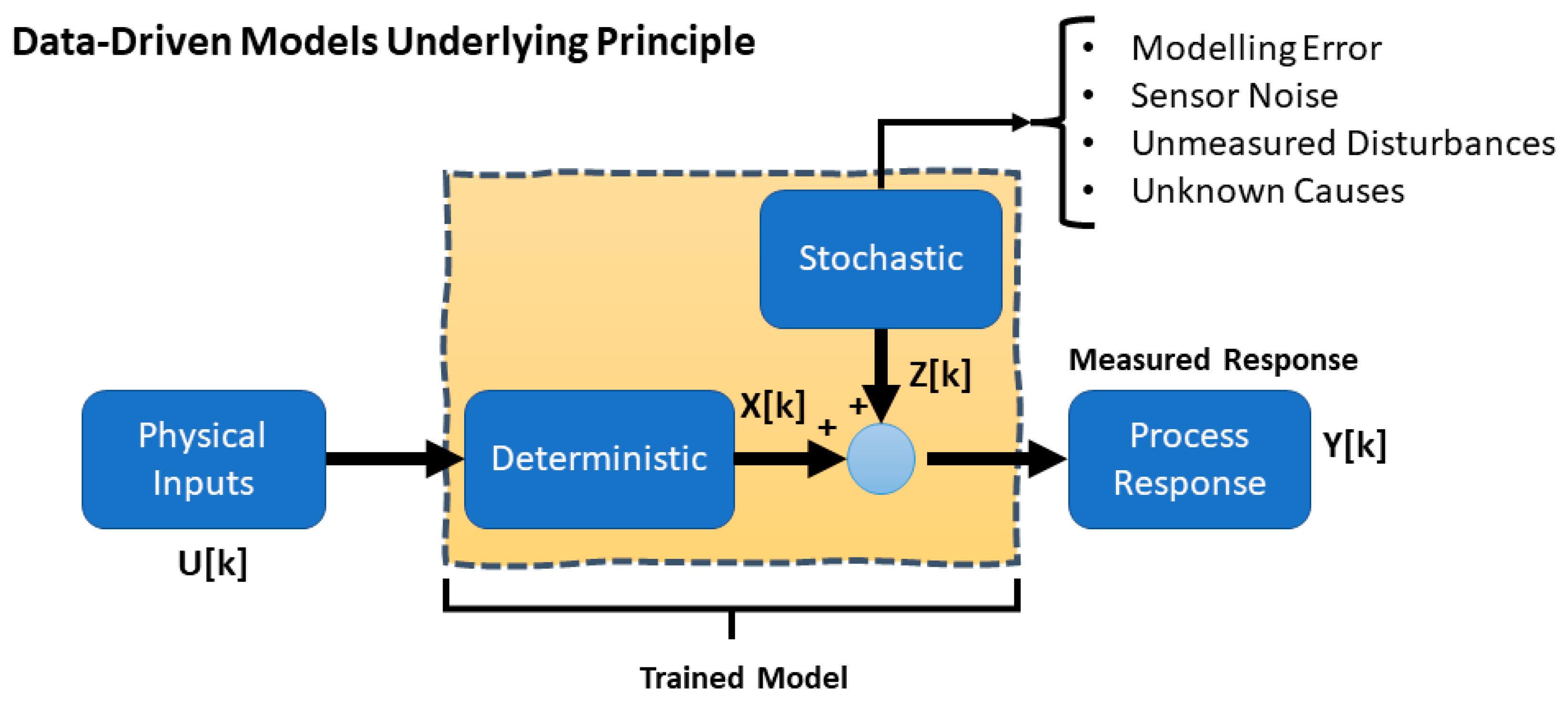
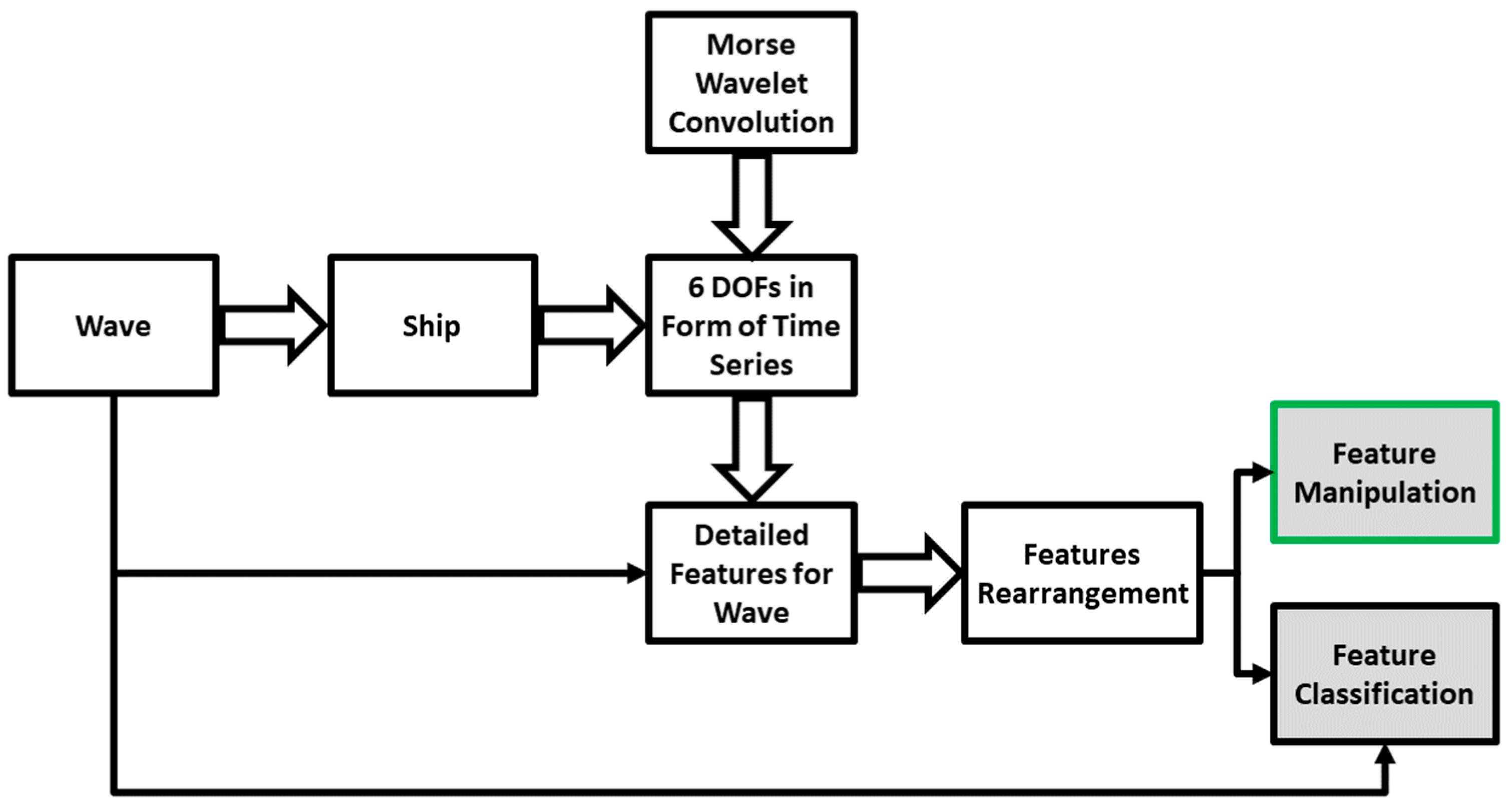
Starting from the left side of the diagram, wave as the input excites the ship as the system, resulting in six DOF responses in the form of time series, the system output. The purpose of applying wavelet on the short pieces of time series is to extract as much information as possible from time series data in the form of detailed features representation. Further, these features are reorganized through numerical operation to facilitate eventual manipulation and classification based on the categorical wave classes. The final grey blocks indicated the outcomes of feature reorganization that could facilitate feature manipulation, or, in other words, direct control over the densified features. Additionally, feature classification can lighten the training cost, which is aimed at being the focus of part B of the current issue.

The data generation process up to the output has been explained in Section 2. Nevertheless, six DOFS must be represented as a specific form for further mathematical operation. To include all features in the data, an additive approach has been adopted according to [15], representing every three DOFs of translational $\left(\mathrm{x},\mathrm{y},\mathrm{z}\right)$ and angular motions $\left(\varphi ,\mathsf{\theta },\mathsf{\psi }\right)$ to a condensed vector resulting from the summation of DOFs. The pertinent reason is simply due to the complex interaction of the mooring system’s impact on floating object responses and the mutual effects of responses. The vectors obtained from the summation of each three DOFs are normalized between (0,1) and represent a unique vector of $\mathsf{\varsigma }\left(\mathrm{k}\right)$ by summation of ${\mathrm{y}}_{\mathrm{d}}\left[\mathrm{k}\right]$ where $d=1,2$ denoting each group of normalized DOFs. The matrix given in Equation (3), indicating summation of the six DOFs. For a vector $\mathsf{\varsigma }\left(\mathrm{k}\right)$ representing the sphere/ship response, $\mathrm{k}$ denotes the discrete sample instant, and $l$ the length of the vector, taken in this study as 40 s, corresponding to 8000 samples. However, noting that for the first part of the study addressing the deterministic input–output, only heave response is considered.

$$\mathsf{\varsigma }{\left(\mathrm{k}\right)}_l={{\displaystyle \sum }}_{d=1}^6{y}_d{\left[\mathrm{k}\right]}_l$$

(3)

To capture detailed spectral-temporal features from sphere responses corresponding to various waves, we employed the Morse wavelet. This wavelet, formed by combining complex exponential and Gaussian windows, offers distinct advantages as outlined in [29]. Specifically, the generalized Morse wavelet is utilized with parameters, such as symmetry ($\gamma$), set to be 3, and time-bandwidth $p^2$ set to 60. This analytical wavelet, characterized by a scaling factor, acts as a filter bank, allowing to systematically extract detailed spectral-temporal features, convolving over the observation window. The benefits of representing these features via a scalogram, discussed extensively in [24], surpass alternative Fourier and wavelet-based methods. Equation (4) illustrates the wavelet function, where $\mathrm{U}\left(\mathsf{\omega }\right)$ represents the unit step, $a_{\beta ,\gamma }$ is a normalizing constant, and $\omega$ denotes frequency, with $m$ and $n$ determining the matrix arguments, resulting in $\Psi$ as a wavelet.

$${\Psi }_{p,\gamma }=\mathrm{U}\left(\mathsf{\omega }\right) a_{\beta ,\gamma } {\omega }^{{\displaystyle \frac{p^2}{\gamma }}}{e}^{-{\omega }^{\gamma }}$$

(4)

The 2D matrix of ${\mathsf{\Gamma }}_{\mathrm{m},\mathrm{n}} \left(\mathrm{k}\right)$ as the result of wavelet coefficients can be represented by an image, which helps for better visual perception of the spectral constitution of a signal and features amplitude over a fixed temporal direction (40 s). The image can be formed in the RGB channel; however, it has turned into grayscale with a normalized value between 0 and 1 for all pixels due to computational efficiency and less sensitivity to noise [24]. The corresponding 2D matrix, ${\mathsf{\Gamma }}_{\mathrm{m},\mathrm{n}} \left(\mathrm{k}\right)$ can be transformed into a [256 × 256] grayscale image using a linear conversion described in Equations (5) and (6). Here, the pixel value is determined by ${\rm Y}$, which serves as a scale factor adjusting the pixel intensity between 0 and 255, and $\xi$, the shift parameter, represents a constant that can be adjusted to control brightness, which is taken as 0 here.

$${\mathsf{\Gamma }}_{\mathrm{m},\mathrm{n}} \left(\mathrm{k}\right)={\Psi }_{p,\gamma }\times \mathsf{\varsigma }\left(\mathrm{k}\right)$$

(5)

$${\mathrm{P}}_{\mathrm{m},\mathrm{n}}={\rm Y} \times {\mathsf{\Gamma }}_{\mathrm{m},\mathrm{n}}\left(\mathrm{k}\right)+\xi$$

(6)

Therefore, through sliding Equation (6) to all $m$ and $n$ values of ${\mathsf{\Gamma }}_{\mathrm{m},\mathrm{n}} \left(\mathrm{k}\right)$ results in matrix ${\mathrm{P}}_{\mathrm{m},\mathrm{n}}$, where $\mathrm{P}$ represents the pixel intensity values ranging between 0 and 255, and m and n are both 256. 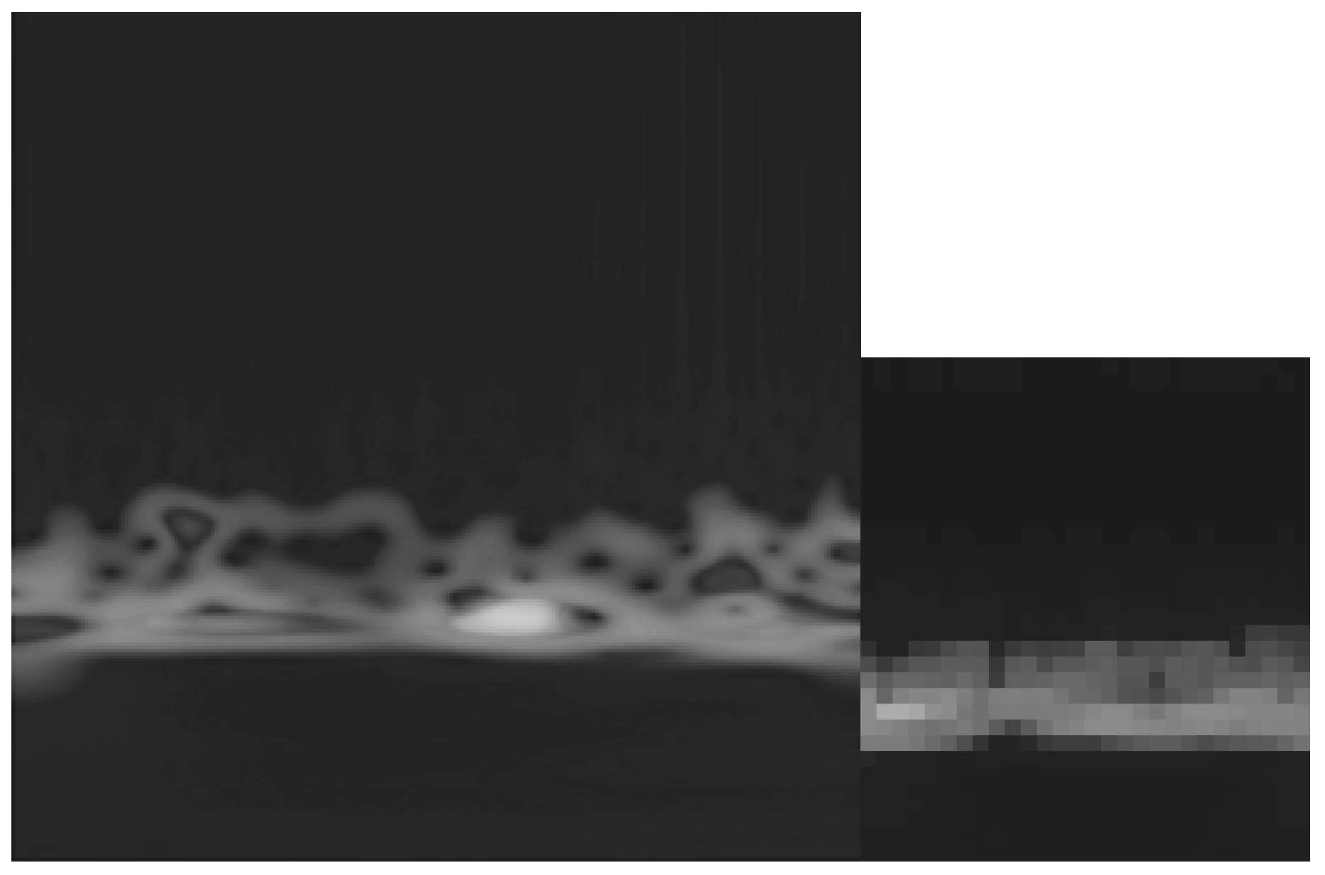Subsequently, the pixel values are normalized to a range between 0 and 1 using Equation (7), resulting in the vector ${\mathsf{{\rm K}}}_{\mathrm{a},\mathrm{b}}$, where $a$ equals 256 and $b$ equals 1, turning the matrix into a column vector. 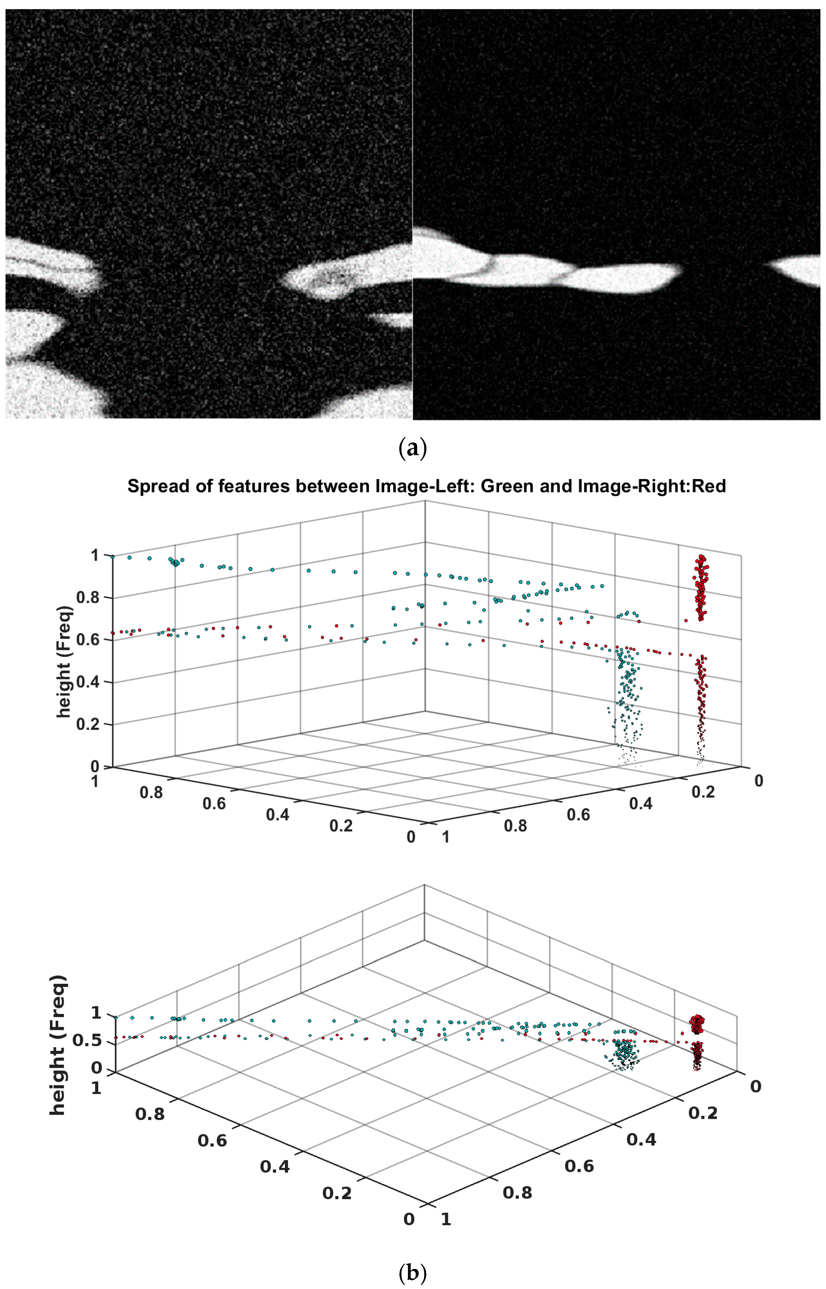To have a better visual representation, Figure 7a indicates the cumulative scalogram of $\mathsf{\varsigma }\left(\mathrm{k}\right)$ and subsequent transformation of vector $\mathsf{{\rm K}}$ on a diagonal plane within the new space in Figure 7b. This depicts the result of six DOFs accumulation for a single observation of 40 s. As can be witnessed, the features stand out differently for each image, corresponding to different time stamps of the sphere’s response to the wave.

$${\mathsf{{\rm K}}}_{\mathrm{a},\mathrm{b}}={\displaystyle \frac{{{\displaystyle \sum }}_{\mathrm{m}=1}^{256}P}{max{{\displaystyle \sum }}_{\mathrm{m}=1}^{256}P}}$$

(7)

In Figure 7a (left image), the scalogram is depicted in grayscale, overlaid with white Gaussian noise with a variance of ${\sigma }^2=0.01$, corresponding to a signal-to-noise ratio (SNR) of 8.99. This noise is visually represented as a scattered pattern of white pixels across the scalogram. As can be seen in Figure 7a, the noise manifested within new feature space in higher variation and feature spread for the range of pixel intensity below 0.5. Apart from that, the pixels shifted in the range below 0.5 due to the higher average value of the vector. Thus, the noise variance can be correlated with the features spread in new space qualitatively and quantitatively. Zooming in on the primary low-frequency components of Figure 7a, prominently visible as a broad white region in Figure 7a (left image) and (right image), reveals their consistent influence across the diagonal spread in Figure 7b above 0.5, akin to the significant features. Acknowledging the reverse spectral direction in the new feature space, noting that upper regions in image height direction attribute to lower frequency constitution, while lower regions represent higher frequencies. As such, the lower spectral elements, white pixels in the bottom of the left image in Figure 7a, show up at the higher height of Figure 7b.

By and large, the new operation compressed the features in the temporal direction while preserving the spectral constitution through normalized wavelet coefficients not only in the temporal direction but also given the intensity of pixels amplitude in the spectral direction. This densifies the nuanced information within the 40 s of the time series, shrunk into a vector as a single information packet, either for further classification or regression purposes. Data transformation in this way gives a new insight into features spread and constitution, where they can be worked out, i.e., reorganized, sorted, etc., and finally linked with the inputs. To elaborate further, while the direct noise observed in the accelerometer of the inertia measurement unit (IMU) exhibits a random walk behavior [30] and can be effectively filtered in the time series data collected from sensors, its influence on feature distribution remains uncertain. This influence becomes more pronounced, especially in the context of feature clustering concerning the classification of wave classes (labels), and the limitation of current work can be the scope of further studies.

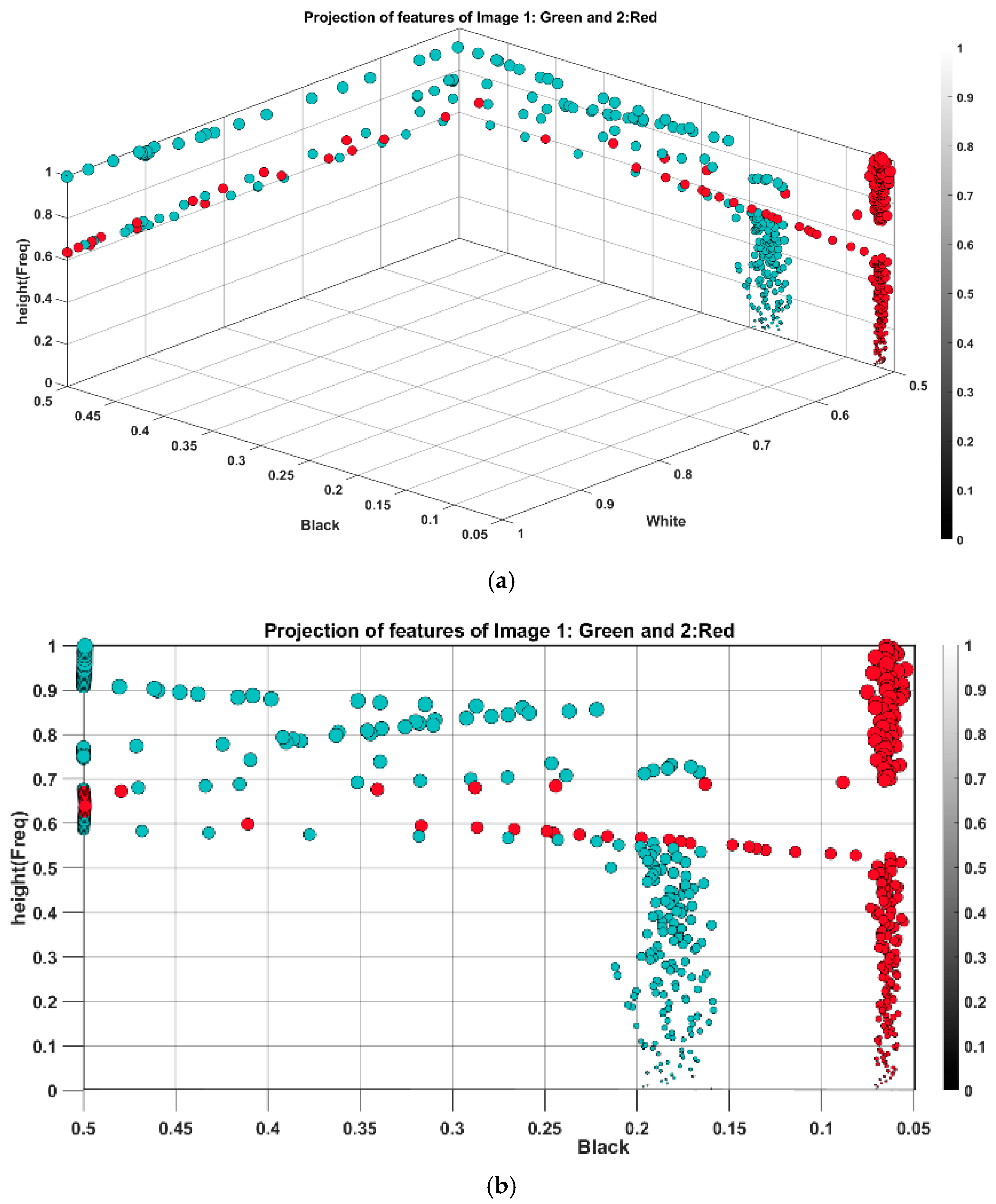
The transformation reorganizes new features, presenting different approaches with unique benefits and challenges. This will be explored in the next paper, part B, focusing on how feature reorganization impacts computational efficiency and classification. For the current analysis, features on the diagonal plane have been projected into two planes based on the pixel’s intensity stratification. Using Equations (5) and (6), higher amplitudes in the sequence of $y_d\left[k\right]$ correspond to higher pixel intensities, approaching white (or 1) in the scalogram. A threshold value of 0.5 splits the features for projection: those below 0.5 are projected onto the plane called “black”, while those above are projected onto the “white” plane. This sieving not only provides insight into the spectral elements but also their contribution within the vector. More accurately, vector $\mathrm{k}$ is reconstructed in two vectors of the same size $\mathrm{A}, \mathrm{B}$, where the vectors ${\mathrm{A}}_{\mathrm{a},\mathrm{b}}$ and ${\mathrm{B}}_{\mathrm{a},\mathrm{b}}$ are composed of dummy values of 0.5 in arguments and $\mathrm{K}\le 0.5$ for $\mathrm{A}$ and $\mathrm{K}>0.5$ for $\mathrm{B}$. Figure 8 shows the projection of features into black and white planes with the color bar representing pixel intensity.

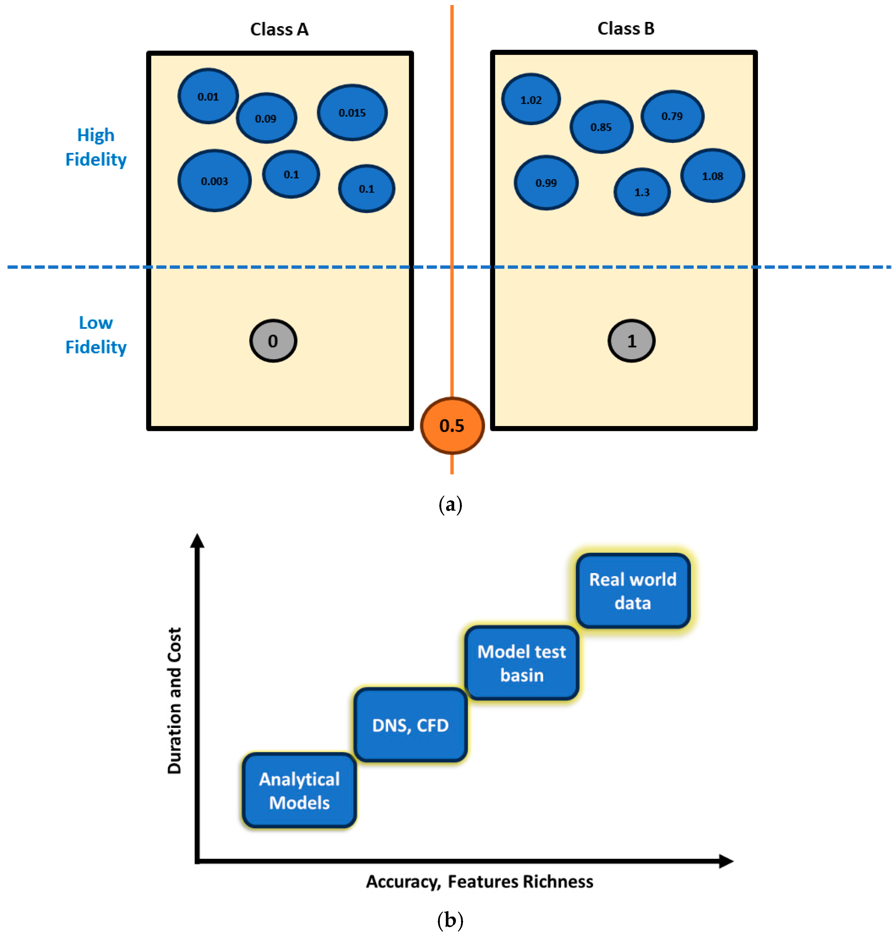
Engineered data possess twofold advantages: Firstly, this facilitates monitoring features spread not only from different exciting forces but also different data generation processes. For example, it shows how the features from the model test and synthesized data differ in distribution, and this insight can be further utilized for feature transformation between different fidelity level modeling that is the focal point of the present study. Secondly, engineered features can be reorganized as new unique attributes, ranging between 0 and 1, which can positively enhance classification and reduce training costs, as the second outcome of feature engineering in Figure 6, which will be discussed in part B of the current issue.

3.2. Evaluation for Deterministic Inputs (Regular Waves)

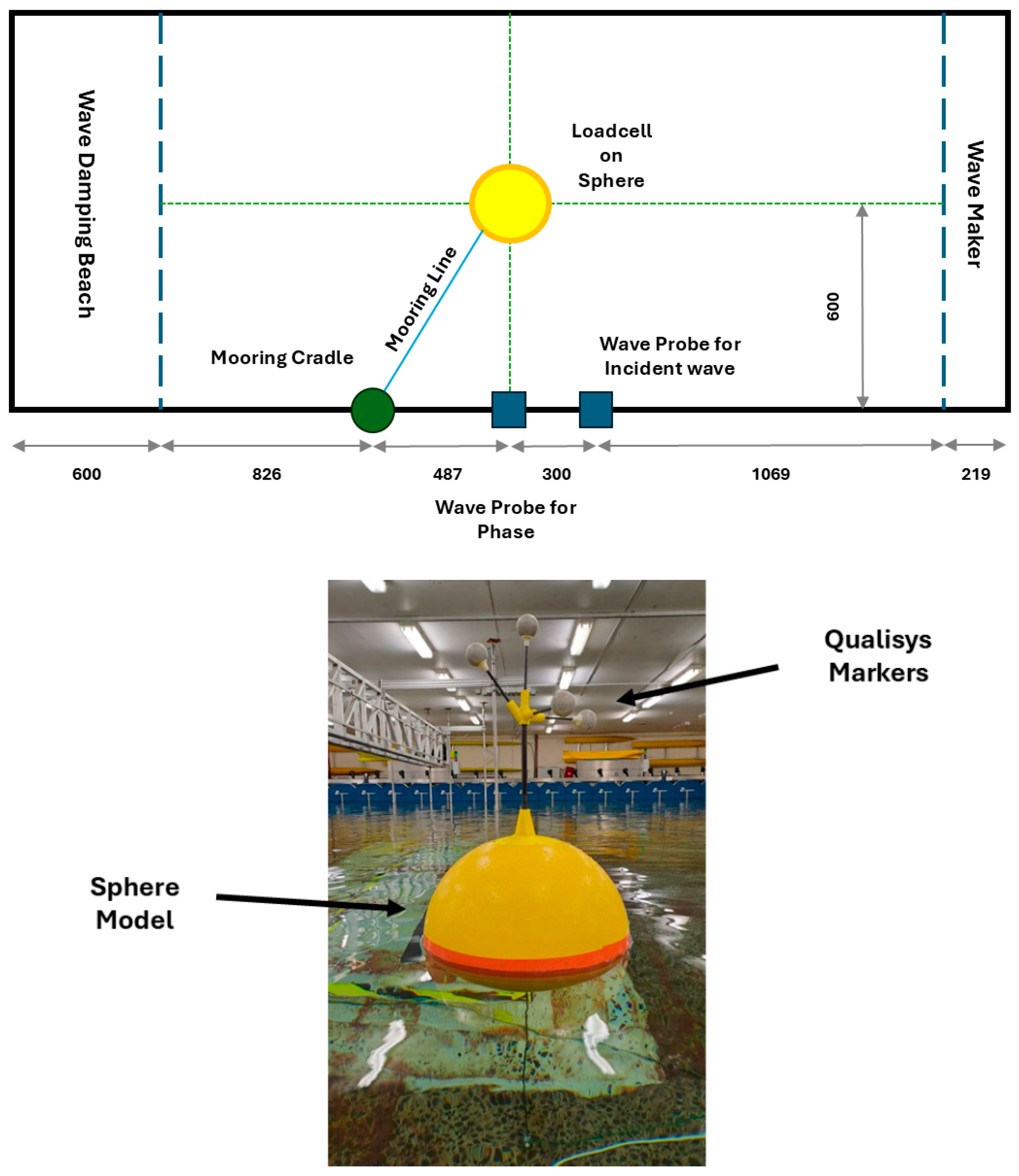
Although wave elevation patterns possess random characteristics, they can be broken down to the superposition of many numbers of deterministic sinusoidal waves [31,32]. Unlike free response, which reflects the system characteristics (sphere), the deterministic input determines the forced response of the system excited by inputs [9]. As mentioned, the new space projection enables monitoring and investigating features produced by different data generation processes. To examine this, the test ran first with a deterministic input–output relationship known as regular waves based on one DOF, heave ($z$). It basically contains an exciting sphere in the wave basin; further, the simulation in ANSYS AQWA using a sinusoidal wave and (response amplitude operator) RAO-based response. The test was carried out on the heave response in a range of wave periods, starting with close periods of 1.1 and 1.0 s. 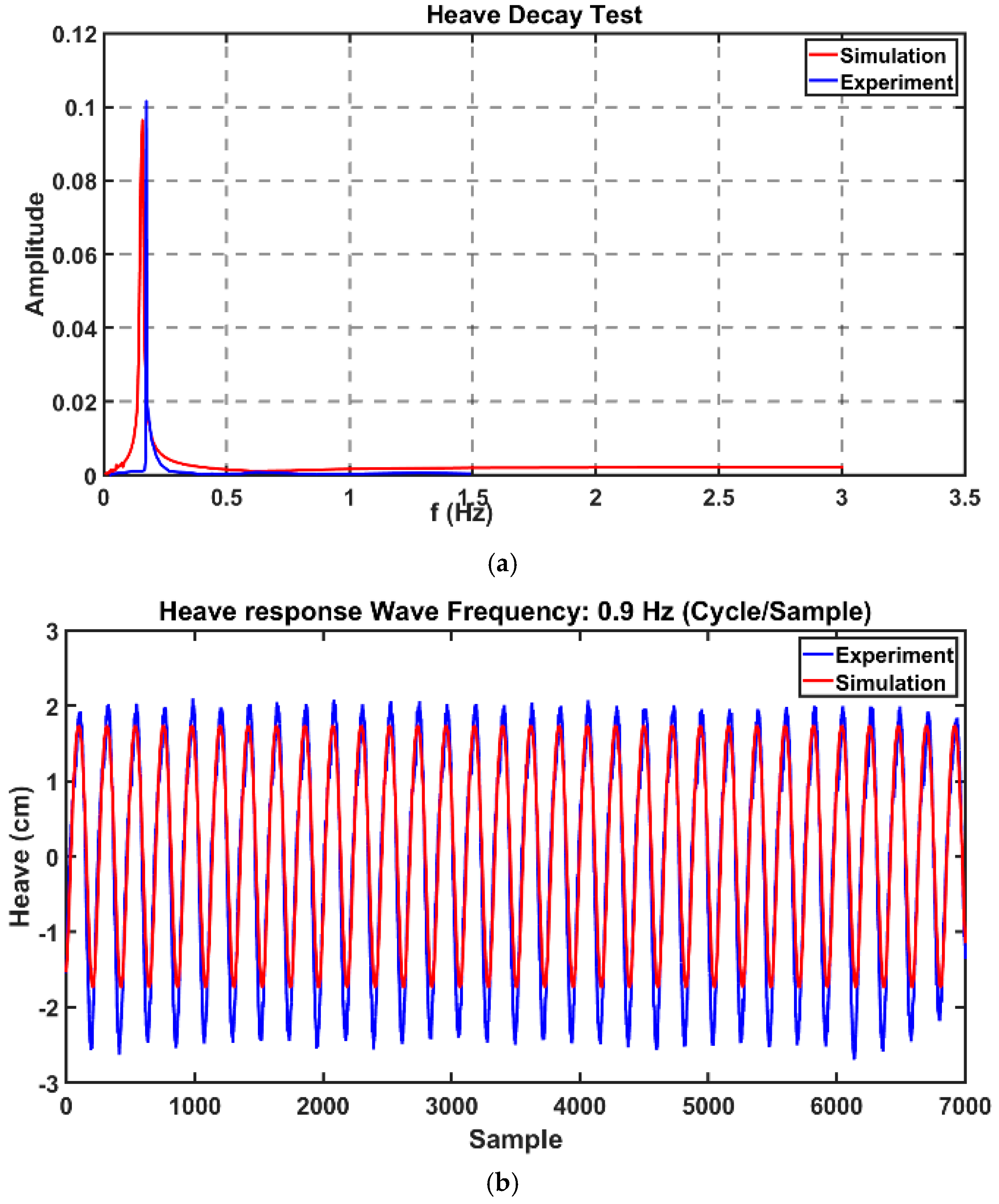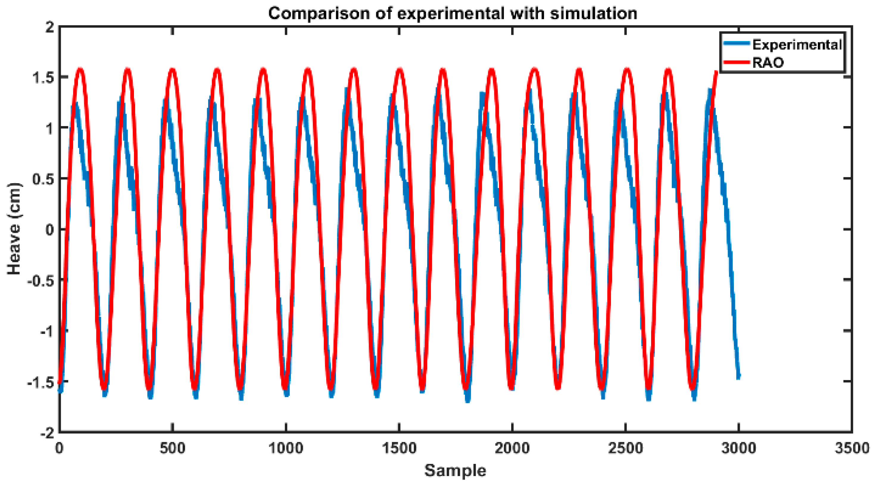Figure 9 pictures the comparison of experimental and simulation results for sphere heave response for the respective waves. As can be observed, the simulation well met the experimental results apart from minor discrepancies. 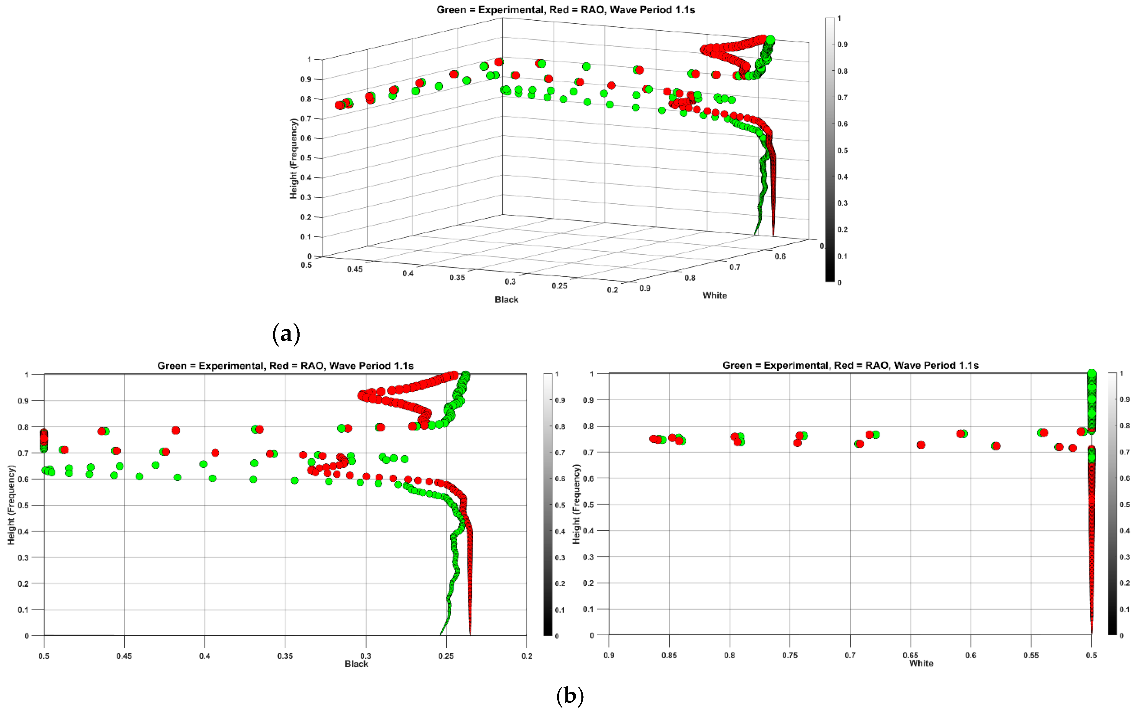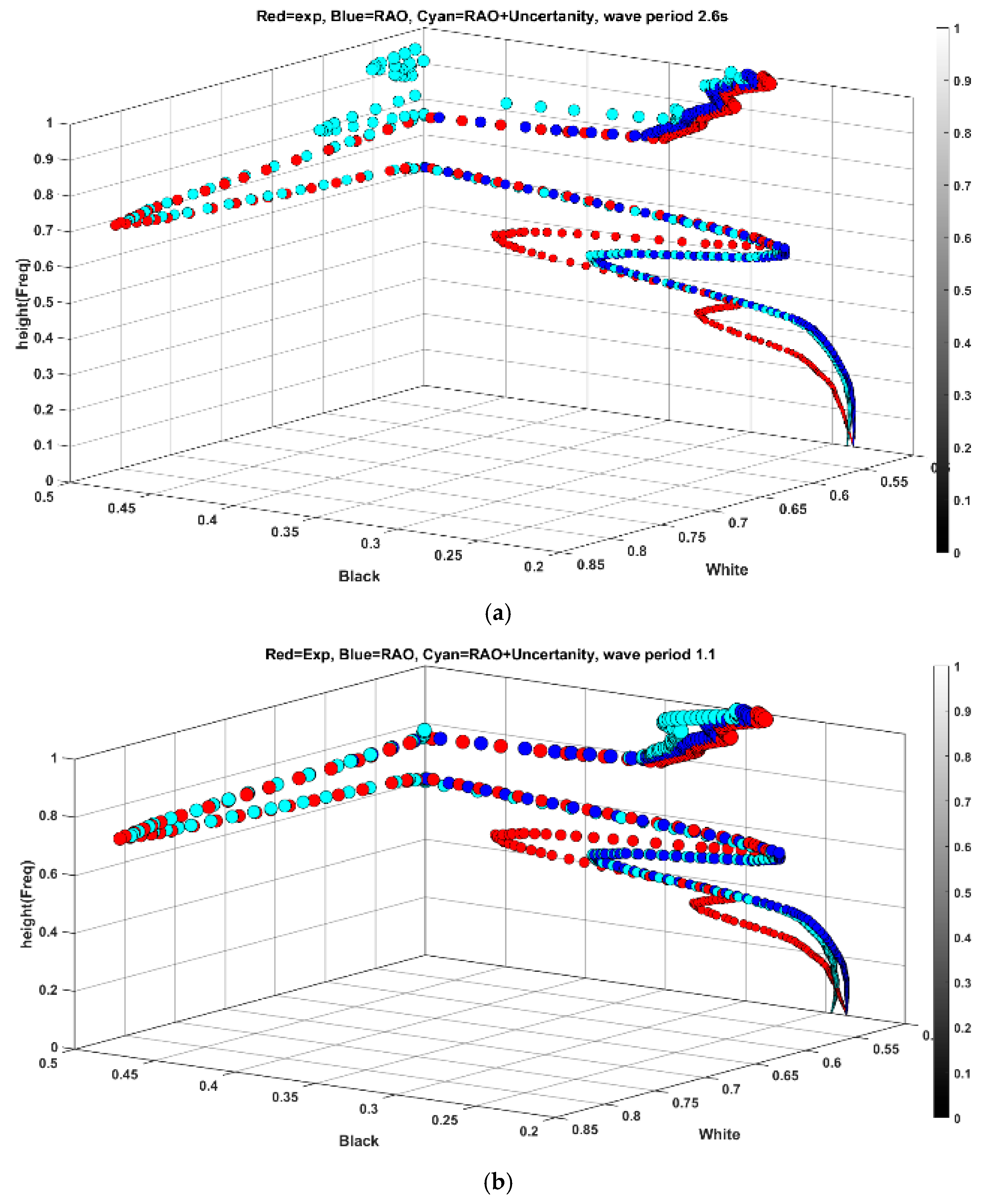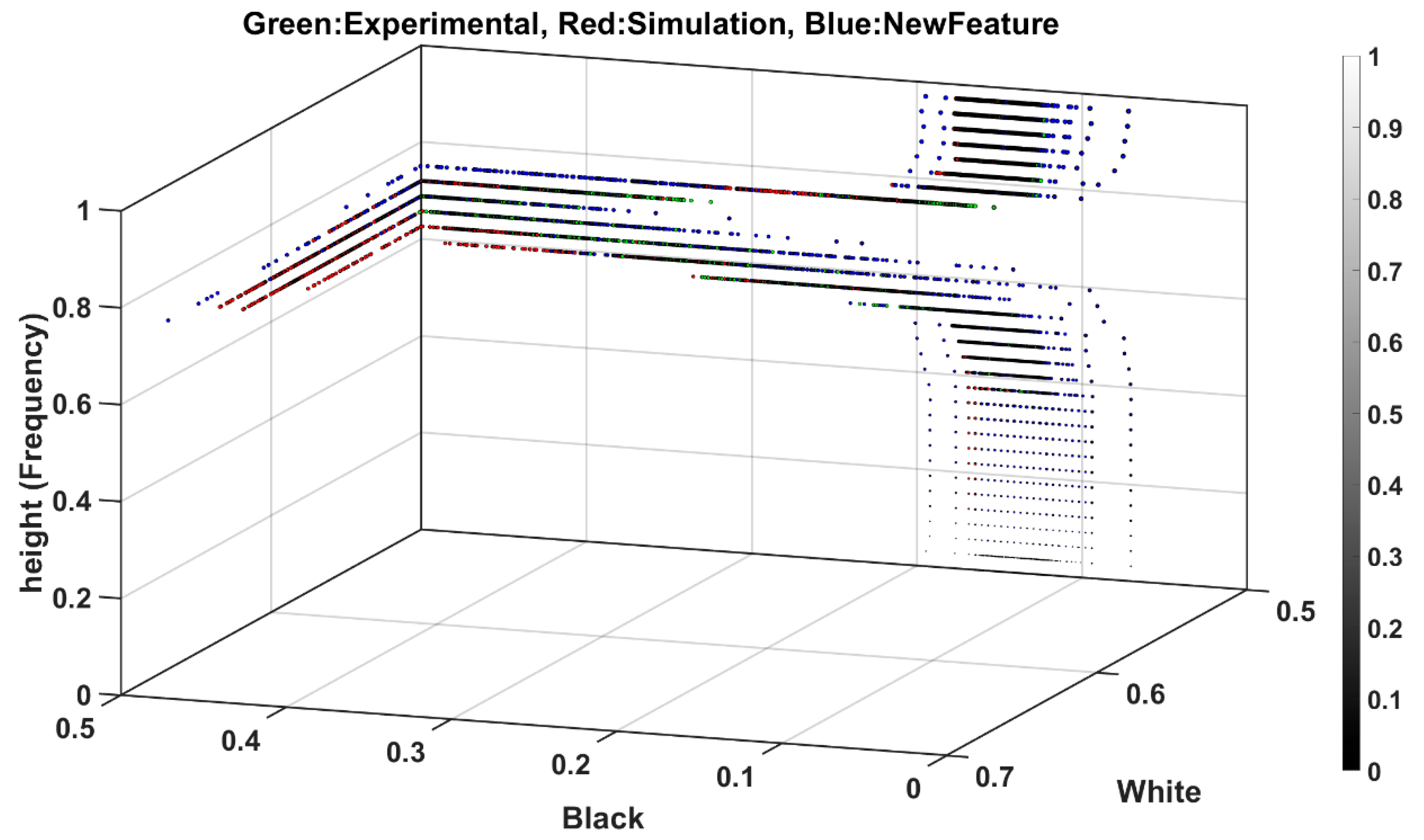Figure 10 indicates the results of feature spread projection for a heave period of 1.1 s. Figure 10a indicates the projection of features from experimental tests and simulations in 3D space, and Figure 10b shows the projection of vectors in white and black planes. According to Figure 10b, the difference between features accumulated more in high-frequency regions with less signal amplitude (blackish pixels), whereas the difference in low-frequency regions with higher amplitude is less pronounced with quite a similar pattern.

Examining the planes in Figure 10b, it is evident that the low-frequency traits, depicted in the white plane, remain consistent and nearly identical between experiment and simulation. However, notable disparities emerge in the projection onto the black plane, despite overall spread similarities. As noted earlier, the presence of noise amplifies the variance in feature distribution, a trend also observed in black plane values below 0.5, mirroring the behavior seen in Figure 7. This discrepancy can be attributed to inherent uncertainties in the experiment, which are challenging to replicate in numerical simulations.

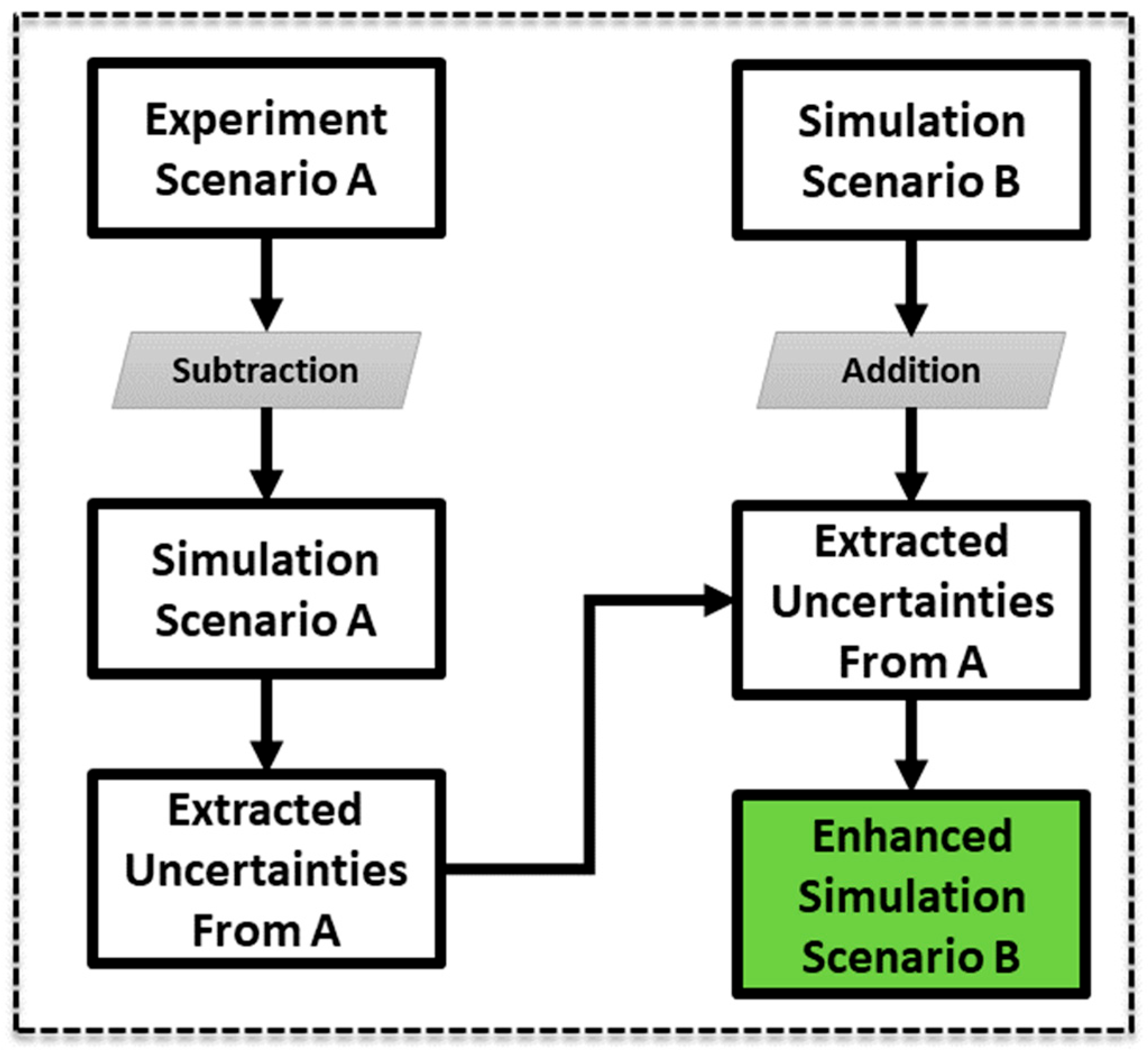
Revisiting primary objectives, integrating entropy is vital for ML applications, as demonstrated in Figure 11, showcasing the proposed method for enhancing simulation outcomes through uncertainty integration. In essence, the features of simulation data with a period of 1.1 s are subtracted from the experimental data in each plane, and the residual features are combined with those obtained from simulation with (another period) a period of 1.0 s. To this end, the vector ${\mathsf{{\rm K}}}_{\mathrm{a},\mathrm{b}}$ as the sphere response from the experiment, which includes only ${\mathrm{y}}_{\mathrm{z}}\left[\mathrm{k}\right]$ for heave, is reconstructed in two vectors of ${\mathrm{w}}_{\mathrm{a},\mathrm{b}}$ and ${\mathrm{q}}_{\mathrm{a},\mathrm{b}}$, where $a=1$ and $b=256$, and they are projected on white and black planes, respectively. The same operation has been carried out for vector ${\mathrm{K}}_{\mathrm{a},\mathrm{b}}^{\prime }$ as the result of simulation as well as projection vectors ${\mathrm{w}}_{\mathrm{a},\mathrm{b}}^{\prime }$ and ${\mathrm{q}}_{\mathrm{a},\mathrm{b}}^{\prime }$. Equation (8) shows the simple algebraic subtraction that yields the residual features $W_{a,b}$ and $Q_{a,b}$.

$${\mathrm{W}}_{\mathrm{a},\mathrm{b}}={ \mathrm{w}}_{\mathrm{a},\mathrm{b}}-{\mathrm{w}}_{\mathrm{a},\mathrm{b}}^{\prime }, {\mathrm{Q}}_{\mathrm{a},\mathrm{b}}={ \mathrm{q}}_{\mathrm{a},\mathrm{b}}-{\mathrm{q}}_{\mathrm{a},\mathrm{b}}^{\prime }$$

(8)

Considering the same operation for scenario B with ${\mathrm{V}}_{\mathrm{a},\mathrm{b}}$, the vector of response simulation for period 1.0 s and ${\mathrm{t}}_{\mathrm{a},\mathrm{b}}$ and ${\mathrm{l}}_{\mathrm{a},\mathrm{b}}$, the projection vectors, the new vectors that will be compared with scenario B (experimental data) can be obtained from Equation (9). ${\mathrm{T}}_{\mathrm{a},\mathrm{b}}$ denotes the enhanced features on white planes and ${\mathrm{L}}_{\mathrm{a},\mathrm{b}}$ on black planes.

$${\mathrm{T}}_{\mathrm{a},\mathrm{b}}={\mathrm{W}}_{\mathrm{a},\mathrm{b}}+{ \mathrm{t}}_{\mathrm{a},\mathrm{b}}, {\mathrm{L}}_{\mathrm{a},\mathrm{b}}={ \mathrm{Q}}_{\mathrm{a},\mathrm{b}}+{ \mathrm{l}}_{\mathrm{a},\mathrm{b}}$$

(9)

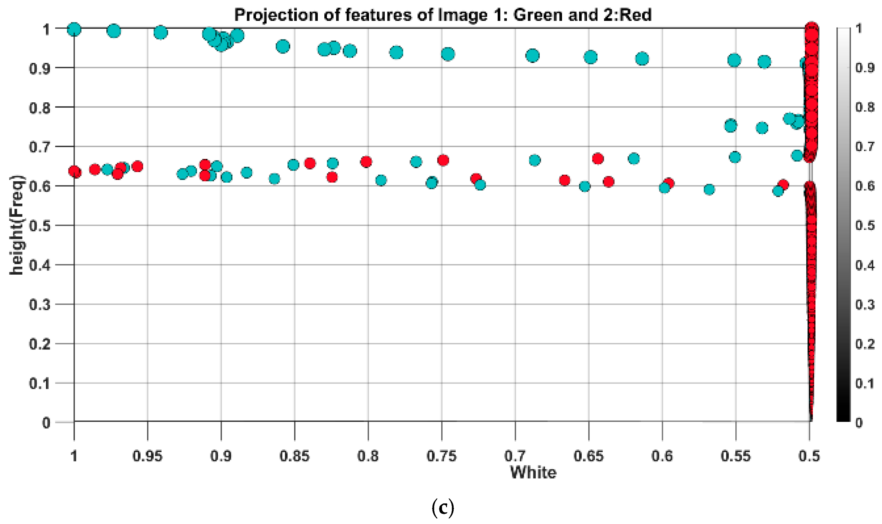
As it had been surmised, the new feature spread in the resulted vectors must show a closer distribution to the experimental data of new period 1.0 s in comparison with the simulation. Figure 12 indicates the features spread for vectors on the black plane for wave period 1.0, scenario B. As can be seen visually, the cyan color data represent the new spread that is qualitatively closer to experimental data. Regardless, the result must be evaluated quantitatively, so the root mean square error (RMSE) value between features has been adopted to quantify the overall magnitude of error. In the black projection plane, the RMSE between new features and experimental data was found to be 0.0738, whereas the RMSE between RAO-based simulation and experimental data is 0.0872. However, cyan and blue points matched for the white plane, and the RMSE for both is 0.792. To conclude, the proposed feature space framework has improved the simulation data in a higher frequency range, even though further investigation is necessary to check the functionality of a broader spectral range.

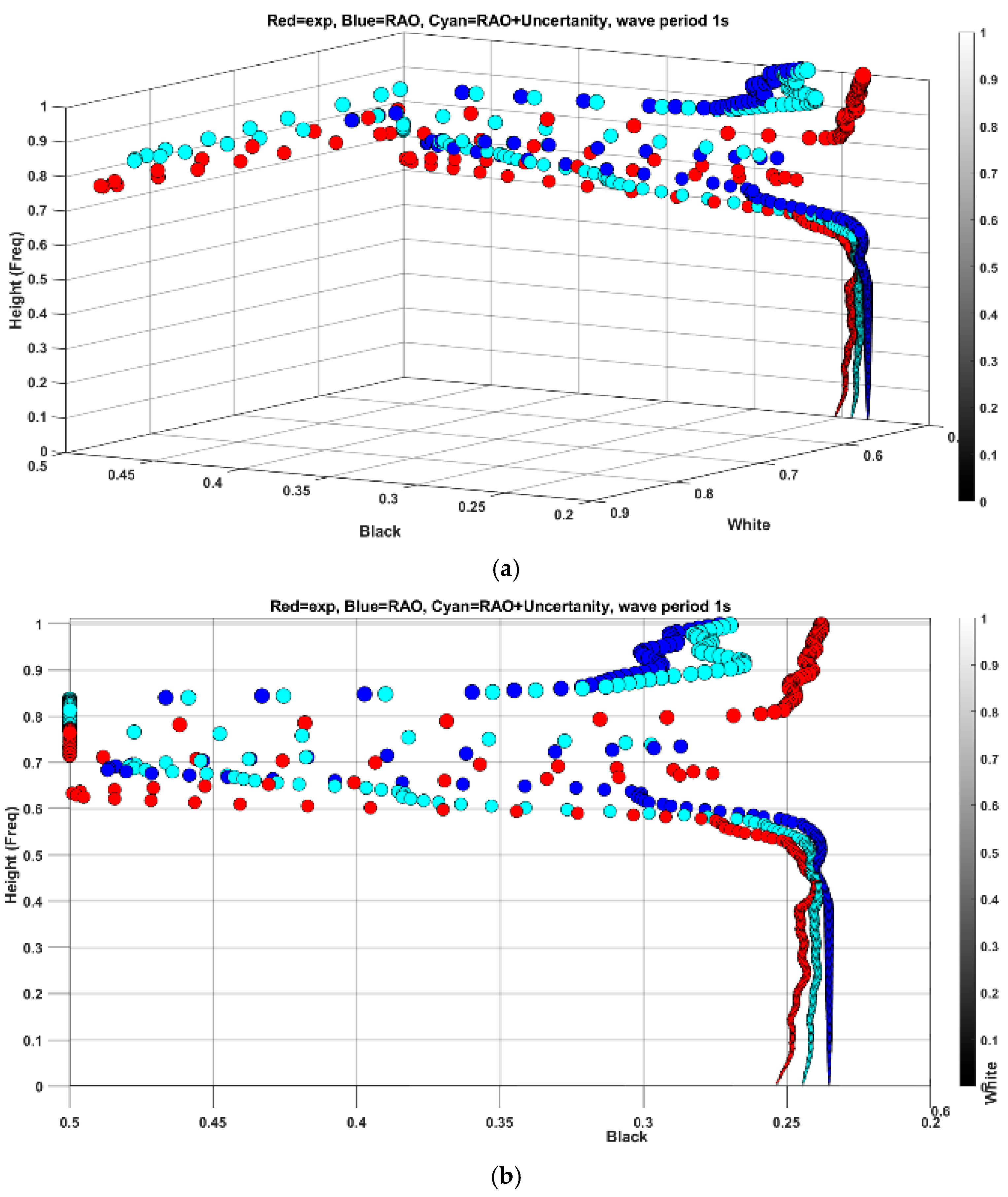
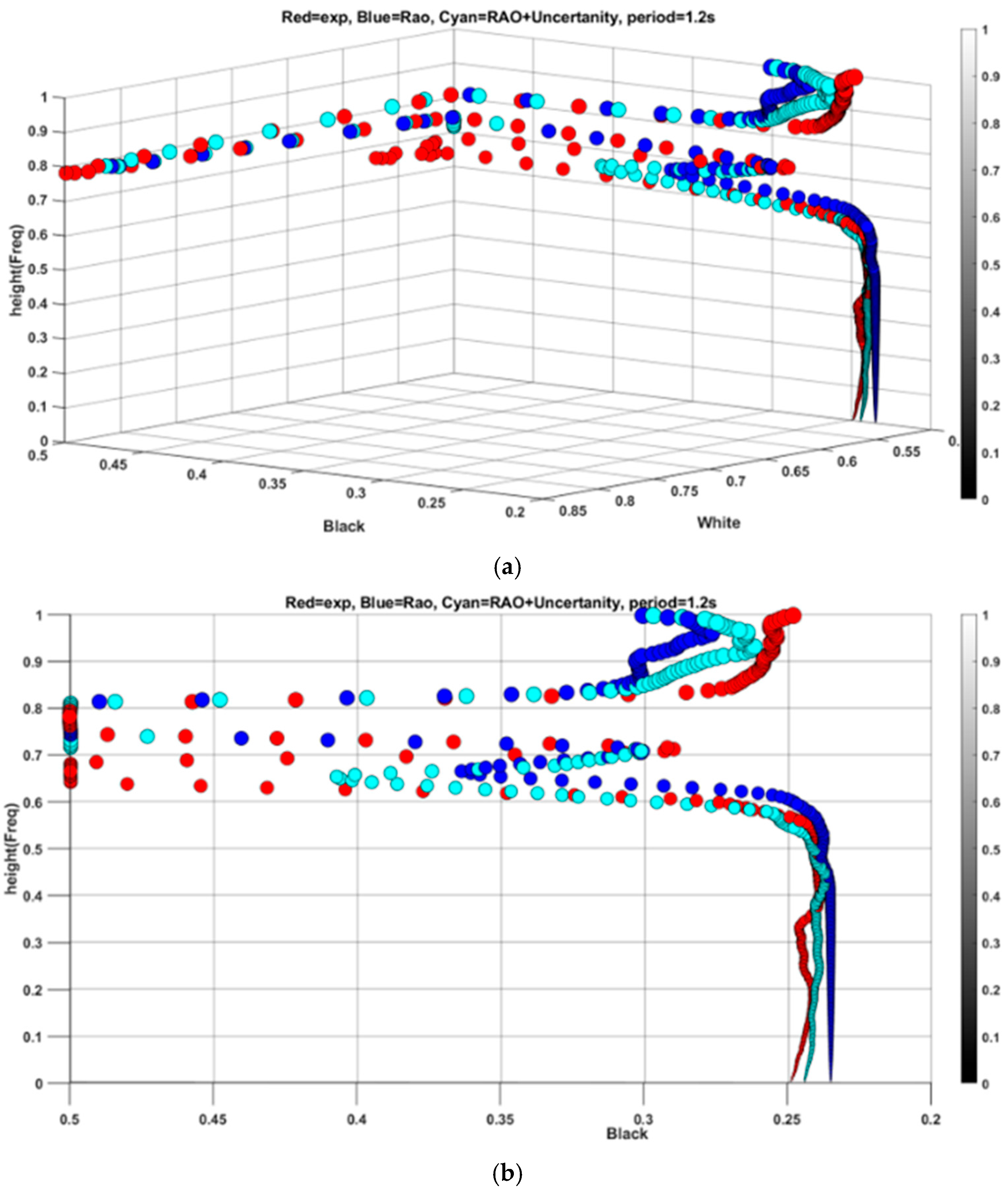
While the proposed method has shown effectiveness for frequencies in a narrow range, it is essential to explore a broader spectrum. To achieve this, periods of 1.2 s, 2.6 s, 2.8 s, and 1.8 s have been selected for analysis. Beginning with a period of 1.2 s, which is close to the base period of 1.1 s, the residual features are combined with simulation data based on RAO with a period of 1.2 s as indicated in Figure 13. Figure 14a displays the time series of the heave responses for both experimental and simulated data. In Figure 13, the RMSE values for the black plane are determined to be 0.0415 for the new feature and 0.0450 for the RAO-based simulation. Meanwhile, the RMSE difference for the white plane is negligible, both at 0.0099. Upon observing the spread in both Figure 12 and Figure 13, it becomes apparent that the enhancement in features is predominantly concentrated in the lower height range below 0.5 on the color bar. By calculating the RMSE within this range, the new feature exhibits a significant decrease from 0.0084 to 0.0034. This improvement is attributed to the scaling property of the wavelet, which offers fine temporal resolution for high-frequency ranges and superior spectral resolution for low-frequency ranges.

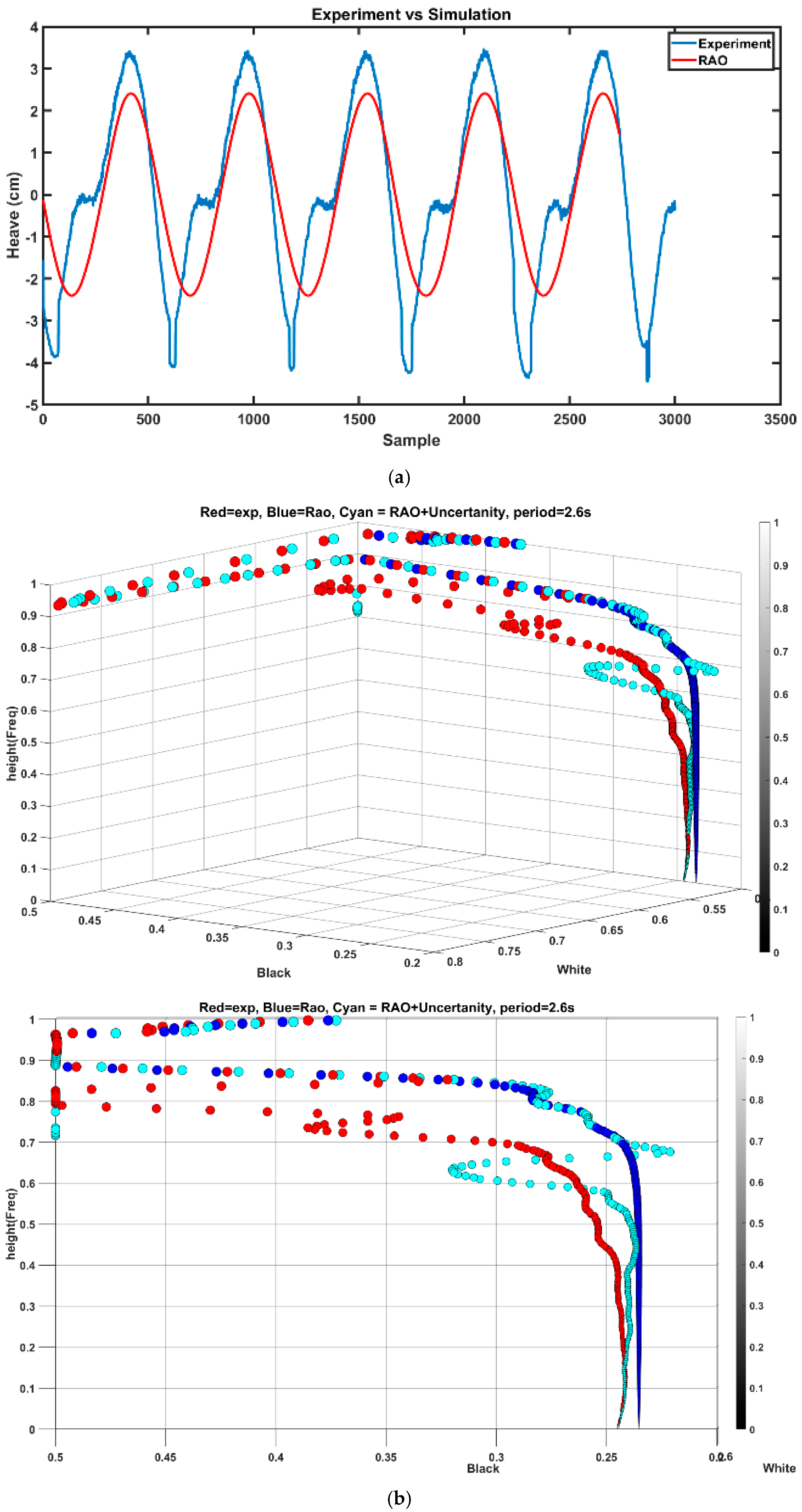
The deducted features obtained from period 1.1 s (${\mathrm{t}}_{\mathrm{a},\mathrm{b}},{\mathrm{l}}_{\mathrm{a},\mathrm{b}})$ has been utilized to low-frequency wave with a period of 2.8 s. Figure 14a illustrates the time series of heave response for both experiment and simulation (simulation is subscripted RAO), while Figure 14b displays the feature distribution. In this scenario, the RMSE value for the white plane is as expected, but it is lower for RAO-based simulation. However, for the high-frequency range of wavelet coefficients, less than 0.5 on the color bar, the RMSE for the new feature is 0.0062 compared to 0.0096 for the simulation. This indicates that the uncertainty in the test, regardless of the exciting force, remains relatively identical, which could be utilized for a specific range between different frequencies. This characteristic arises from the wavelet’s ability to extract nuanced temporal features in the high-frequency components of the data.

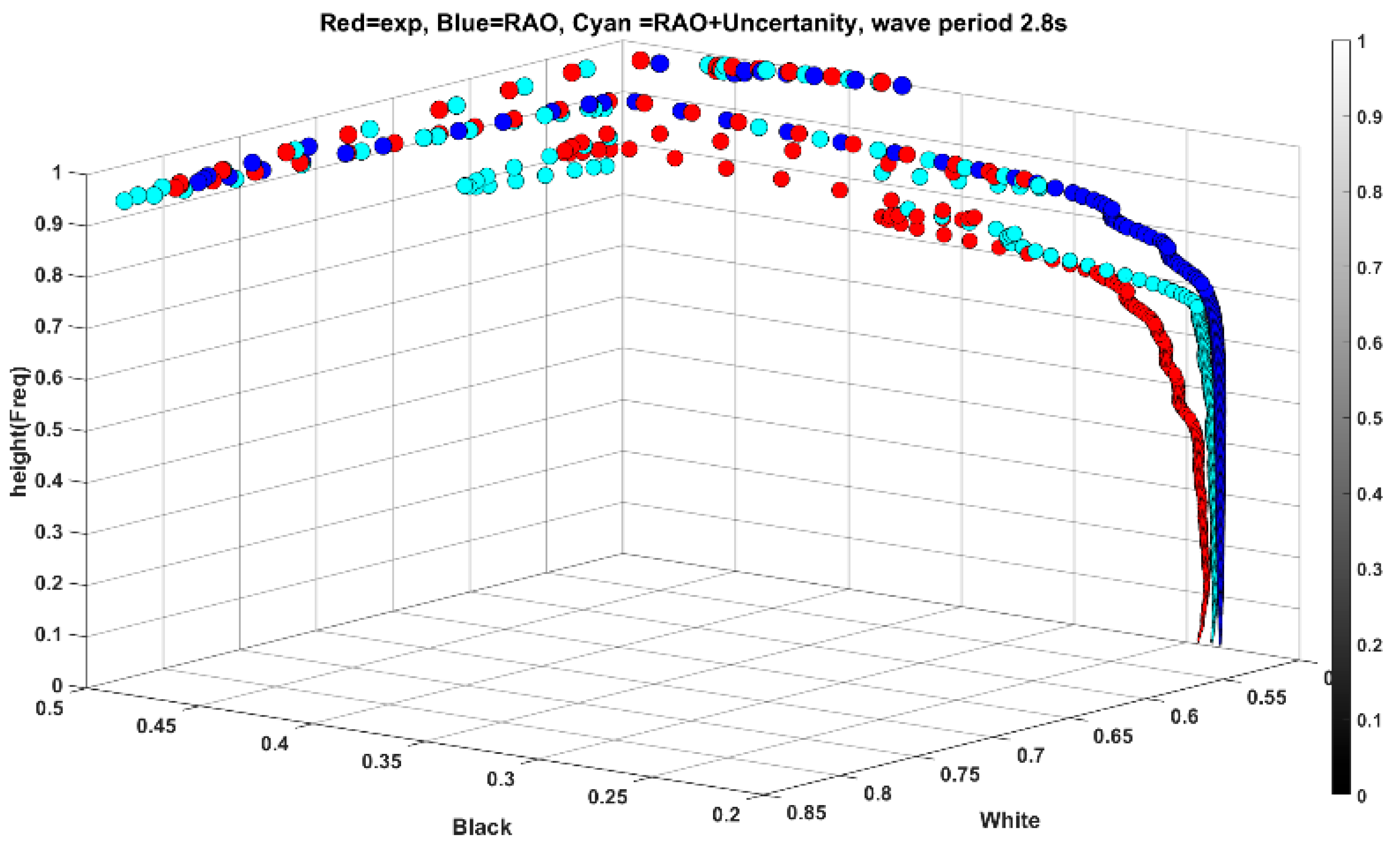
To further analyze the behavior of features within a close spectral range, the obtained features from a period of 2.6 s (as new scenario A) were utilized for simulations with a period of 2.8 s (as scenario B). This involved subtracting the features obtained from the experiment for the heave response of 2.6 s from the simulation features and adding the residuals $\left({\mathrm{t}}_{\mathrm{a},\mathrm{b}},{\mathrm{l}}_{\mathrm{a},\mathrm{b}}\right)$ to the simulation features of a period of 2.8 s $\left({\mathrm{T}}_{\mathrm{a},\mathrm{b}},{\mathrm{L}}_{\mathrm{a},\mathrm{b}}\right)$. As per Figure 15, the features’ spread shows a significant improvement compared to Figure 14b. Quantitatively, the RMSE for the black plane is 0.0611 for simulation and 0.0287 for the new features. In conclusion, it can be inferred that the technique performs effectively within a narrow frequency range and is functional for high-frequency components of distant frequencies.

At this juncture, the features obtained from high and low frequencies are compared with a frequency range close to the natural frequency of the heave response in the sphere, which is found to be a period of 1.8 s. Thus, the features obtained from a period of 2.6 s are tested. Figure 16a displays the results of applying the residuals from the period of 2.6 s to 1.8 s. Visually, it is apparent that apart from regions below 0.5 in the color bar, the rest of the data spread deviates from the experiment. However, the RMSE for the region below 0.5 has improved by 0.0493 and 0.0404 for simulation and new features, even though the overall RMSE is 0.0479 and 0.0598 for simulation and new features, respectively. To further explore this observation, another higher frequency wave with a period of 1.1 s is utilized. As depicted in Figure 16b, despite improvements in spread, the new feature slightly deviates in the low-frequency region with a higher intensity of black pixels. For the region below 0.5, the RMSE of the new feature is 0.0404 versus 0.0447 for simulation. 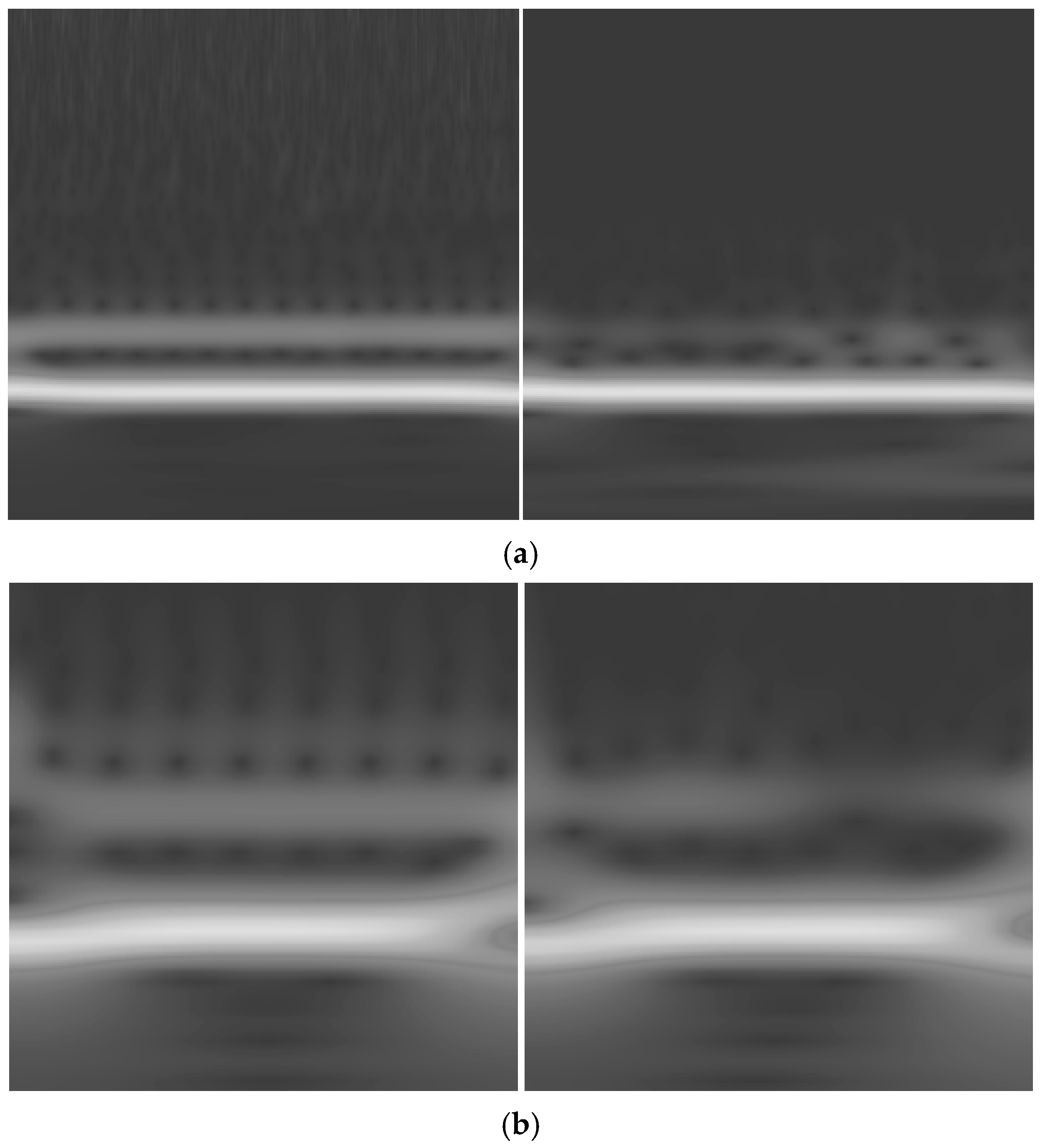These findings necessitate a more direct examination of the wavelet coefficients in the form of black and white pixel scalogram images as presented in Figure 17.

Based on Figure 17a, the upper half of the image displays arbitrary spectral components represented as jagged white lines, which are absent in the corresponding simulated data image with a period of 1.1 s. Similarly, this is also evident in Figure 17b for a period of 1.8 s. Upon closer inspection of the lower half, the experimental and simulation data appear nearly identical in low-frequency contribution. It was anticipated that close frequencies would exhibit similar shapes in the lower region, given that the RMSE values remained consistent.

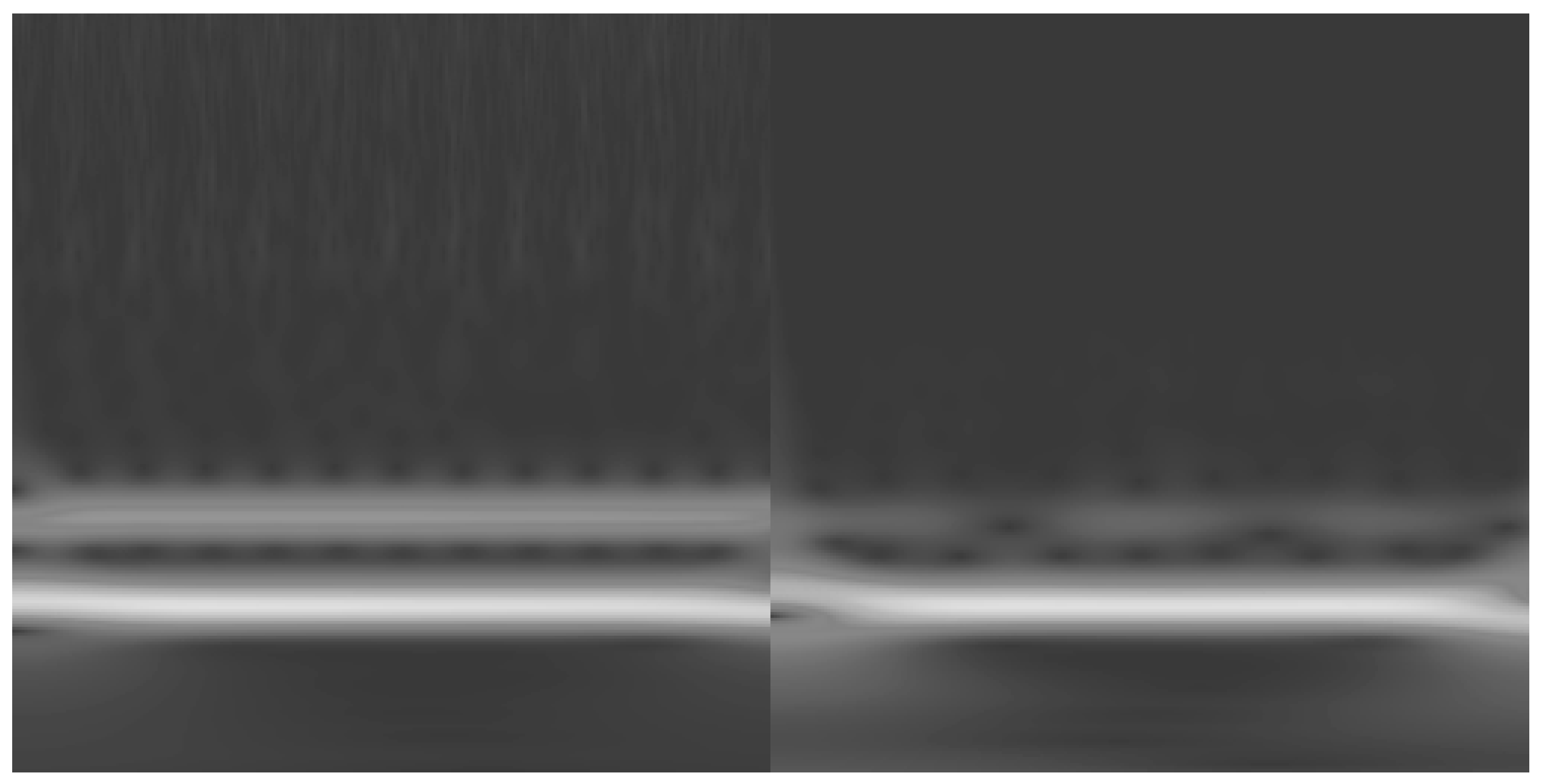
To this end, Figure 18 presents images of experimental and simulation data for a period of 1.2 s. Notably, aside from the upper half, both exhibit remarkable similarity. Moreover, the images from periods 1.1 s (Figure 17a) and 1.2 s appear similar in the lower half as well. These observations underscore the efficiency of the new feature spread mechanism for close frequency ranges. For instance, using one scenario in a test can replicate several close frequencies with minimal computational costs. However, when dealing with distant frequencies, the high spectral content can be effectively extracted from one experimental scenario and added to the simulation data. Consequently, the new approach can significantly enhance the accuracy, diversity, and entropy of simulation data for more real-world cases with minimal computational resources, achievable within seconds. This provides a better framework for designing experimental tests that can be directly or indirectly applied to generate more realistic and representative data for ML models.

4. Data Analysis Framework Application

After examining the proposed concept with deterministic data, this section delves into evaluating the framework for stochastic inputs. Additionally, discussions are provided for potential future use cases.

4.1. Irregular Waves Data

So far, the approach has utilized deterministic inputs for improved control and monitoring. However, field wave data are stochastic, demanding evaluation of the approach with stochastic wave inputs. To achieve this, the sphere model underwent testing in the model test basin (MTB). During this experiment, three instruments were utilized for data collection: resistive wave probes, a FUTEK QLA150 100 lb load cell, and a Qualisys motion capture system, which measured the free surface elevations, mooring loads, and motions of the sphere, respectively. The test was conducted to capture a broad range of spectral data sampled from the JONSWAP spectrum. The details of the test are reported in

Table 3. Detailed parameters of JONSWAP spectrum and wave parameters.

Wave Test Parameters
Scenario	Significant Wave Height (m), ${\mathit{H}}_{\mathit{s}}$	Peak Period, ${\mathit{T}}_{\mathit{p}}$	Run Time (s)	$\mathsf{\gamma }$	σ1	σ2	α
1	0.05	1.4	2400	1	0.07	0.09	0.0081
2	0.05	1.6	2400	1	0.07	0.09	0.0081
3	0.05	1.8	2400	1	0.07	0.09	0.0081

, and the parametric spectrum formulation for JONSWAP, $\mathrm{S}\left(\mathsf{\omega }\right),$ is given in Equation (10), where α denotes spectral energy parameter, $\left({\sigma }_1,{\sigma }_2\right)$ are spectral width parameters, $\gamma$ is peak enhancement factor, and $g$ is the gravity acceleration. The wave parameters, such as significant wave height $H_s$ and peak period $T_p$ in Equations (11), later can be derived from statistical moment $m_n$, applied on $\mathrm{S}\left(\mathsf{\omega }\right)$ by Equation (12).

$$\mathrm{S}\left(\mathsf{\omega }\right)={\displaystyle \frac{\alpha g^2}{16{\pi }^4}}{\omega }^{-5}exp\left[-{\displaystyle \frac{5}{4}}{\left({\displaystyle \frac{\omega }{{\omega }_p}}\right)}^{-4}\right]{\gamma }^b$$

(10)

$$b=exp\left[-{\displaystyle \frac{1}{2{\sigma }^2}}{\left({\displaystyle \frac{\omega }{{\omega }_m}}-1\right)}^2\right],\sigma =\left\{\begin{array}{c}{\sigma }_1 for \omega \le {\omega }_p\\ {\sigma }_2 for \omega >{\omega }_p \end{array}\right\}$$

$$H_s=4\sqrt{m_0}, T_p=2 \pi \sqrt{{\displaystyle \frac{m_0}{m_2}}}$$

(11)

$$m_n={{\displaystyle \int }}_0^{\infty }{\omega }^{n}S\left(\omega \right) d\omega$$

(12)

For regular waves, a single response was assessed, while for irregular waves, the final convolution vector was obtained by linearly adding four DOFs. This process involves surge and sway as translational motions forming vector $\mathsf{\xi }$, and roll and yaw as singular responses shaping vector $\mathsf{\psi }$. The method of vector addition and scalogram combination follows [24]. Four DOFs were used for consistency with ongoing research on advancing ships, using state-of-the-art simulator data from the MARITIME SIMULATION CENTRE of AMC.

The size of the data segment corresponding to a window size vector was fixed at 40 s. Additionally, to further investigate the effect of resolution, a max-pooling filter was applied. This filter reduced the size of images from [256, 256, 1] to [32, 32, 1] as depicted in Figure 19. This operation served as a down-sampling technique, where the filter was applied to different sets of features in vector $\mathrm{K}$ instead of raw time series. As the filter slides over the original pixels, it selects the maximum value to form a new feature map. Considering input feature map as $\mathrm{X}$, the image, with a size of $\left(Widt{h}_{input},Heigh{t}_{input}\right)$, and $f$ as max-pooling window size with stride $s$, the output feature map $\mathsf{\phi }$ is characterized by Equation (13) [4]. Here $i,j$ iterate over the spatial dimension.

$$MaxPooling{\left( X \right)}_{i,j}=ma{x}_{a,b=0}^{f-1}{X}_{\left(i\times s+a\right),\left(j\times s+n\right)}$$

(13)

Figure 20 shows the feature spread from scenario 1′s experiment to scenario 2′s simulation over 40 min. Batch operation on the data limits detailed visualization, so RMSE quantifies the feature spread for various data generation processes. RMSE values are reported for each plane and the cumulative features on both projection planes, considering the outcomes in regular waves feature spread. Part B of the issue discusses utilizing features spread in the planes for clustering purposes.

The tables below present various feature transformations from Table 3 between the experiment and simulation to facilitate comparison and draw conclusions. The results are provided for two resolutions: the original and down-sampled data. Notably, the authors evaluated other resolutions, but the results were consistent with the present outcome. Thereby, only these two resolutions are reported here to showcase the extremes. In the following tables, the first scenario represents the feature extraction method employed, while the second scenario pertains to the simulation utilizing new features obtained from the experiment. The positive and negative changes have been highlighted by green and red colors, respectively.

4.2. Discussion on Impact of Resolution

The percentage difference is calculated between RMSE values using Equation (14). In the tables, “Sim” represents simulation, “Exp” denotes experimental data, and “new feature” indicates the features resulting from the engineered features. It can be observed that, in almost all cases, increasing the resolution has positively impacted the results, particularly affecting the white plane. This improvement can be attributed to two main reasons. Firstly, down-sampling reduces the average intensity of signal amplitude, which is reflected as white color in the scalogram, as depicted in Figure 19. Additionally, the number of data points is less spread in the white plane, so the down-sampling operation significantly impacts the resolution in this plane. However, due to the much larger number of pixels in the black plane, it has not been heavily affected, and the difference is not very significant compared to the overall distribution RMSE value. This result, consistent with the previous section, indicates that the projected spread in the black plane can add entropy to the simulation. Additionally, reducing the wavelet coefficient resolution for computational efficiency is feasible for batches of sequential data on the black plane. Regardless, it ought to be noted that the feature spread will change for other geometries and mass properties due to variations in response amplitude, even though the core principles of feature engineering remain consistent.

$$\mathrm{Percentage} \mathrm{difference} \mathrm{formula} ={\displaystyle \frac{2 \left|A-B\right|}{A+B}}\times 100$$

(14)

4.3. Discussion on Spectral Range

Based on the findings in

Table 4. Quantitative outcomes of proposed feature operation technique for stochastic input between scenarios 1 and 2.

Scenario 1 and 2	32	256	Difference (%)
Exp and Sim total	0.0300	0.0282	6.1
Exp and new feature total	0.0163	0.0154	5.6
Change (RMSE) %	59	59
Exp and Sim Black Plane	0.0270	0.0278	2.9
Exp and new feature Black Plane	0.0164	0.0154	6.2
Change (RMSE) %	48	57
Exp and Sim White Plane	0.0086	0.0013	147
Expand new feature White Plane	0.0039	0.0014	94
Change (RMSE) %	75	7

Green font stand for positive and red for negative.

,

Table 5. Quantitative outcomes of scenarios 2 and 1.

Scenario 2 and 1	32	256	Difference (%)
Exp and Sim total	0.0302	0.0286	5.4
Exp and new feature total	0.0163	0.0154	5.6
Change (RMSE) %	59	60
Exp and Sim Black Plane	0.0272	0.0261	4.1
Expand new feature Black Plane	0.0164	0.0154	6.2
Change (RMSE) %	49	51
Exp and Sim White Plane	0.0080	0.0007	167
Exp and new feature White Plane	0.0040	0.0012	107
Change (RMSE) %	66	50

Green font stand for positive and red for negative.

and

Table 6. Quantitative outcomes of scenarios 2 and 3.

Scenario 2 and 3	32	256	Difference (%)
Exp and Sim total	0.0325	0.0277	15.9
Exp and new feature total	0.0213	0.0177	18
Change (RMSE) %	41	44
Exp and Simulation Black Plane	0.0300	0.0271	10
Exp and new feature Black Plane	0.0209	0.0179	15.4
Change (RMSE) %	35	40
Exp and Sim White Plane	0.0730	0.0020	189
Exp and new feature White Plane	0.0310	0.0015	181
Change (RMSE) %	80	28

Green font stand for positive.

, it appears that the features from two closely matched spectral ranges exhibit a commutative addition property. This means that the features obtained from scenario A can effectively be applied to scenario B, and vice versa. However, as the frequency range extends farther, this mechanism no longer holds true. This might be because the JONSWAP data are characterized by the peak period as the dominant period in the distribution. Therefore, any significant alteration in data distribution significantly impacts the spread, as evidenced in

Table 7. Quantitative outcomes of scenarios 1 and 3.

Scenario 1 and 3	32	256	Difference (%)
Exp and Sim total	0.0325	0.0277	15.9
Exp and new feature total	0.0313	0.0280	11
Change (RMSE) %	37	1
Exp and Sim Black Plane	0.0300	0.0271	10
Exp and new feature Black Plane	0.0303	0.0279	8
Change (RMSE) %	1	2.9
Expand Sim White Plane	0.0073	0.0020	113
Exp and new feature White Plane	0.0042	0.0021	66
Change (RMSE) %	53	4

Green font stand for positive and red for negative.

.

Nevertheless, the key takeaway is that features obtained from a specific frequency can be added to a limited spectral range in the vicinity. For instance, features from the peak period 1.4 can be applied to periods 1.3 and 1.5, as well as any increments in between. While a more comprehensive understanding would require further investigation, such depth is beyond the scope of the current work and will be addressed in future publications. It is anticipated that if the wave experiment had been formulated based on the zero-crossing period, the results could have been more spectrally inclusive. This could potentially serve as a goal for future experiments.

4.4. Projection into More Planes

Considering all the results obtained thus far, it appears that the data spread can be categorized into three main areas for projection: the black projection plane below 0.5, the black plane above 0.5, and the white plane, each showing varying sensitivity to parameters. For example, the white plane is more sensitive to resolution changes, whereas the primary improvement in the spread of the black plane, facilitated by the data analysis framework, is concentrated in the region below 0.5. This understanding is derived from the monitoring and observability of the new feature space, as outlined in the objective of current research. While it is acknowledged that the spread may vary for other floating objects based on parameters such as dimensions and mass distribution, the new approach enables a deeper insight into these features and, more precisely, comparing features for two different objects to the identical wave. Consequently, the focus on features and further enhancement operations can be adjusted or directed towards specific spectral-amplitude spreads of data.

That being said, expanding the projection into more planes offers additional advantages for classification and clustering. Technically, it increases the number of unique permutations of features that can characterize any specific wave class by projected vectors. This numerical order is calculated by $m^n$, where $m$ represents the vector size and $n$ denotes the number of projections. In the current case, the number of unique features is 65,536. However, the addition of just one more plane increases the number of unique permutations to 16,777,216. As such, incorporating additional projection planes can significantly enhance the potential capability of feature stratification and improve classification accuracy. Further in-depth discussions on this topic will be presented in part B of the current issue.

5. Conclusions and Future Works

In this study, we have introduced a framework aimed at facilitating the transfer of features from higher to lower fidelity models, specifically from model-scale tests to simulations. This framework holds promises for enhancing simulation accuracy in ML applications, particularly in the domain of hydrodynamic responses of floating units, by injecting productive entropy into simulation data to mimic real-world features. To achieve this, we streamlined the parameters involved, reducing complications, focusing on selecting simple geometrical models, basic mooring systems, limiting wave direction angles, and wave heights. These intentional limitations were imposed to gain better control over influential factors, although the impact of other parameters needs further investigation within the framework.

The setup operates by subjecting time series data obtained from experimental tests and simulations to wavelet convolution operations at different scales, extracting fine features for mapping to exciting wave forces. The data are then compressed in the temporal direction through averaging and normalization of obtained coefficients, resulting in a pixel-intensity vector representing 40 s features within the data. This vector is then projected into planes for better scrutiny and observation of features across different scenarios. The feature transfer operation has been executed within the new framework, which is rooted in the fundamentals of data-driven modeling. Initially, the concept was tested using deterministic data and later expanded to incorporate stochastic data for a comprehensive evaluation.

Our results within limited scenarios have shown that the proposed framework is effective for close spectral ranges and can significantly improve simulation data accuracy/entropy in the spectral range of interest for high-frequency content. However, its capability diminishes when applied to distant frequencies. Thus, the framework is best suited for augmenting features of simulation data for close spectral ranges. Nevertheless, it is important to stress that sea waves are intrinsically narrow spectrum in nature, making the proposed engineering beneficial for practical hydrodynamic studies.

The significance and novelty of this study reside in two key areas. Firstly, given that simulation data offer the most feasible approach for the data generation process aiming at feeding ML, the proposed framework represents a significant step towards mimicking real-world features and establishing robust hybrid modeling. Although the current focus has been on utilizing the features directly, it is worth noting that these features can also be reversed into time series and applied for various hydrodynamics or seakeeping purposes. Additionally, the framework allows for the monitoring of densified feature spread based on different inputs to the system. This enables users to visualize how training occurs behind the scenes for ML networks by observing feature cluster patterns according to different inputs, leading to the development of more efficient ML models. Furthermore, as discussed, the proposed mechanism significantly reduces hardware and software computational resources for response classification, which appears as one of the neural-based networks limitations [33]. This topic will be further explored in part B of the current issue.

In a broader context, our findings hold significance not only in hydrodynamic responses of floating bodies but also in other modeling fields involving systems excited by sequential deterministic or stochastic inputs. The proposed framework can be tailored to various engineering disciplines, including aerospace, civil, biomedical, and environmental engineering, among others.

For future studies, it would be beneficial to explore the impact of geometrical dimension, especially when mimicking a ship. One approach could be to use a rectangular cubic model to assess how different geometries affect the features extracted by the framework. Additionally, investigating the impact of varying gains on features could provide valuable insights. This involves considering sets of wave heights as the exciting force to understand how changes in gain affect the resulting features. Moreover, while mapping has been conducted using both four DOFs, a more detailed sensitivity analysis can identify the predominant factors influencing data entropy for specific DOFs and wave conditions. Exploring the utilization of additional projection areas based on the spread of features and similarities between different modeling fidelities could be another promising avenue for future research. In a practical sense, future work could focus on how features from low-fidelity surrogates can be enhanced without the direct use of high-fidelity modeling, where resulting outcomes may extend beyond the specific scope of the maritime context.

References

1. Bodepudi, A.E. Voice Recognition Systems in the Cloud Networks: Has It Reached Its Full Potential. Asian J. Appl. Sci. Eng. 2019, 8, 51–60. [Google Scholar] [CrossRef]
2. Vangara, R.V.B.; Vangara, S.P.; Thirupathur, V.K. A survey on natural language processing in context with machine learning. Int. J. Anal. Exp. Modal Anal 2020, 12, 1390–1395. [Google Scholar]
3. Chin, C.S.; Si, J.; Clare, A.S.; Ma, M. Intelligent Image Recognition System for Marine Fouling Using Softmax Transfer Learning and Deep Convolutional Neural Networks. Complexity 2017, 2017, 5730419. [Google Scholar] [CrossRef]
4. Aggarwal, C.C. Neural Networks and Deep Learning; IBM T.J. Watson Research Center: Yorktown Heights, NY, USA, 2018. [Google Scholar]
5. Brian Murray, L.P. Proactive Collision Avoidance for Autonomous Ships: Leveraging Machine Learning to Emulate Situation Awareness. In Proceedings of the 13th IFAC Conference on Control Applications in Marine Systems, Robotics, and Vehicles, Oldenburg, Germany, 22–24 September 2019. [Google Scholar]
6. Bart Mak, D.B. Ship as a wave buoy—Using simulated data to train neural networks for real time estimation of relative wave direction. In Proceedings of the ASME 2019 38th International Conference on Ocean, Offshore & Arctic Engineering OMAE, Glasgow, UK, 9–14 June 2019. [Google Scholar]
7. Majidiyan, H.; Enshaei, H.; Howe, D.; Wang, Y. An Integrated Framework for Real-Time Sea-State Estimation of Stationary Marine Units Using Wave Buoy Analogy. J. Mar. Sci. Eng. 2024, 12, 2312. [Google Scholar] [CrossRef]
8. Kim, T.-E.; Perera, L.P.; Sollid, M.-P.; Batalden, B.-M.; Sydnes, A.K. Publisher Correction: Safety challenges related to autonomous ships in mixed navigational environments. WMU J. Marit. Aff. 2022, 21, 273. [Google Scholar] [CrossRef]
9. Tangirala, A.K. Principles of System Identification Theory and Practice; Taylor & Francis: Oxfordshire, UK, 2018. [Google Scholar] [CrossRef]
10. Khatouri, H.B. Constrained multi-fidelity surrogate framework using Bayesian optimization with non-intrusive reduced-order basis. Adv. Model. Simul. Eng. Sci. 2020, 7, 43. [Google Scholar] [CrossRef]
11. Kawai Toshiki, Y.K. Sea state estimation using monitoring data by convolutional neural network (CNN). J. Mar. Sci. Technol. 2021, 26, 947–962. [Google Scholar] [CrossRef]
12. Ye, Y.; Wang, L.; Wang, Y.; Qin, L. An EMD-LSTM-SVR model for the short-term roll and sway predictions of semi-submersible. Ocean Eng. 2022, 256, 111460. [Google Scholar] [CrossRef]
13. Ling Liu, Y.Y. Machine learning prediction of 6-DOF motions of KVLCC2 ship based on RC model. J. Ocean Eng. Sci. 2022, in press. [Google Scholar] [CrossRef]
14. Nathan, K.; Long, D.S. Response component analysis for sea state estimation using artificial neural networks and vessel response spectral data. Appl. Ocean Res. 2022, 127, 103320. [Google Scholar] [CrossRef]
15. Hamed Majidiyan, H.E. Augmented Adaptive Filter For Real-Time Sea State Estimation Using Vessel Motions Through Deep Learning. Omae42; ASME: Melbourne, Australia, 2023. [Google Scholar]
16. Kim, H.; Kang, H.; Kim, M.-H. Real-Time Inverse Estimation of Ocean Wave Spectra from Vessel-Motion Sensors Using Adaptive Kalman Filter. Appl. Sci. 2019, 9, 2797. [Google Scholar] [CrossRef]
17. Kiran Maharana, S.M. A review: Data pre-processing and data augmentation techniques. Glob. Transit. Proc. 2022, 3, 91–99. [Google Scholar] [CrossRef]
18. Alhassan Mumuni, F.M. Data augmentation: A comprehensive survey of modern approaches. Array 2022, 16, 100258. [Google Scholar] [CrossRef]
19. Han, P.; Li, G.; Skjong, S.; Zhang, H. Directional wave spectrum estimation with ship motion responses using adversarial networks. Mar. Struct. 2022, 83, 103159. [Google Scholar] [CrossRef]
20. Wakita, K.; Miyauchi, Y.; Akimoto, Y.; Maki, A. Data augmentation methods of dynamic model identification for harbor maneuvers using feedforward neural network. J. Mar. Sci. Technol. 2024. [Google Scholar] [CrossRef]
21. Lee, U.-J.; Jeong, W.-M.; Cho, H.-Y. Estimation and Analysis of JONSWAP Spectrum Parameter Using Observed Data around Korean Coast. J. Mar. Sci. Eng. 2022, 10, 578. [Google Scholar] [CrossRef]
22. Kennedy, O. An Alternative Mooring Tension Prediction Method Using a Neural Network; NCMEH, Australian Maritime College, University of Tasmania: Launceston, Australia, 2022. [Google Scholar]
23. ANSYS. AQWA User Manual; ANSYS, Inc.: Canonsburg, PA, USA, 2012. [Google Scholar]
24. Hamed Majidiyan, H.E. Real-Time Sea State Estimation Using Deep Transfer Learning; an Integrated Framework. Res. Sq. 2024. [Google Scholar] [CrossRef]
25. Tucker. Waves in Ocean Engineering; Ellis Horwood Ltd.: Chichester, UK, 1991. [Google Scholar]
26. Pascoal, R.; Soares, C.G. Non-parametric wave spectral estimation using vessel motions. Appl. Ocean Res. 2008, 30, 46–53. [Google Scholar] [CrossRef]
27. Montazeri, N.; Nielsen, U.D.; Jensen, J.J. Estimation of wind sea and swell using shipboard measurements—A refined parametric modelling approach. Appl. Ocean Res. 2016, 54, 73–86. [Google Scholar] [CrossRef]
28. Nielsen, U.D.; Brodtkorb, A.H.; Sørensen, A.J. A brute-force spectral approach for wave estimation using measured vessel motions. Mar. Struct. 2018, 60, 101–121. [Google Scholar] [CrossRef]
29. Olhede, S.C. Generalized morse wavelets. IEEE Trans. Signal Process. 2002, 50, 2661–2670. [Google Scholar] [CrossRef]
30. García-Villamil, G.; Ruiz, L.; Jiménez, A.R.; Seco, F.; Rodríguez-Sánchez, M.C. Influence of IMU’s Measurement Noise on the Accuracy of Stride-Length Estimation for Gait Analysis. In Proceedings of the IPIN 2021 WiP Proceedings, Lloret de Mar, Spain, 29 November–2 December 2021. [Google Scholar]
31. Faltinsen, O. Sea Loads on Ships and Offshore Structures; Cambridge University Press: Cambridge, UK, 1993. [Google Scholar]
32. Journée, J.M. Theoretical Manual of SEAWAY. Delft University of Technology Shiphydromechanics Laboratory, (Release 4.19, 12-02-2001). 2001. Available online: https://paperzz.com/doc/7753354/theoretical-manual-of-seaway (accessed on 12 February 2001).
33. Thompson, N.C.; Greenewald, K.; Lee, K.; Manso, G.F. The computational limits of deep learning. arXiv 2020, arXiv:2007.05558. [Google Scholar] [CrossRef]
Figure 1. Underlying principle of data-driven models [9].
Applsci 15 00158 g001
Figure 2. (a) Influence of entropy in classification of data. (b) Relationship between cost and accuracy for different surrogates’ fidelity levels [10].
Applsci 15 00158 g002
Figure 3. Model test basin layout.
Applsci 15 00158 g003
Figure 4. Swivel and load cell setup for heave decay test.
Applsci 15 00158 g004
Figure 5. Numerical results validation with the heave decay test results (a) and heave response to regular waves (b).
Applsci 15 00158 g005
Figure 6. Data analysis flow diagram.
Applsci 15 00158 g006
Figure 7. (a). Representation of features for wave response in the form of greyscale scalograms for two different segments of data (wavelet coefficients). (b). Manifestation of features after operation given in Equations (5)–(7) in new form with respect to scalograms with green dots for left image and red dots for right scalogram.
Applsci 15 00158 g007
Figure 8. 3D view of feature spread projection (a), projection to black plane (b), and white plane (c).
Applsci 15 00158 g008aApplsci 15 00158 g008b
Figure 9. Validation and comparison of simulation results with experiment.
Applsci 15 00158 g009
Figure 10. (a) 3D view of projection of features in new space. (b) Features spread on black planes (left) and white planes (right).
Applsci 15 00158 g010
Figure 11. Features enhancement framework.
Applsci 15 00158 g011
Figure 12. 3D representation of features spread and comparison with experimental results (a) and the same for black plane (b).
Applsci 15 00158 g012
Figure 13. 3D representation of features spread and comparison with experimental results (a) and the same for black plane (b) for wave period 1.2 s.
Applsci 15 00158 g013
Figure 14. (a). comparison of experimental and simulation heave response to regular wave, period 2.8 s. (b) 3D representation of features spread and comparison with experimental results (top) and the same for black plane (bottom).
Applsci 15 00158 g014
Figure 15. 3D representation of features spread and comparison with experimental results between period 2.6 and 2.8.
Applsci 15 00158 g015
Figure 16. (a) 3D representation of spread and comparison with experimental results between period 1.8 s and 2.6 s, and 15 (b) 3D representation of spread and comparison with experimental results between period 1.8 s and 1.1 s.
Applsci 15 00158 g016
Figure 17. (a) The scalograms for period of 1.1 s, left experimental data and right simulation (RAO-based). (b) The scalograms for period of 1.8 s, left experimental data and right simulation (RAO-based).
Applsci 15 00158 g017
Figure 18. The scalograms for period of 1.2 s, experimental data left and right simulation (RAO-based).
Applsci 15 00158 g018
Figure 19. The scalogram with original size (left) and the down-sampled image as the result of max-pooling operation (right).
Applsci 15 00158 g019
Figure 20. Feature spread for entire batch of data of irregular waves.
Applsci 15 00158 g020